
Abstract
The authors developed and applied two new linearized reference tissue models for parametric images of binding potential (BP) and relative delivery (R1) for [11C]DASB positron emission tomography imaging of serotonin transporters in human brain. The original multilinear reference tissue model (MRTMO) was modified (MRTM) and used to estimate a clearance rate (k′2) from the cerebellum (reference). Then, the number of parameters was reduced from three (MRTM) to two (MRTM2) by fixing k′2. The resulting BP and R1 estimates were compared with the corresponding nonlinear reference tissue models, SRTM and SRTM2, and one-tissue kinetic analysis (1TKA), for simulated and actual [11C]DASB data. MRTM gave k′2 estimates with little bias (<1%) and small variability (<6%). MRTM2 was effectively identical to SRTM2 and 1TKA, reducing BP bias markedly over MRTMO from 12–70% to 1–4% at the expense of somewhat increased variability. MRTM2 substantially reduced BP variability by a factor of two or three over MRTM or SRTM. MRTM2, SRTM2, and 1TKA had R1 bias <0.3% and variability at least a factor of two lower than MRTM or SRTM. MRTM2 allowed rapid generation of parametric images with the noise reductions consistent with the simulations. Rapid parametric imaging by MRTM2 should be a useful method for human [11C]DASB positron emission tomography studies.
Keywords
The central serotonergic (5-HT) system has been linked to the pathophysiology and drug treatment of neuropsychiatric conditions such as depression and obsessive compulsive disorder (Lopez-Ibor, 1988). The serotonin transporter (SERT) is a critical modulator of 5-HT neurotransmission and the site of action of commonly used antidepressant drugs (Lesch, 1997). Therefore, in vivo imaging of the SERT has been of intense interest as a tool to study 5-HT function in health and disease. A recently developed highly selective radioligand, [11C]-3-amino-4-(2-dimethylaminomethyl-phenylsulfanyl)-benzonitrile ([11C]DASB), is most promising for positron emission tomography (PET) imaging of SERT in human brain (Ginovart et al., 2001; Houle et al., 2000; Huang et al., 2002; Wilson et al., 2000a). [11C]DASB binds reversibly to SERT with high affinity and selectivity (Wilson et al., 2000a, 2002), and displays moderately high specific-to-nonspecific ratios in vivo (Ginovart et al., 2001; Houle et al., 2000). [11C]DASB tissue data can be described by a one-tissue (1T) compartment model (Ginovart et al., 2001) and SERT binding potential (BP; Mintun et al., 1984) can be estimated using the cerebellum, which contains few SERT binding sites, as reference tissue instead of an arterial input function. The regional distribution of BP correlates well with SERT densities in human brain (Ginovart et al., 2001; Houle et al., 2000).
Reference tissue methods have been widely used to estimate neuroreceptor BP because these methods eliminate the invasive and often logistically difficult procedure of obtaining arterial input functions corrected for metabolites. For [11C]DASB, reference tissue methods that yield parametric images of BP would be a valuable data analysis approach because SERT binding sites are widely distributed in the brain, including small limbic structures such as the raphe, hippocampus, and amygdala (Backstrom et al., 1989; Cortes et al, 1988; Rosel et al., 1997).
For reversibly binding neuroreceptor radioligands, several reference tissue models have been developed to estimate BP (Ichise et al., 1996; Lammertsma et al., 1996; Lammertsma and Hume, 1996; Logan et al., 1996) as well as a measure of radioligand delivery to tissue relative to reference region (R1) (Lammertsma et al., 1996; Lammertsma and Hume, 1996). These models are generally an extension of either traditional compartmental kinetic models (Lammertsma et al., 1996; Lammertsma and Hume, 1996) or their linearized versions (Ichise et al., 1996; Logan et al., 1996). The computationally rapid linear least squares (LS) estimation algorithms used in the latter approach is well suited for rapid parametric imaging compared with the more computationally time-consuming nonlinear least squares (NLS) algorithms used in the former, although basis function methods can be used to improve NLS processing speed (Gunn et al., 1997). One drawback of the linear LS approach as originally described, however, is that statistical noise, particularly at the voxel level in the PET data, can introduce significantly bias in the parameter estimates (Carson, 1993; Slifstein and Laruelle, 2000). Subsequently, several strategies have been proposed to reduce noise-induced bias for LS parameter estimation (Carson, 1993; Ichise et al., 2002; Logan et al., 2001; Varga et al., 2002).
Here, we developed two new linearized reference tissue models that are resistant to noise, computationally fast, and do not require invasive blood sampling. These models were used to generate parametric images of BP and R1 for [11C]DASB PET data. To reduce noise effects, we applied two strategies to the multilinear reference tissue model (Ichise et al., 1996). First, the multilinear operational equation, which estimates three parameters including BP and k′2 (the clearance rate constant from the reference region), was rearranged to remove a noisy tissue radioactivity term, C(T), from the independent variables, following the strategy known to be effective in reducing the noise-induced bias for the LS models requiring blood data (Carson, 1993; Ichise et al., 2002). Second, the number of parameters in this newly rearranged multilinear reference tissue model (MRTM) was reduced from three to two, by fixing k′2 to a value estimated by preliminary application of MRTM for selected regions of interest (ROIs), following the strategy also known to be effective in noise reduction for the NLS simplified reference tissue model (SRTM) (Wu and Carson, 2002). The parameter estimation results for this new two-parameter model (MRTM2) from simulated and actual [11C]DASB data were compared with the other estimation methods, particularly the two-parameter SRTM (SRTM2) and the one-tissue kinetic analysis (1TKA) that requires blood data, with the hypothesis that MRTM2 will produce results comparable with SRTM2 and 1TKA If this is the case, then MRTM2 should be a highly useful data analysis tool for [11C]DASB because parametric imaging with MRTM2 can be performed in a fraction of the computational time required for SRTM2 or 1TKA.
MATERIALS AND METHODS
Theory
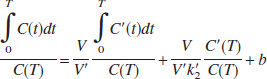
where C(t) and C′(t) are the regional or voxel timeradioactivity concentrations in the tissue and reference regions, respectively (kBq/mL), V and V′ are the corresponding total distribution volumes (mL/mL); k′2 (min−1) is the clearance rate constant from the reference region to plasma, and b is the intercept term, which becomes constant for T > t*. Eq. 1 allows estimation of three parameters, β1 = V/V′, β2 = V/(V′k′2), and β3 = b by multilinear regression analysis for T > t*. Note that Eq. 1 and all subsequent linear equations are applicable to both 1T and two-tissue (2T) compartment models. Assuming that the nondisplaceable distribution volumes in the tissue and reference regions are identical, BP (BP = V/V′ − 1) is calculated from the first regression coefficient as BP = (β1 − 1). For radioligands with 1T kinetics such as [11C]DASB (Ginovart et al., 2001), Eq. 1 is linear from T = 0, i.e., t* = 0, and b is equal to (−1/k2), where k2 (min−1) is the clearance rate constant from the tissue to plasma. For the 1T model, V = K1/k2 and V′ = K′1/k′2, where K1 and k′1 (mL/min−1 /mL−1) are the rate constants for transfer from plasma to the tissue and reference region, respectively, and R1 = K1/k′1, the relative radioligand delivery, can be calculated from the ratio of the second and third regression coefficients as R1 = −β2/β3.
Ordinary LS parameter estimation assumes that independent variables are noise-free. However, Eq. 1 contains a noisy term, C(T), on the right-hand side (independent variables). In addition, the structure of Eq. 1 makes noise in the dependent (lefthand side) and independent variables correlated. These factors produce biased estimates (Carson, 1993; Ichise et al., 2002; Slifstein and Laruelle, 2000). Following the strategy described previously to reduce noise-induced bias for linear estimation of V using tissue and blood data (Ichise et al., 2002), Eq. 1 can be rearranged to yield the following multilinear reference tissue model (MRTM):
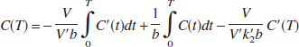
In Eq. 2, noisy C(T) is no longer present in the independent variables, although integral of C(t) is present. However, integrals of noisy data typically have much lower percent variation than the data themselves (Ichise et al., 2002). Additionally, the correlation of the noise in the dependent and independent variable is dramatically reduced in Eq. 2 compared with Eq. 1. Eq. 2 also allows estimation of three parameters, γ1 = −V/(V′b), γ2 = 1/b and γ3 = −V/(V′k′2b), assuming that the integrals of C(t) and C′(t), as well as C′(T), are noise-free. BP can then be calculated from the ratio of the two regression coefficients as BP = −(γ1/γ2 + 1). For the 1T model R1 = γ3 and k2 = −γ2.
Eq. 2 also allows estimation of k′2, which is given by k′2 = γ1/γ3. However, a different value of k′2 is estimated by Eq. 2 for each voxel, although there is only one reference region and therefore only one true value for k′2. By fixing k′2 to a value obtained with a preliminary analysis using Eq. 2, a two-parameter version of Eq. 2 (MRTM2) is obtained by rearrangement to yield
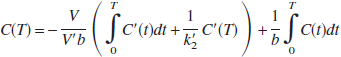
Eq. 3 can also be obtained by rearrangement of the graphical reference tissue model described by Logan et al. (1996). Eq. 3 estimates two parameters, γ1 = −V/(V′b) and γ2 = 1/b for T > t*, assuming that the integrals of C(t) and C′(t), as well as C′(T), are noise-free. BP is then calculated from the ratio of the two regression coefficients as BP = − (γ1/γ2 + 1). For the 1T model, R1 = γ1/k2 and k2 = −γ2. Because MRTM2 estimates fewer parameters, it is expected to be more stable than MRTM, particularly at high-noise levels of voxel-based parametric imaging. This strategy has been shown to be effective in reducing noise from the three-parameter simplified reference tissue model (SRTM) to the two-parameter model SRTM2 (Wu and Carson, 2002).
Simplified reference tissue models
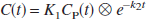
The operational equation for the SRTM (Lammertsma and Hume, 1996) is

where ⊗ is the convolution symbol. Note that Eq. 4 is derived from the 1T compartment model unlike the above linear equations that are applicable to both 1T and 2T compartment models. Eq. 4 allows NLS estimation of three parameters from the entire data set, R1, k′2, and k2. BP is calculated from the relationship, BP = R1(k′2/k2) − 1. In the two-parameter SRTM2 method (Wu and Carson, 2002), the value of k′2 is fixed so that Eq. 4 estimates two parameters, R1 and k2.
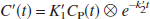
where CP(t) is the metabolite-corrected plasma concentration (kBq/mL). Eq. 5 allows NLS estimation of two parameters from the entire data set, K1 and k2. BP and R1 are calculated from the relationship, BP = (K1k′2/k′1k2) − 1 and R1 = K1/k′1, where k′1 and k′2 are estimated by 1TKA applied to the reference region time–activity curve (TAC), with the following equation:
Positron emission tomography studies
[11C]DASB PET studies were performed in eight normal control subjects (mean age, 21.8 ± 2.4 years; age range, 20–27 years). The study protocol was approved by the ethics and radiation safety committees of the National Institute of Radiological Sciences (Chiba, Japan), and written informed consent was obtained from each subject. [11C]DASB was synthesized as described previously (Wilson et al., 2000a,b). After a 10-minute transmission scan using a 68Ge-68Ga source, dynamic PET scans were acquired for 90 minutes (27 frames consisting of 4 × 1, 13 × 2, 5 × 4 and 5 × 8-minute frames) after bolus administration of 630 ± 51 MBq (specific activity, 70–196 GBq/μmol at the time of injection) of [11C]DASB on the ECAT 47 (CTI-Siemens, Knoxville, TN, U.S.A.) scanner in two-dimensional mode, which provides 47 slices with 3.38-mm center-to-center slice separation. To minimize head movement during each scan, head fixation devices (Fixster Instruments, Stockholm, Sweden) and thermoplastic attachments made to fit the individual subject were used. The PET data were reconstructed using a Hann filter with a cut-off frequency of 0.5 resulting in image full width at half maximum of 9.3 mm.
Arterial blood samples were taken 13 times during the initial 3 minutes after the tracer injection, then eight times during the next 17 minutes, and then once every 10 minutes until the end of the scan. Each blood sample was separated into plasma and blood cell fraction by centrifugation. For the plasma fractions at 3.5, 9, 19, 29, 39, 49, 59, 69, 79, and 89 minutes after injection, acetonitrile was added and the sample was centrifuged. The obtained supernatant was subjected to radio-HPLC analysis (column μBondapak C18; mobile phase, phosphoric acid [6 mmol/L]/CH3CN = 1:1; flow rate, 2.5 mL/min). The fraction of unchanged radioligand in plasma was fitted to a sum of two exponentials. A metabolite-corrected plasma curve was generated by the product of the plasma activity and metabolite fraction curves. The portion of the metabolite-corrected plasma curve beyond the initial peak was fit to a sum of two exponentials (three exponentials did not improve fitting). The resulting curve was used as the input function for estimation of 1T kinetic parameter values (see below). Plasma protein binding was not determined in the present study.
Simulation analysis
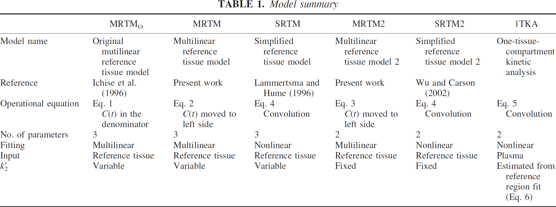
Table 1 lists the characteristics of the six models used for the simulation analysis and the analysis of human PET data. For the simulation, bias and variability of BP and R1 estimates by all six models due to statistical noise were evaluated with simulated [11C]DASB TACs at different noise levels. Gray matter regions with a range of BP (raphe, striatum, thalamus, and frontal cortex) were simulated. Even though BP measurement in white matter may not be of biological interest, simulations in white matter with very low BP were also performed because poor estimation characteristics there would contribute to artifacts in parametric images.
Model summary
In addition, the feasibility of obtaining a stable k′2 value to be used for MRTM2 and SRTM2 was evaluated by application of MRTM to ROI TACs. To this end, bias and variability of k′2 estimates by MRTM were calculated for simulated [11C]DASB TACs at different ROI noise levels. The variability of BP and R1 estimates from simulation were, when appropriate, compared with the respective theoretical variability, as predicted by the Cramer-Rao (C-R) lower bounds for the two-parameter and three-parameter models (Beck and Arnold, 1977; Wu and Carson, 2002).
To perform [11C]DASB TAC simulations, a metabolite-corrected plasma input function that had a typical clearance (175 L/h) was selected from a normal control study, and was scaled to a group mean injection dose of 630 MBq. TACs were simulated using the 1T parameter values (Table 2). Intravascular radioactivity was not included because its contribution would be minimal owing to the high K1 and V values. These parameter values were derived from the group mean k′1, K1, V′, and V values estimated by 1T KA for the respective regions (see below).
One-tissue-compartment kinetic parameter values used for simulating time-activity curves
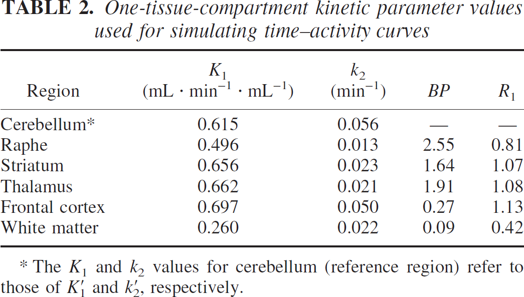
The K1 and k2 values for cerebellum (reference region) refer to those of k′1 and k′2, respectively.
Noise-free TACs were generated for 90 minutes (54 frames of 30-second to 4-minute duration with TAC values calculated at the midframe time). The sampling rates used in the simulations were twice the rates used in actual PET studies to minimize any bias introduced by the integral(s) on the right-hand side of the operational equations. Then, random amounts of normally distributed mean zero noise were added to the noise-free TAC with SD according to the following formula:
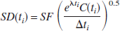
where SF is the scale factor that controls the level of noise; C(ti) is the noise-free simulated radioactivity; Δti is the scan duration (seconds); and λ is the radioisotope decay constant. This model is appropriate in the case of low or constant randoms fractions, constant scatter fraction, and relatively unchanging emission distribution over time. One thousand noisy TACs were generated for several values of SF so that TAC noise levels ranged from 5 to 30%. Percent TAC noise was calculated from the mean SD (Eq. 7) of the latter portion of the TAC (50 to 90 minutes). These noise levels would cover a range of TAC noise between that found in a small ROI to that of a voxel.
The noise-free reference tissue TAC for all reference tissue models and the true k′2 value of 0.056 min−1 for MRTM2 and SRTM2 were used in fitting noisy tissue TACs (see Discussion). Equal data weights were used for all methods (see Discussion). Because all TACs were simulated consistent with the 1T model, t* was set to 0 for MRTMO, MRTM, and MRTM2. The first time point was excluded from fitting, however, to minimize any bias introduced by the integral(s) on the right-hand sides of the operational equations. For SRTM, SRTM2, and 1TKA, the initial parameter values were chosen randomly from the range of 75 to 125% of the true parameter value. To calculate BP and R1 for 1TKA, the true values of k′1 and k′2 were used for consistency with the use of noise-free C′(t) in the reference tissue methods. Parameter estimates were considered outliers if BP or R1 values were less than zero or more than five times the true values, which should include nonconvergence cases. Bias was expressed as percent deviation of the sample mean from the true value and the variability was calculated as percent sample SD relative to the true value excluding outliers. Theoretical BP and R1 variability were calculated as percent C-R SD relative to the true value.
For MRTM2 and SRTM2, k′2 will be estimated by preliminary application of MRTM or SRTM to ROI TACs. To assess the magnitude of noise in this ROI-based k′2 estimation, 1,000 noisy tissue TACs were generated at noise levels ranging from 1 to 7%, which would cover a range of TAC noise found in large to small ROIs. k′2 was estimated by MRTM, with sample bias and sample variability of k′2 calculated as above. In addition, the effect of error in k′2 estimates on MRTM2 estimation of BP and R1 was evaluated by calculating the bias of BP and R1 estimates by fitting the original gray matter TACs using biased k′2 values (ranging from −6 to +6%). All simulation analyses were performed in MATLAB (The MathWorks, Natick, MA, U.S.A.), or pixel-wise kinetic modeling (PMOD) software (PMOD Group, Zurich, Switzerland).
Positron emission tomography study analysis
The original reconstructed PET data were corrected for subject motion by registering each frame to a summed image of all frames, and the summed PET image was coregistered to a T1-weighted magnetic resonance image (repetition time/echo time = 21/9.2 milliseconds), acquired on a 1.5-T Phillips Intera (Phillips Medical Systems, Best, The Netherlands), in both cases using a six-parameter mutual information registration technique (Jenkinson et al., 2002) in the image analysis software MEDx (Sensor Systems Inc., Sterling, Virginia, U.S.A). The summed PET image was then fused with the coregistered magnetic resonance image using an image fusion tool in PMOD. Several anatomical ROIs were manually defined on this fused image, and ROI TACs from the cerebellum (∼400 voxels, voxel size = 3.4 × 3.4 × 3.4 mm), raphe (∼40 voxels), striatum (∼110 voxels), thalamus (∼90 voxels), frontal cortex (∼400 voxels), and white matter (∼200 voxels) were obtained. These ROI TACs were fitted by 1TKA using individual metabolite-corrected plasma input functions. The mean 1TKA parameter values from five of eight subjects were used to generate noise-free TAC data, as described in the previous section regarding simulation analysis.
To compare voxel-wise BP and R1 estimates between the different reference tissue models as well as 1TKA, individualvoxel TACs were obtained from the raphe, striatum, and frontal cortex. MRTM2 and SRTM2 require a priori knowledge of value, which was provided by preliminary application of MRTM. To minimize the variability of estimation by MRTM (see the simulation results), a weighted (according to ROI size) mean value estimated from ROI TACs of raphe, striatum, and thalamus was used. To calculate BP and R1 for 1TKA, the values of k′2 and k′1 estimated by 1TKA for the cerebellar ROI were used. Parameter estimate outliers were arbitrarily defined as BP or R1 values less than zero or more than five times the same values used in the simulation analysis.
For comparison to simulations, percent ROI and voxel TAC noise was calculated based on deviations from 1TKA fitting for the latter portion of the TAC (50 to 90 minutes). ROI noise values [mean ± SD (range)] were 3.1 ± 1.0% (2.1–4.9%), 1.9 ± 0.5% (1.1–2.3%), 2.4 ± 0.6% (1.2–2.8%) and 2.6 ± 0.6% (1.8–3.1%) in the raphe, striatum, thalamus, and frontal cortex, respectively. Voxel noise values were 12 ± 4%, 11 ± 4%, 15 ± 5%, and 23 ± 8% in the raphe, striatum, frontal cortex, and white matter, respectively. If the actual scan data had been acquired with the doubled sampling rate, as used in the simulation, all these noise values would have increased by a factor of √2. Thus, for comparison to the simulations, the percent noise values in the actual PET data were multiplied by √2. Thus, ROI noise values of 3 to 7%, 2 to 3%, 2 to 4%, and 2 to 4% in the raphe, striatum, thalamus, and frontal cortex, respectively, and voxel noise values of 15% and 30% for gray and white matter, respectively, were chosen as typical noise levels in evaluating the simulation results.
Comparison of estimates between MRTM and 1TKA as well as comparison of voxel-based BP and R1 estimates between all methods were made by performing paired t-tests. Statistical significance was defined as P < 0.05.
Parametric images of BP and R1 were generated from the motion-corrected data sets (n = 8) by MRTMO (BP only), MRTM2, SRTM2, and SRTM, respectively. The SRTM and SRTM2 parametric imaging was performed based on the basis function method of Gunn et al. (1997) to improve processing speed. All parametric imaging was performed in PMOD installed on a PC workstation (Dell Computer Co., Austin, TX, U.S.A., 1.7 GHz Pentium IV/1 GB-RAM running Microsoft Windows 2000, Microsoft Co., Redmond WA, U.S.A). PMOD is platform-independent software programmed in Java environment (Mikolajczyk et al., 1998).
RESULTS
Simulation analysis
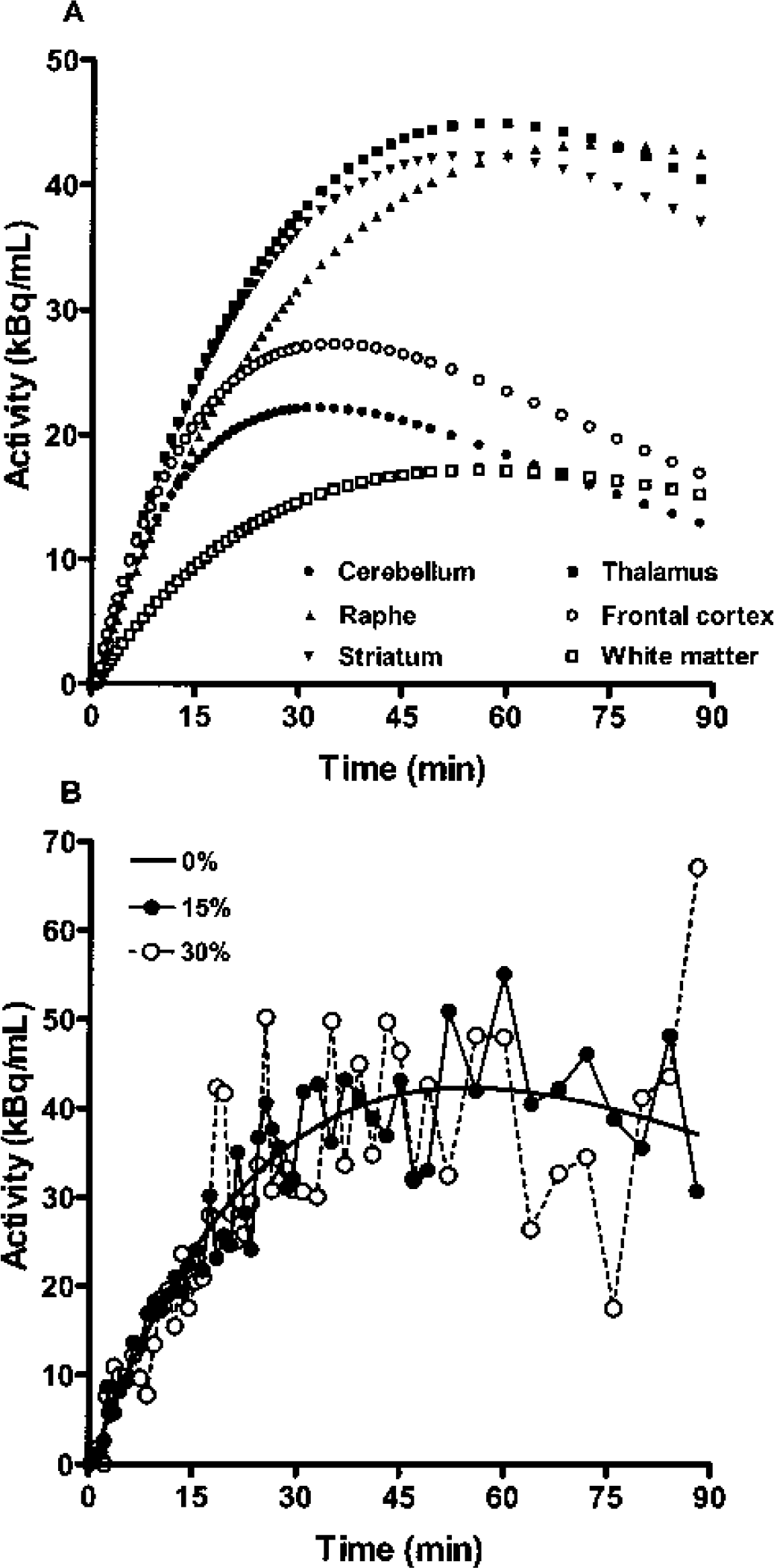
Simulated [11C]DASB noise-free time–activity curves (
Bias and variability of binding potential (BP) estimates by six different models for simulated [11C]DASB data at different noise levels
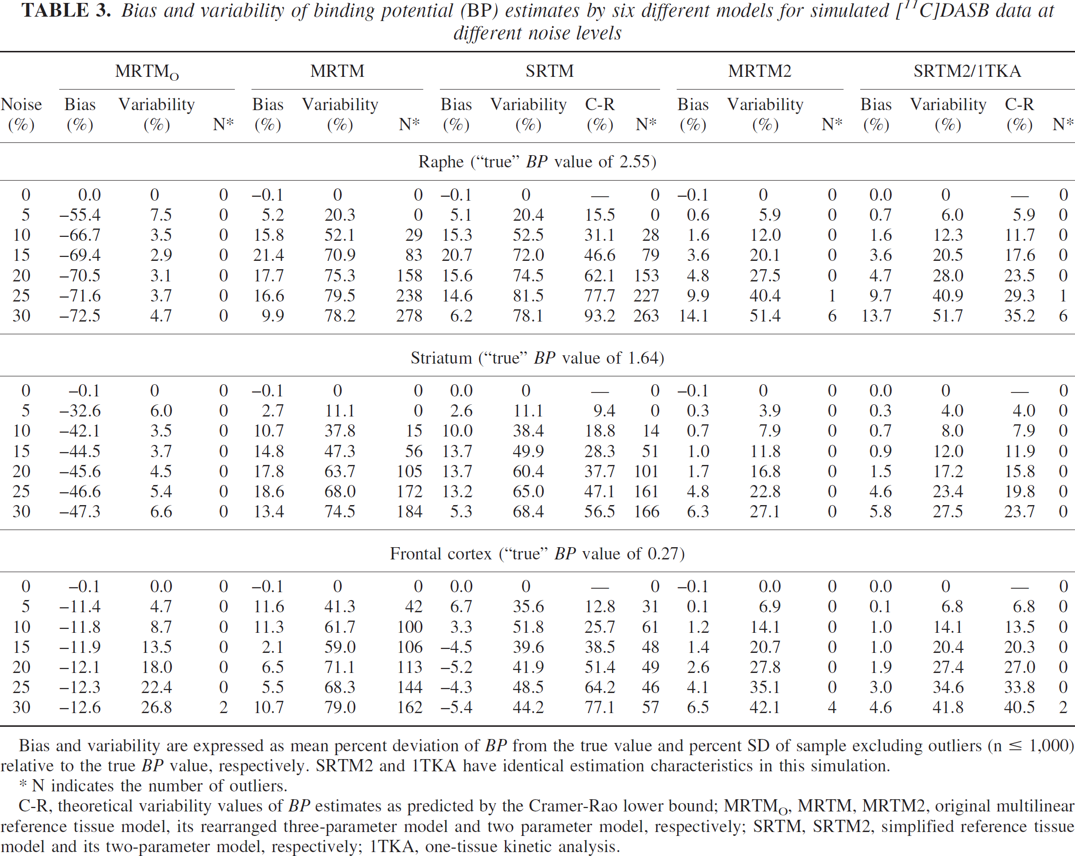
Bias and variability are expressed as mean percent deviation of BP from the true value and percent SD of sample excluding outliers (n ≤ 1,000) relative to the true BP value, respectively. SRTM2 and 1TKA have identical estimation characteristics in this simulation.
N indicates the number of outliers.
C-R, theoretical variability values of BP estimates as predicted by the Cramer-Rao lower bound; MRTMO, MRTM, MRTM2, original multilinear reference tissue model, its rearranged three-parameter model and two parameter model, respectively; SRTM, SRTM2, simplified reference tissue model and its two-parameter model, respectively; 1TKA, one-tissue kinetic analysis.
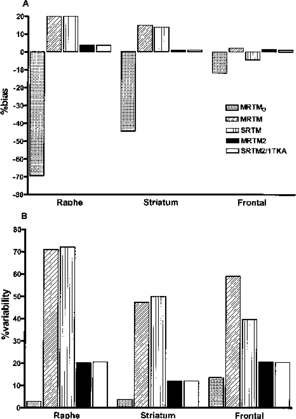
Bias (
MRTMO had the largest magnitude of bias (−12 to −70%, Fig. 2A), but the smallest variability (4–14%, Fig 2B), and no outliers except at the highest noise level (Table 3). MRTM and SRTM, had magnitudes of bias intermediate between MRTMO and MRTM2, SRTM2, or 1TKA (∼20%, Fig. 2A), the largest variability (40–70%, Fig. 2B), and large numbers of outliers up to 10% at 15% noise (Table 3). Unlike MRTM2, SRTM2, or 1TKA, the variability values for MRTM and SRTM showed a noticeable discrepancy from the C-R values, even at moderate noise levels (see Discussion). However, this discrepancy artifactually appeared to decrease with increasing number of outliers because the variability values were calculated excluding the outliers (Table 3). The bias and variability were similar for MRTM and SRTM in both the striatum and raphe. However, in the frontal cortex, MRTM had somewhat larger variability than SRTM, with more outliers at all noise levels (Table 3).
Thus, MRTM2, SRTM2 and 1TKA, given knowledge of k′2 all markedly reduced the magnitude of BP bias compared with MRTMO at the expense of somewhat increased variability. Furthermore, these methods considerably reduced BP bias in the high-BP regions and BP variability in all regions by a factor of two or three compared with MRTM or SRTM (Table 3).
For the white matter, however, BP estimation tended to be unstable for all methods, particularly for MRTMO, MRTM, and SRTM. For example, at the typical white matter noise level, BP estimates were all negative for MRTMO, whereas the mean ± SD (range) values of BP estimates over 1,000 runs for SRTM, MRTM2, and SRTM2/1TKA were −0.10 ± 6.48 (−168 to +93), 0.14 ± 0.22 (−0.29 to +2.08), and 0.13 ± 0.23 (−0.30 to +2.08), respectively. This instability of BP estimation in the white matter suggested that parametric images from these latter methods will contain some white matter voxels with inappropriately high positive BP values, due simply to statistical noise in the data. For example, histograms of BP estimates for MRTM2 and SRTM are shown in Fig. 3A, where 1% and 5% of voxels had BP values >1, respectively. Although the BP in the white matter is not generally of pathophysiologic interest, parametric images with noisy white matter voxels could be visually misleading.
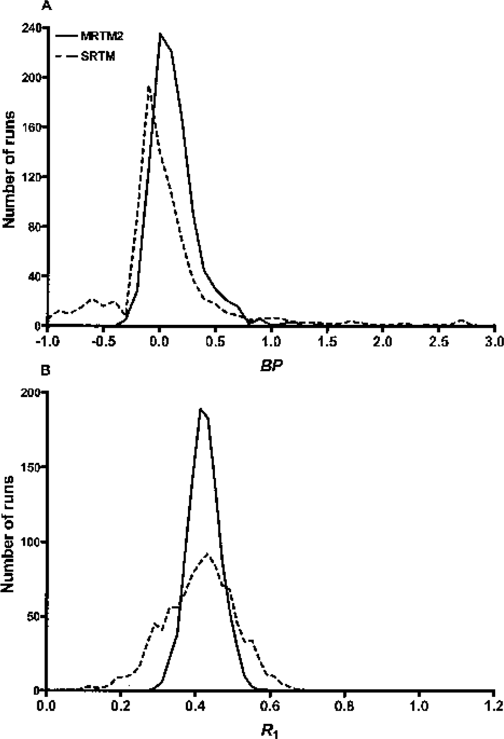
Histograms of estimated BP (
Bias and variability of relative delivery (R1) estimates by five different models for simulated [11C]DASB data at different noise levels
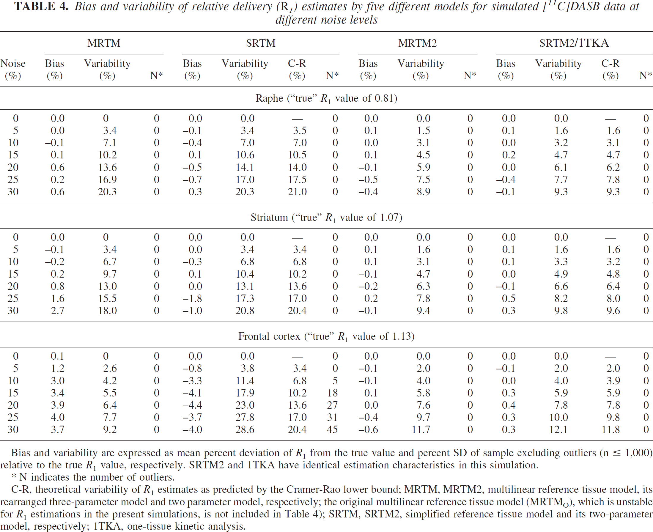
Bias and variability are expressed as mean percent deviation of R1 from the true value and percent SD of sample excluding outliers (n ≤ 1,000) relative to the true R1 value, respectively. SRTM2 and 1TKA have identical estimation characteristics in this simulation.
N indicates the number of outliers.
C-R, theoretical variability of R1 estimates as predicted by the Cramer-Rao lower bound; MRTM, MRTM2, multilinear reference tissue model, its rearranged three-parameter model and two parameter model, respectively; the original multilinear reference tissue model (MRTMO), which is unstable for R1 estimations in the present simulations, is not included in Table 4); SRTM, SRTM2, simplified reference tissue model and its two-parameter model, respectively; 1TKA, one-tissue kinetic analysis.
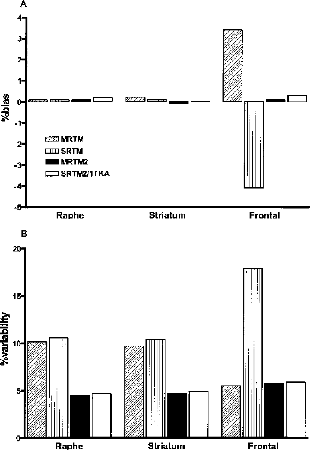
Bias (
Both MRTM and SRTM had slightly larger magnitudes of bias (up to 4%, Fig. 4A) and higher variability by a factor of two or three (Fig. 4B) than did MRTM2, SRTM2, or 1TKA, except that MRTM had variability in the frontal cortex comparable with that for MRTM2, SRTM2, or 1TKA (see Discussion). However, MRTMO R1 estimation (data not shown) was very unstable, with outliers exceeding 50% at 15% noise and beyond for all gray matter regions.
Finally, for the white matter, unlike BP estimates, R1 estimates by MRTM, SRTM, MRTM2, SRTM2 and 1TKA were stable with no outliers, as shown in the histogram for SRTM and MRTM2 in Fig. 3B.
Fig. 5 shows the correlation scatterplot between the MRTM2 parameter estimates γ1 and γ2 from the 1,000 simulated realizations in the three gray matter regions and white matter. For convenience of scale and interpretation, the parameters have been divided by k′2 so the x and y axes are R1 and k2/k′2, respectively. For a given region, the parameter estimates are correlated; this is reflected in the nonzero slope of the elliptical cloud of parameter estimates. For example, for voxels with lower than average R1, the estimated k2 also tended to be lower than the mean, resulting in increased values of BP. For white matter values, the spread of voxel noise produces a wide range of BP values with a long positive tail (Fig. 3A). The correlation plot in Fig. 5 suggested that appropriate thresholds using estimated R1 and BP values might lead to an algorithm that would eliminate the potentially misleading voxels in white matter with high BP values produced by noise. For example, the simplest approach would be to assign a BP value of zero to all voxels with R1 values below a certain cutoff value, which might result in cosmetically more satisfactory parametric BP images by removing these noise-induced high positive BP values within the white matter. The correlation scatter plot in Fig. 5 was virtually identical to that for SRTM2 (data not shown).
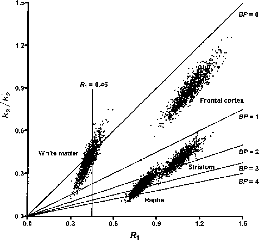
Relationship between R1 and BP estimates by MRTM2 for the three gray matter regions and white matter on a (k2/k′2) versus R1 plot, where k2 values were estimated from the second parameter in Eq. 3 as k2 = –γ2. Oblique straight lines indicate identical lines of different BP values (0, 1, 2, 3, and 4) calculated from the relationship k2/k′2 = R1/(BP + 1). Because positively higher BP values in the white matter have lover R1 values, assigning a BP value of zero to those voxels with low R1 values (e.g., R1 = 0.45 [vertical line]) would eliminate most of high positive BP values in the white matter. MRTM2, two-parameter multilinear reference tissue model; BP, binding potential; R1, relative delivery.
Bias and variability of k′2 estimates by three-parameter multilinear reference tissue model for simulated [11C]DASB region-of-interest data at differnt noise levels
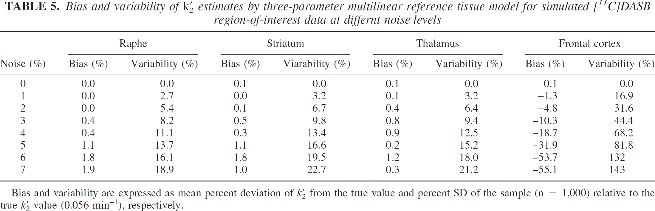
Bias and variability are expressed as mean percent deviation of k′2 from the true value and percent SD of the sample (n = 1,000) relative to the true k′2 value (0.056 min−1), respectively.
Error in the estimated value for each subject introduces bias in all the BP and R1 estimates for that subject. The magnitudes of MRTM2 bias in BP estimates due to biased k′2 estimates were 0.9, 0.4, and 0.1 times the bias of k′2 estimates for raphe, striatum, and frontal cortex, respectively (Fig. 6A). The corresponding magnitudes of bias in R1 estimates were smaller (i.e., 0.3, 0.2, and 0.04 times the bias of k′2 estimates; Fig. 6B). Thus, small biases k′2 estimates by MRTM for MRTM2 analysis would not result in any larger biases of BP or R1 estimates. The effects of biased k′2 on SRTM2 were identical to those of MRTM2 (data not shown).
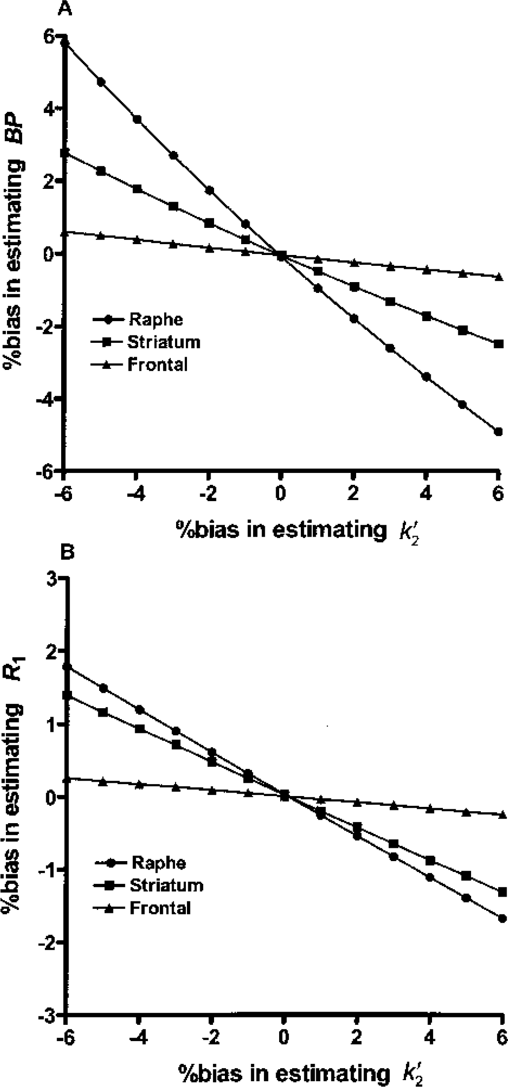
Sensitivity of BP (
Positron emission tomography study analysis
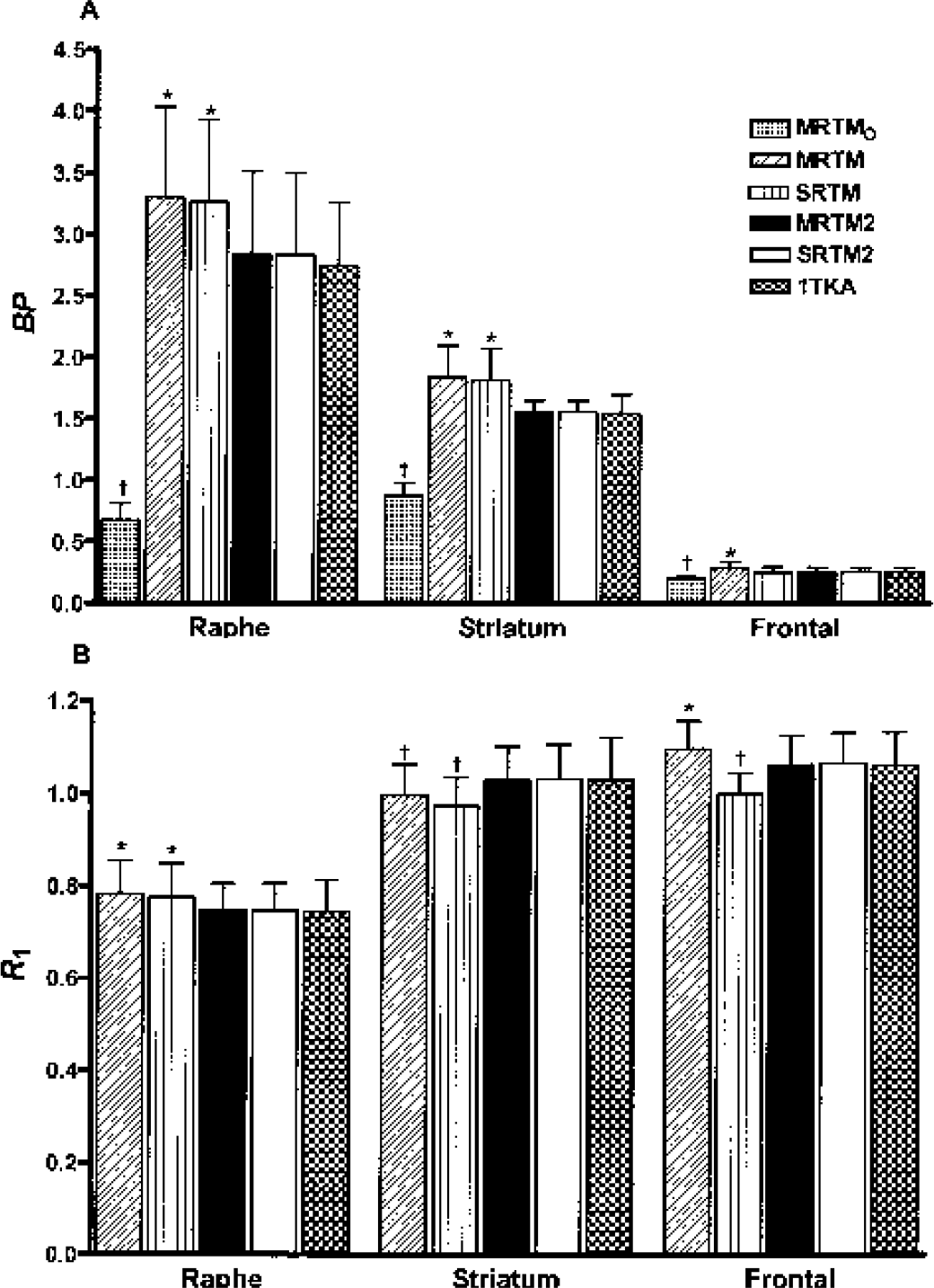
Mean regional BP (
The mean BP values estimated by MRTM were similar to those estimated by SRTM for raphe and striatum (Fig. 7A), with respective percent differences between the two models of 1 ± 3% and 2 ± 2%. However, the MRTM BP values for frontal cortex were somewhat higher (12%) than the corresponding SRTM BP values. The mean BP values estimated by MRTM or SRTM were higher (by ∼16% and ∼18% in the raphe and striatum, respectively) than those estimated by MRTM2 (Fig. 7A). These between-method BP differences were consistent with the simulations, where percent BP bias differences between MRTM and MRTM2 were ∼18% and ∼14% in the raphe and striatum, respectively; and the differences between MRTM and SRTM in the frontal cortex was ∼7% (Table 3).
The mean BP values estimated by MRTMO were strikingly lower by 76%, 44%, and 22% in the raphe, striatum, and frontal cortex, respectively, than those estimated by MRTM2 (Fig. 7A). These BP differences between MRTMO and MRTM2 were also consistent with the simulation results, where percent BP bias differences between the two models were ∼73%, ∼46%, and ∼13% in the raphe, striatum, and frontal cortex, respectively (Table 3).
Voxel BP outliers represented sizable percentages for both MRTM and SRTM (27%, 6%, and 15% of voxels in the raphe, striatum, and frontal cortex, respectively). However, there were no outliers for MRTMO, MRTM2, SRTM2, or 1TKA, as predicted by the simulations. The number of outliers for MRTM and SRTM was larger than that predicted by the simulations, particularly for raphe (Table 3). This increased outlier percentage for MRTM and SRTM was due to increased number of low (negative) BP values, where the low-to-high outlier ratios were approximately three times those in the simulations, and may be a result of partial volume effects inherent in the actual PET data.
As predicted by the simulations, the MRTM2 R1 values were effectively identical to the SRTM2 R1 values (Fig. 7B), with percent differences between the two models of 0.0 ± 0.1%, −0.3 ± 0.1%, and −0.3 ± 0.2% for raphe, striatum, and frontal cortex, respectively. As was the case for BP, the MRTM2 R1 values were similar to the 1TKA R1 values (Fig. 7B), with percent differences between the two models of 0.5 ± 3.0%, 0.0 ± 3.0%, and 0.1 ± 1.0% for raphe, striatum, and frontal cortex, respectively. The mean R1 values estimated by MRTM were similar within 2% to those estimated by SRTM for raphe and striatum. However, the MRTM R1 values for frontal cortex were somewhat higher (10%) than the corresponding SRTM R1 values. The mean R1 values estimated by MRTM or SRTM were higher (∼5% in the raphe) and lower (∼5% in the striatum) than those estimated by MRTM2 (Fig. 7B). These R1 differences between MRTM and SRTM were consistent with the simulations, where the respective percent R1 bias differences were <1% in both the raphe and striatum and ∼8% in the frontal cortex, respectively. However, these R1 differences between MRTM or SRTM and MRTM2 in the raphe and striatum were slightly larger compared with the simulations, where the corresponding percent R1 bias differences were <1% (Table 4). MRTMO was very unstable for R1 estimation with large percentages of outliers exceeding 50% (data not shown), as was the case in the simulations. There were no outliers of R1 estimates for the other models except for SRTM, where there were a small number of outliers (2%) in the frontal cortex but none in the raphe or striatum with the outlier percentage very consistent with the simulations (Table 4).
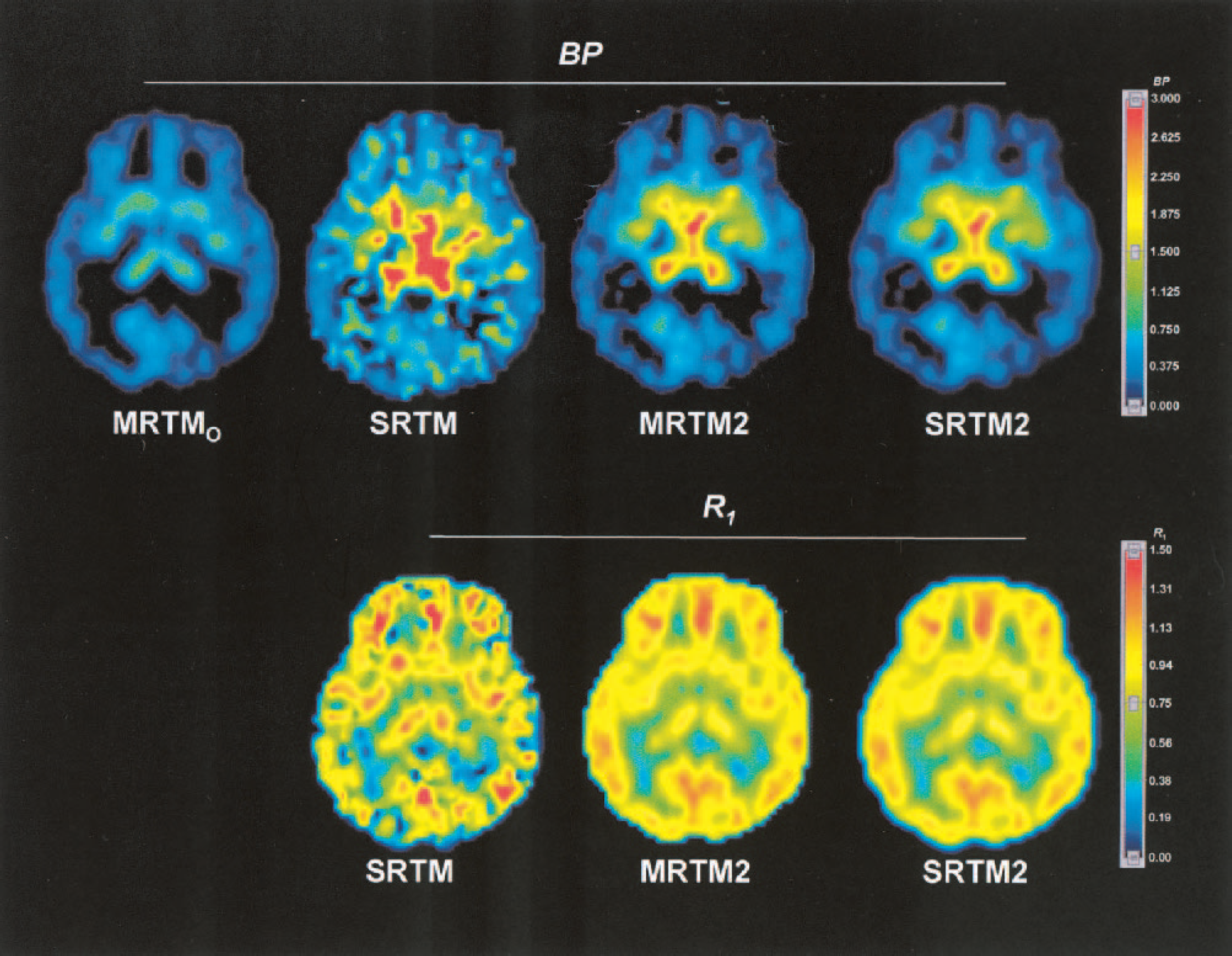
Parametric images of [11C]DASB BP (top row) estimated by MRTMO, SRTM, MRTM2, and SRTM2, and R1 (bottom row) estimated by SRTM, MRTM2, and SRTM2. BP, binding potential; R1, relative delivery; MRTMO and MRTM2, original multilinear reference tissue model and its rearranged two-parameter model, respectively; SRTM and SRTM2, simplified reference tissue model and its two-parameter model, respectively.
Fig. 9 shows examples of BP and R1 parametric images estimated by MRTM2 and the corresponding magnetic resonance images from the same subject. In the BP images, voxels with corresponding R1 values below 0.45 were set to 0. In this subject, all of these voxels belonged anatomically to the white matter region on the coregistered magnetic resonance scan (data not shown). This process improved the appearance of white matter regions in the BP image by removing the misleading noiseinduced high BP values. The BP images (left column) show that regionally BP values are high in the hypothalamus and raphe, moderately high in the thalamus and striatum, and low to very low in the amygdala and cerebral cortex, respectively. This regional BP pattern was consistent with the known regional distributions of SERT sites. The R1 images (middle column) show that R1 values are high to moderate in the cortex, striatum and thalamus; and relatively low in the hypothalamus, raphe and amygdala, respectively. This regional R1 pattern was consistent with human imaging studies of cerebral blood flow.
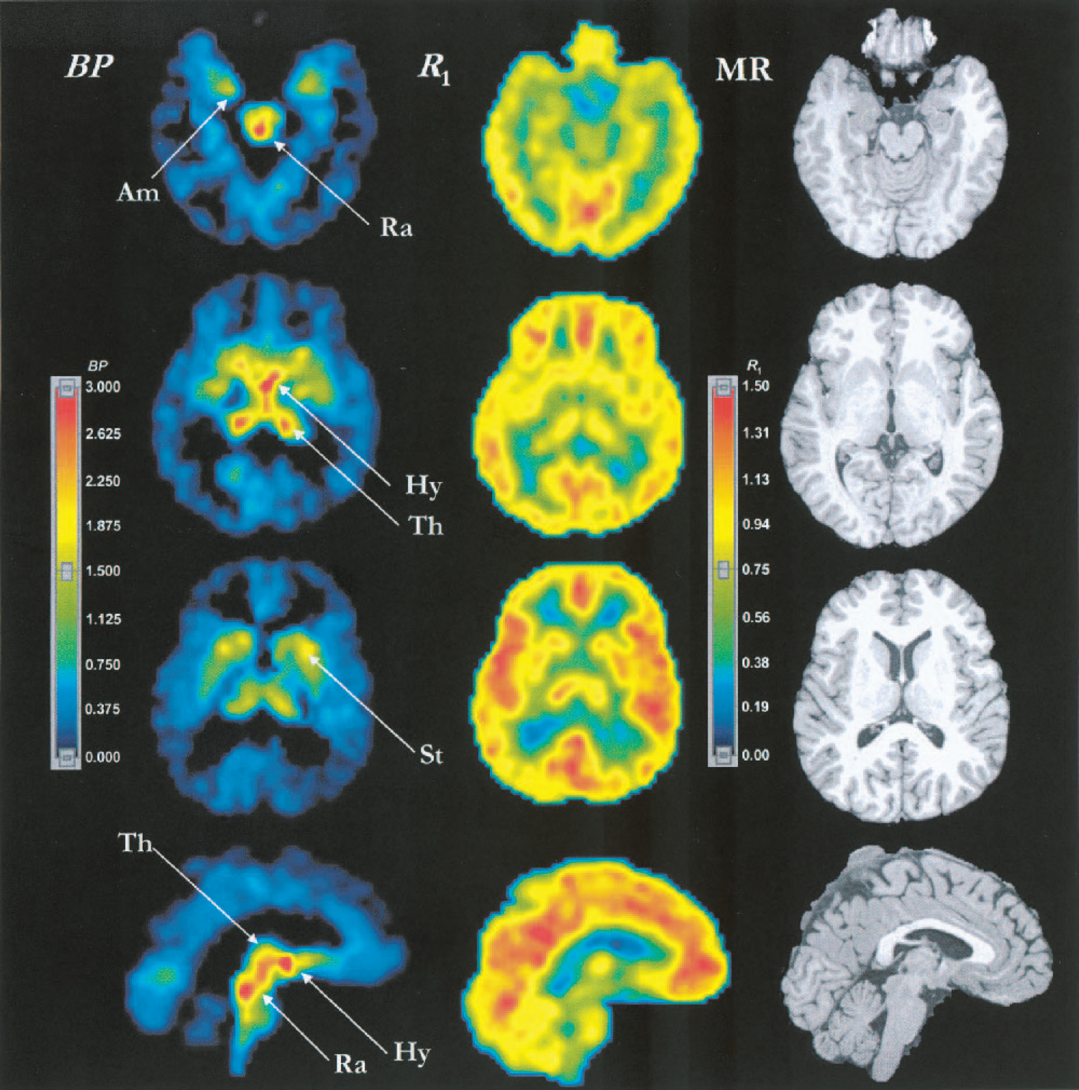
Parametric images of [11C]DASB BP (left column) and R1 (center column) estimated by MRTM2, and T1-weighted magnetic resonance images (right column). In the BP images, all voxels with corresponding R1 values below 0.45 were set to zero. The top three rows show transverse images and the bottom row shows sagittal images. The BP image in the second row corresponds to the MRTM2 BP image in Fig. 8. The color display ranges for BP and R1 images are 0 to 3.0 and 0 to 1.50, respectively. Am, amygdala; Hy, hypothalamus; Ra, raphe complex; St, striatum; Th, thalamus; BP, binding potential; R1, relative delivery; MRTM2, two-parameter multilinear reference tissue model.
The threshold R1 value of 0.45 removed 1,800 ± 400 voxels (∼70 mL) from the white matter and the resulting BP images were visually considered satisfactory in six of eight subjects. There were a few white matter voxels with noise-induced moderately high BP in one of the two remaining subjects. In this subject, raising the threshold value to 0.47 removed those misleading voxels. In another subject, the thresholding process produced several sharp edges around the gray matter structures with relatively low flow such as the raphe and hypothalamus, although there were no misleading high-BP voxels in the white matter. In this subject, lowering the R1 threshold value to 0.42 improved the white matter image appearance by removing the sharp edges without reintroducing any visually misleading high-BP voxels.
DISCUSSION
In the present study, we applied two strategies to the original multilinear reference tissue model, MRTMO, to improve parametric images of BP and R1 for human [11C]DASB PET data. First, rearrangement of the MRTMO operational equation removed a noisy tissue radioactivity term, C(T), from the independent variables, and this MRTM decreased the bias of BP estimation substantially, at the expense of considerably increased variability. The three-parameter linear method, MRTM, has similar parameter estimation characteristics to the three-parameter nonlinear method, SRTM (Lammertsma and Hume, 1996). Although this increased BP variability with MRTM over MRTMO did not allow stable BP estimations at the voxel level, MRTM did allow estimation of k′2 with little bias (<1%) and relatively small variability (<6%) from cerebellar and several tissue ROI data. Second, assuming that there is only one k′2 value for the reference region, the number of parameters to estimate was reduced from three in MRTM to two in MRTM2 by using a common value of k′2, in a manner analogous to that used in the nonlinear method SRTM2 (Wu and Carson, 2002). MRTM2 substantially decreased the bias and variability of BP and R1 estimations over the linear and nonlinear three-parameter estimation methods. Furthermore, the linearized approach allowed rapid generation (<15 seconds) of stable parametric images of BP in the gray matter and R1 in the whole brain.
We previously evaluated the effects of the first strategy used here for the estimation of the distribution volume with plasma input function data for two neuroreceptor radioligands, [18F]FCWAY and [11C]MDL 100,907 (Ichise et al, 2002). The resulting linear model (referred to as MA1 in that study) was also nearly identical to its nonlinear counterpart for V estimation at the voxel level. Like MRTM2, the operational equation for MA1 has only two parameters to estimate. However, for estimation of BP without blood data, an additional parameter appears in the operational equations for both linear and nonlinear reference tissue models, which causes parameter estimation to be less stable under certain circumstances. Therefore, the second strategy of determining a single value for the reference region clearance constant and reducing the number of parameter from three to two was applied for these reference tissue models.
SRTM2 has been developed by Wu and Carson (2002) and evaluated in comparison with SRTM for three radioligands, [18F]FCWAY (5-HT1A), [11C]flumazenil (benzodiazepine), and [11C]raclopride (dopamine D2), where the magnitude of improvement in parameter estimation by eliminating one parameter depended on the radioligand's kinetics. In that study, the largest impact of SRTM2 on BP estimation was found for [11C]flumazenil, particularly with a 30-minute scan duration, where BP variability was reduced from ∼10 to ∼5% and R1 variability was reduced by a comparable degree. SRTM2 had a similar pattern of impact for [11C]DASB in the present study, although the magnitude of BP noise reduction was even larger.
To understand this behavior, consider the characteristics of the 1T model. Information in the data pertaining to V or BP is obtained at later times, as each tissue region approaches transient equilibrium with the plasma. Mathematically, this follows the function [1 – exp(−k2t)] as it approaches the value 1. In this framework, ignoring differences in the input function, a 90-minute [11C]DASB scan has kinetically similar characteristics to a 30-minute [11C]flumazenil scan, by having a similar value of k2t at the end of the study. For [11C]DASB in the raphe, k2 = 0.013 min−1, t = 90 minutes, and k2t = 1.17, whereas for [11C]flumazenil in the occipital cortex, k2 = 0.040 min−1, t = 30 minutes, and k2t = 1.20. This comparison also clarifies why, for [11C]DASB, the variability of voxel BP estimates in the raphe (20%) by SRTM2 or MRTM2 was larger than that in the striatum (12%), where k2t = 2.04 (Fig. 1A). This explanation is consistent with the corresponding larger C-R variability values for raphe of 18% compared with 12% for striatum (Table 3). Thus, a [11C]DASB scanning duration of more than 90 minutes may further improve parameter estimation at the voxel level for regions with very high BP such as the raphe, although Ginovart et al. (2001) showed that a 90-minute study is probably adequate for ROI-based [11C]DASB analyses.
We used the Cramer-Rao lower bound as a prediction of the minimum possible variance that can be achieved by unbiased estimators. Minimum-variance unbiased estimators are generally desirable, and least-squares estimators usually have these characteristics for linear models (i.e., when the model equations are linear with respect to all the parameters). For nonlinear models, these characteristics are achieved asymptotically (i.e., for low noise). Thus, for nonlinear models, as noise increases, the estimators become biased and the variance diverges from the C-R bound. This can be seen in Table 3 by comparing the BP variability values for SRTM and SRTM with their respective C-R values with increasing noise. Note that divergence of the sample variance from the C-R variance occurs at different noise levels depending on the model and the parameter values. For example, at 15% noise for striatum BP (Table 3), sample variability for SRTM is dramatically higher than the C-R bound, whereas the SRTM2 sample variability agrees with its theoretical prediction. Also, the R1 parameter, which appears linearly in the model (Eq. 4), shows an excellent match between sample and C-R variability up to the highest noise levels for SRTM and SRTM2 (Table 4).
From a statistical point of view, the multilinear estimators MRTMO, MRTM, and MRTM2 are not minimum-variance unbiased estimators, because of the use of noisy data C(T) in the independent variables (Eqs. 1–3). However, as shown in the Results, the magnitude of bias and variance depends considerably on the structure of the model and the parameter values. MRTMO produces estimates with large bias and variability smaller than the C-R bound. MRTM generally matches the bias and variance of its nonlinear version, SRTM. However, an interesting estimation condition occurs for MRTM in the frontal cortex. Because of the small BP value, there is little difference between the frontal cortex and cerebellum TACs (Fig. 1), and the three-parameter estimation (Eqs. 2 and 4) is unstable. This instability produces different results between the nonlinear SRTM and the linear MRTM. This can be seen in the higher MRTM BP variability compensated by lower MRTM R1 variability. This effect is due to the high correlation between the first and second independent variables in Eq. 2 for the frontal cortex. Alternatively, MRTM2, while technically not a minimum-variance unbiased estimator, provides identical estimation characteristics for all regions to the corresponding NLS method SRTM2 for [11C]DASB (Tables 3 and 4). It is likely that similar statistical results can be obtained with MRTM2 for other ligands that follow 1T kinetics.
In the simulations, we used a noise-free reference tissue TAC for the reference tissue methods and a noise-free plasma input function for 1TKA. Noise in a reference TAC or plasma input curve would have a global effect on the estimates (i.e., all voxel or ROI estimates for that subject would be affected in a common way). Therefore, this noise would not be reflected in the statistical noise of the image, as estimated in the simulation (Tables 3 and 4, Figs. 2 and 4). Rather, this source of noise would increase intersubject variation and degrade the reproducibility of parameter measurements. In our PET data, the intersubject variability of 1TKA and MRTM2 results were comparable, suggesting that these noise sources are either small or of comparable magnitude.
The simulation results for 1TKA were numerically identical to those of SRTM2 to three significant digits because (1) the operational equation SRTM2 (Eq. 4) is simply a different parameterization of Eq. 5 for 1TKA; (2) for the SRTM2 simulations, the true value of k′2 was used; and (3) for the 1TKA simulations, the true values of k′1 and k′2 were used for calculation of BP and R1. The subtle differences between the two methods were due to slight numerical integration errors of either the reference tissue TAC or plasma TACs. However, for the human PET data, 1TKA and SRTM2 were no longer identical because of the effects of input function measurement errors on 1TKA and differences in k′2 determination between the two methods.
There are a number of technical issues involved in implementing these methods. Both MRTM2 and SRTM2 require accurate a priori estimation of k′2. The simulation results indicated that k′2 estimation by MRTM using a single-tissue ROI such as the striatum has moderate variability (10%) of k′2 estimates, although the bias is very small (<1%). This noise in an individual's k′2 estimate would translate into a bias in all BP and R1 values for that subject (Fig. 6). To reduce this noise, we estimated k′2 values for several tissue ROIs and used a weighted mean of these values for MRTM2 and SRTM2. This strategy reduced the effective variability of k′2 estimates to less than 6%. Alternatively, Wu and Carson (2002) used the median value of estimated by SRTM for all brain voxels with moderate to high BP. The use of the median was necessary in their case to avoid bias induced by the noise of each pixel TAC. The median was not required here, using an ROI-based approach for k′2 estimation. Use of the nonlinear SRTM for this purpose can be computationally time consuming, and MRTM could be used instead to improve the processing speed. In any case, the optimal approach for MRTM or SRTM k′2 estimation should be carefully evaluated for each neuroreceptor radioligand of interest.
For the white matter with very low BP, voxel-wise BP estimation by MRTM2 was somewhat unstable, although MRTM2 reduced white matter noise considerably compared with SRTM (Figs. 5 and 8). To improve the appearance of the white matter in the MRTM2 BP image, we used a simple threshold based on a fixed R1 value. The disadvantage of this approach is that an appropriate threshold R1 value may differ between subjects (see Results). By increasing the threshold R1 value, sharp edges appeared around gray matter structures with relatively low blood flow, such as the raphe and hypothalamus, because R1 values in the neighboring voxels are below the threshold owing to the partial volume effect. An alternative approach to setting BP to 0 for R1 values below a specific cutoff would be to add a constraint to the least-squares fitting, so that parameter estimates are limited to a bounded region in parameter space (Fig. 5). This can be implemented with a two-step procedure, whereby voxels falling outside the permitted space can be refit to find the LS parameter values that fall on the boundary of the permitted space.
To minimize any bias introduced by the integral(s) on the right-hand side of the operational equations (Eqs. 1–4), the sampling rates used in the simulations were twice the rates used in the actual PET data. In addition, the first time point was excluded from fitting. This resulted in bias of no more than 0.1% for all methods in BP, R1, and k′2 estimations with noise-free data (Tables 2–4). Reduction of the sampling rates to those of actual PET data (27 frames) increased the magnitude of bias to approximately 0.3% for all models. Thus, for [11C]DASB, a very high sampling rate is not necessary to avoid integration-induced bias.
In this study, parameter estimation was performed without data weighting. However, MRTM2 (Eq. 3), SRTM2 (Eq. 4), and 1TKA (Eq. 5) can all be applied using weighted least squares estimation to account for noise-level differences in C(T) (Carson, 1986). Using the ideal weights, 1/Var[C(T)], for the current simulated data, weighted least squares improved the bias and variability of BP and R1 estimations by MRTM2 and SRTM2 slightly across all noise levels. For example, the BP bias and variability in the raphe by SRTM2 at 15% noise were 2.5% and 16.0% with weighted least squares, and 3.6% and 20.5% unweighted, respectively. Thus, weighted least squares improves parameter estimation when there is a considerable scan-to-scan variation in noise, as was the case for our 90-minute [11C]DASB PET study with the short half-life of 11C (20.4 minutes) (Fig. 1B).
The two-parameter linear (MRTM2) and nonlinear (SRTM2) models were effectively identical for voxel-wise parameter estimation for these [11C]DASB data. The major advantage of MRTM2 over SRTM2 is the parametric image computation speed, where SRTM2 is more computationally expensive. MRTM2 has another potential advantage over SRTM or SRTM2 in that the linearized models can be applied without assumption of a specific compartment configuration (Logan et al., 1990), as opposed to SRTM or SRTM2 that assume a 1T model for both the reference and tissue regions (Lammertsma et al., 1996). Violations of these compartment model assumptions with SRTM and SRTM2 have been shown to cause biased estimates irrespective of statistical noise in the PET data (Slifstein et al., 2000; Wu and Carson, 2002). However, there are a few issues to be addressed in applying MRTM2 for data that is inconsistent with the 1T model assumptions. First, the parameter R1 can no longer be estimated accurately, because b in Eq. 3 is not equal to (−1/k2), but is instead a function of the rate constants k2, k3, and k4 of the 2T model (Ichise et al., 2002; Logan et al., 1990). Second, the fit must be restricted to the “linear” portion of the data (i.e., t > t*, and t* must be defined). Because the operational equation is asymptotically linear, identification of t* can be problematic, particularly in the presence of noise in the data (Ichise et al., 2002). Another problem is that t* may be quite late for 2T radioligands with slow kinetics, resulting in increased statistical noise in the parameter estimates.
Finally, the voxel BP and R1 values estimated by MRTM2 or SRTM2 without blood data in our eight [11C]DASB PET studies were very similar to those estimated by 1T KA with plasma input function data. Ginovart et al. (2001) have also shown in their ROI-based data analysis that ROI BP values estimated by SRTM correlate well with those by 1TKA for their five human [11C]DASB PET studies. In addition, these investigators have noted that the regional distribution of BP appears to correlate well with the known distribution of the SERT densities in human brain (Ginovart et al., 2001; Houle et al., 2000). The BP parametric images (Figs. 8 and 9) also support these findings. Compared with ROI-based parameter estimations, however, parametric images will allow voxel-based statistical analysis of SERT binding sites throughout the brain, including small structures such as the raphe, hippocampus, and amygdala.
CONCLUSIONS
The two-parameter linearized reference tissue model, MRTM2, which incorporates two strategies to improve parameter estimation at the voxel noise level, allows rapid generation of stable parametric images of binding potential and relative delivery for [11C]DASB PET data. The noise reductions are effectively identical to those of the two-parameter nonlinear reference tissue model, but the computational time is dramatically shortened. This noninvasive MRTM2 should be a useful data analysis tool for [11C]DASB PET studies of the serotonin transporter in human brain.
Footnotes
Acknowledgments:
The authors thank Dr. Cyrill Burger for implementing the multilinear reference models in PMOD, Jude Gustafson, M.A., for editing assistance, and the entire PET Department Staff for technical assistance at the National Institute of Radiological Sciences, Chiba, Japan.