Sage Journals: Discover world-class research

Abstract

In an attempt to improve neuroreceptor distribution volume (V) estimates, the authors evaluated three alternative linear methods to Logan graphical analysis (GA): GA using total least squares (TLS), and two multilinear analyses, MA1 and MA2, based on mathematical rearrangement of GA equation and two-tissue compartments, respectively, using simulated and actual PET data of two receptor tracers, [¹⁸F]FCWAY and [¹¹C]MDL 100,907. For simulations, all three methods decreased the noise-induced GA bias (up to 30%) at the expense of increased variability. The bias reduction was most pronounced for MA1, moderate to large for MA2, and modest to moderate for TLS. In addition, GA, TLS, and MA1, methods that used only a portion of the data (T > t*, chosen by an automatic process), showed a small V underestimation for [¹¹C]MDL 100,907 with its slow kinetics, due to selection of t* before the true point of linearity. These noniterative methods are computationally simple, allowing efficient pixelwise parameter estimation. For tracers with kinetics that permit t* to be accurately identified within the study duration, MA1 appears to be the best. For tracers with slow kinetics and low to moderate noise, however, MA2 may provide the lowest bias while maintaining computational ease for pixelwise parameter estimation.

Keywords

Positron emission tomography Graphical analysis Linear regression analysis Parameter estimation Noise-induced bias

Dynamic positron emission tomography (PET) data allow estimation of physiologic parameters, for example, by applying compartmental kinetic models and nonlinear least squares (NLS) estimation methods. Nonlinear least squares methods have the theoretical advantage of providing minimum variance parameter estimates with little or no bias. The NLS methods can be computationally expensive, however, particularly for the purpose of pixelwise parameter estimation from three-dimensional PET data (Motulsky and Ransnas, 1987). Alternatively, linear least squares (LLS) methods are computationally more robust; that is, by not requiring an iterative search in parameter space, they avoid the convergence problems that may arise with the NLS methods. However, LLS estimation requires some form of linearization of the standard compartment model equations (Blomqvist, 1984; Gjedde, 1982; Logan et al., 1990; Patlak et al., 1983), because the standard solutions to these equations are nonlinear with respect to some of the parameters. Of the linear methods, the graphical methods developed by Patlak et al. (1983) and Logan et al. (1990) and their extensions permit the estimation of a subset of parameters and have been used extensively because of their computational simplicity.

For reversibly binding neuroreceptor tracers, the graphical analysis (GA) plot of Logan et al. (1990) allows estimation of the total distribution volume (V) from the slope of the graph (i.e., the LLS regression coefficient). The advantages of GA include its simplicity and model independence; that is, no knowledge is required of the compartmental configuration of the underlying data. Operationally, since linearity is not achieved from the beginning of the data set, a period for linear fitting (T > t*) must be determined. The value of t* depends upon the regional tracer kinetics. One drawback of GA is that in the presence of statistical noise in the PET data, GA underestimates V (Carson, 1993; Slifstein and Laruelle, 2000). To reduce the bias in GA, Logan et al. (2001) applied the iterative method developed by Feng et al., (1993, 1996), called generalized linear least squares (GLLS), as a technique to smooth the time-activity curves (TACs) and demonstrated that this strategy can effectively reduce the noise-induced bias. For the two-tissue (2T) compartment model, the GLLS method is applied to the data in two parts to generate smooth TACs (Logan et al., 2001).

The purpose of the present study was to evaluate alternative noniterative linear methods that are directly applicable to the 2T model as strategies to improve V estimation, particularly to reduce noise-induced bias. In ordinary least squares (OLS) estimation, the independent variables are assumed to be noise-free. However, the GA equation contains a noisy tissue radioactivity term, C(T), in the independent variable, which will contribute to a biased least-squares estimation. Therefore, an alternative approach is total least squares (TLS) estimation that accounts for noise in the independent as well as the dependent variables (Van Huffel and Vandewalle, 1991). Total least squares estimation has been recently proposed for GA by Varga and Szabo (2002), who referred to it as the “perpendicular linear regression model.” Another approach was to rearrange the GA equation in multilinear form to remove C(T) as an independent variable, although the integral of C(t) remains. This approach has been shown to be effective in reducing the noise-induced bias for the one-tissue (1T) compartment model (Carson, 1993). Finally, another multilinear equation with only integrals of C(t) in the independent variables was derived from the 2T model. This equation can be applied to the full data set, unlike GA or its multilinear form, which is applicable only beyond a certain time t*. In the present study, these linear methods and the NLS method were tested for noise-induced bias by data simulations and actual PET data of the 5-HT_1A tracer [¹⁸F]FCWAY (Carson et al., 2000a) and the 5-HT_2A tracer [¹¹C]MDL 100,907 (Watabe et al., 2000). These tracers were chosen because their kinetics require the use of at least a 2T compartment configuration for accurate data fitting.

MATERIALS AND METHODS

Theory

Total least squares

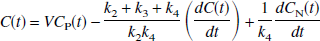
The operational equation for GA (Logan et al., 1990) is given by the following equation:

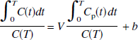
\frac{\int_{0}^{T} C (t) d t}{C (T)} = \frac{V \int_{0}^{T} C_{p} (t) d t}{C (T)} + b

(1)

where C(t) is the regional or pixel radioactivity concentration (kBq/mL) at time t, C_P(t) is the metabolite corrected plasma tracer concentration (kBq/mL) at time t, the slope (V) is the total distribution volume (mL/mL), and b is the intercept, which becomes constant for T > t*. For the 2T model, V is (K₁/k₂)(1 + k₃/k₄), where K₁ (mL·min⁻¹·mL⁻¹) is the rate constant for transfer from plasma to the nondisplaceable (free plus nonspecifically bound) compartment C_N, k₂ (min⁻¹) is the rate constant for transfer from C_N to plasma, k₃ (min⁻¹) is the rate constant for transfer from C_N to the specifically bound compartment C_S, and k₄ (min⁻¹) is the rate constant for transfer from C_S to C_N.

The OLS estimation assumes that independent variables are noise-free and that noise in the dependent variable is random with mean zero (Carson, 1986). However, Eq. 1 contains the noisy term C(T) in the independent variable, and the dependent and independent variables have correlated noise. Both of these conditions will contribute to a biased OLS estimation of V with Eq. 1. For OLS estimation, consider the case of the simplest example, where the model equation is given by y = βt, the parameter β, or the regression coefficient can be estimated by minimizing the cost function Q(β), which is the sum of squared differences between the observed values (n observations) of the dependent variable y_i and the fitted line; that is,

Q (β) = \sum_{i = 1}^{n} {(y_{i} - β t_{i})}^{2}

where the independent variable t_i is assumed noise-free (Carson, 1986). As an alternative, TLS minimizes the sum of squared “distances” of the observed points from the fitted line; that is,

Q (β) = \sum_{i = 1}^{n} {(y_{i} - β t_{i})}^{2} / (1 + β^{2})

is minimized. In the TLS formulation, both the dependent variable y_i and the independent variable t_i can contain independently distributed random errors with zero mean and equal variance (Van Huffel and Vandewalle, 1991). Thus, TLS may be useful for reducing the biased estimation because of the noisy term C(T) in the independent variable. However, the correlated noise in the dependent and independent variables in Eq. 1 can also be problematic for TLS since it assumes that the noise is uncorrelated (Van Huffel and Vandewalle, 1991). Because Eq. 1 contains the constant term b, one of the independent variable is noise-free. Thus, implementation of TLS minimization for Eq. 1 corresponds to the mixed OLS and TLS solution as described by Van Huffel and Vandewalle (1991).

Multilinear analysis 1

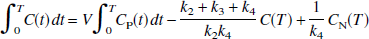
Alternatively, Eq. 1 can be rearranged to yield the following equation:

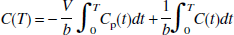
C (T) = - \frac{V}{b} \int_{0}^{T} C_{p} (t) d t + \frac{1}{b} \int_{0}^{T} C (t) d t

(2)

The OLS method is likely to be more appropriate for Eq. 2 than Eq. 1 because only the integral of C(t) appears as a potential noise source in the independent variables. Note that integrals of noisy data typically have much lower percent variation than the data themselves, particularly when only the later data (T > t*) are included in the linear fit. Also, the correlation of the noise in the dependent and independent variable is dramatically reduced in Eq. 2 compared to Eq. 1. Equation 2 is similar to the equation tested for the 1T model by Carson (1993). We propose use of Eq. 2 to estimate two parameters, β₁ = -V/b and β₂ = 1/b by multilinear regression analysis for T > t*, assuming that the integrals of the plasma and tissue data are noise-free. V then is calculated from the ratio of the two regression coefficients, −β/β₂. Note that both Eqs. 1 and 2 are asymptotically linear for T > t*; i.e., these equations are never identically linear and the instantaneous slope of these equations is always less than but approaching V (Logan et al., 1990; Slifstein and Laruelle, 2000). Therefore, if values of C for T < t* are included in the calculation, the LLS estimation with Eq. 1 or 2 would underestimate V, regardless of statistical noise.

Multilinear analysis 2

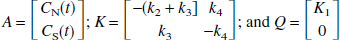
A multilinear equation valid for T > 0 with C(T) appearing only as integrals in the independent variables can be derived from the 2T model. This equation is a four-parameter version of the linear equation developed for three parameters (K₁, k₂, and k₃) by Blomqvist (1984), as described by Evans (1987). The differential equation describing the 2T model using the notation of Patlak et al. (1983) and Logan et al. (1990) is given by the following equation:

\frac{d A}{d t} = K A + Q C_{p} (t)

(3)

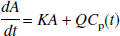
where

A = [\begin{array}{l} C_{N} (t) \\ C_{S} (t) \end{array}]; K = [\begin{array}{l} - (k_{2} + k_{3} & k_{4} \\ k_{3} & - k_{4} \end{array}]; and Q = [\begin{array}{l} K_{1} \\ 0 \end{array}]

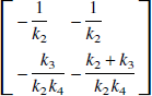
Eq. 3 can be rearranged to yield

A = - K^{- 1} Q C_{p} (t) + K^{- 1} \frac{d A}{d t}

(4)

where K⁻¹ is given by

\begin{array}{l} - \frac{1}{k_{2}} & - \frac{1}{k_{2}} \\ - \frac{k_{3}}{k_{2} k_{4}} & - \frac{k_{2} + k_{3}}{k_{2} k_{4}} \end{array}

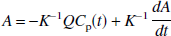
Equation 4 is equivalent to the following set of differential equations:

\begin{array}{l} C_{N} (t) & V_{N} C_{P} (t) - \frac{1}{k_{2}} \frac{d C_{N} (t)}{d t} - \frac{1}{k_{2}} \frac{d C_{S} (t)}{d t} \\ V_{N} C_{P} (t) - \frac{1}{k_{2}} \frac{d [C_{N} (t) + C_{S} (t)]}{d t} \end{array}

(5)

\begin{array}{l} C_{S} (t) & V_{S} C_{P} (t) - \frac{k_{3}}{k_{2} k_{4}} \frac{d C_{N} (t)}{d t} - \frac{k_{2} + k_{3}}{k_{2} k_{4}} \frac{d C_{S} (t)}{d t} \\ V_{S} C_{P} (t) - \frac{k_{2} + k_{3}}{k_{2} k_{4}} \frac{d [C_{N} (t) + C_{S} (t)]}{d t} + \frac{1}{k_{4}} \frac{d C_{N} (t)}{d t} \end{array}

(6)

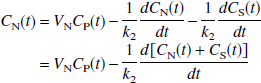
where V_N (mL/mL), given by (K₁/k₂), is the distribution volume of the nondisplaceable compartment (C_N), and V_S (mL/mL), given by K₁k₃/(k₂k₄), is the distribution volume of the specifically bound compartment (C_S). Addition of Eqs. 5 and 6, noting that V = V_N + V_S, yields

C (t) = V C_{P} (t) - \frac{k_{2} + k_{3} + k_{4}}{k_{2} k_{4}} + \frac{1}{k_{4}} \frac{d C_{N} (t)}{d t}

(7)

Note that under the condition of equilibrium (all derivatives = 0), Eq. 7 reduces to C(t) = V C_p(t), the definition of the total volume of distribution. Integration of Eq. 7 yields

\int_{0}^{T} C (t) d t = V \int_{0}^{T} C_{P} (t) d t - \frac{k_{2} + k_{3} + k_{4}}{k_{2} + k_{4}} C (T) + \frac{1}{k_{4}} C_{N} (T)

(8)

Insertion of Eq. 5 into Eq. 8 to eliminate C_N (t) and performing a second integration to eliminate the derivative, followed by rearrangement, yields

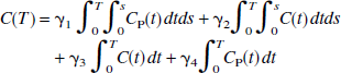
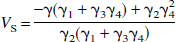
\begin{array}{l} C (T) = & γ_{1} \int_{0}^{T} \int_{0}^{s} C_{P} (t) d t d s + γ_{2} \int_{0}^{R} \int_{0}^{s} C (t) d t d s \\ + γ_{3} \int_{0}^{T} C (t) d t + γ_{4} \int_{0}^{T} C_{P} (t) d t \end{array}

(9)

where γ₁ = k₂k₄V, γ₂ = -k₂k₄, γ₃ = -(k₂ + k₃ + k₄), and γ₄ = K₁. If we assume that there are no radiolabeled metabolites in plasma, the contribution of vascular radioactivity to C can also be included into the derivation of Eq. 9 (Appendix). Note that Eq. 9 has C(t) in the independent variables only as single and double integrals. Eq. 9 allows LLS estimation of V by multilinear regression analysis utilizing the entire data set (T > 0), assuming that C_P and the integrals of the plasma and tissue data are noise-free. V is calculated as the ratio of the first two partial regression coefficients, −γ₁/γ₂. Note that neither Eq. 1 nor Eq. 2 allows a separate estimation of the specific distribution volume V_S. However, in those cases where the estimate of V_S from an unconstrained fit is of biological significance, the multilinear Eq. 9 allows calculation of V_S = K₁k₃/(k₂k₄) from the partial regression coefficients as

V_{S} = \frac{- γ (γ_{1} + γ_{3} γ_{4}) + γ_{2} γ_{4}^{2}}{γ_{2} (γ_{1} + γ_{3} γ_{4})}

(10)

Simulation analysis

In the present study, we evaluated the bias and variability of V estimates due to statistical noise for the following estimation methods using PET data simulated from the 2T model: (1) graphical analysis with OLS (GA) and TLS; (2) two multilinear analyses, Eq. 2 (MA1) and Eq. 9 (MA2); and (3) 2T compartment kinetic analysis (KA).

The PET data simulations were performed for two reversibly binding neuroreceptor tracers: [¹⁸F]FCWAY (Lang et al., 1999; Carson et al., 2000a,b), an [¹⁸F] analog of WAY 100635, and the 5-HT_2A tracer [¹¹C]MDL 100,907 (Ito et al., 1998; Watabe et al., 2000). Simulations were performed using selected plasma input functions and regional kinetic parameter values obtained by unconstrained 2T compartment fitting of individual human [¹⁸F]FCWAY and monkey [¹¹C]MDL 100,907 PET data. These tracers have kinetics described typically by at least a 2T compartment configuration (Carson et al., 2000a; Watabe et al., 2000). The 2T model parameters used for the simulation—K₁, k₂, k₃, and k₄—were 0.0613 mL·min⁻¹·mL⁻¹, 0.0776 min⁻¹, 0.0734 min⁻¹, and 0.0135 min⁻¹ for [¹⁸F]FCWAY (representing midbrain raphe); and 0.8542 mL·min⁻¹·mL⁻¹, 0.0785 min⁻¹, 0.0502 min⁻¹, and 0.0227 min⁻¹ for [¹¹C]MDL 100,907 (representing basal ganglia), respectively. Using these parameter values (derived from one actual data set) and the input functions, noise-free regional time-activity data were generated for 120 minutes, with values calculated at the same midscan time as in the actual PET studies (33 and 31 time points for [¹⁸F]FCWAY and [¹¹C]MDL 100,907, respectively, with scan durations ranging from 30 seconds to 5 minutes). Then, differing amounts of normally distributed mean-zero noise were added to the noise-free data with standard deviation (SD) according to the following formula adopted from Logan et al. (2001):

S D (t_{i}) = S F {(\frac{e^{λ t_{i}} C (t_{i})}{Δ t_{i}})}^{0.5}

(11)

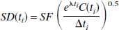
where SF is the scale factor that controls the level of noise, C(t_i) is the noise-free simulated radioactivity, Δt_i is the scan duration (seconds), and Λ is the radioisotope decay constant. This model is appropriate in the case of low or constant randoms fractions, constant scatter fraction, and relatively unchanging emission distribution with time.

Using Eq. 11, 1,000 noisy data sets were generated for each of several different values of SF. Different ranges of SF values (0.5–5 and 2–20 for [¹⁸F]FCWAY and [¹¹C]MDL 100,907, respectively) were selected for the two tracers given the body mass differences between humans ([¹⁸F]FCWAY) and monkeys ([¹¹ C]MDL 100,907), yielding roughly comparable noise levels. These SF values would cover the range of TAC noise found in a moderately sized region of interest to that of a pixel. The mean percent noise contained in the noisy data, which depends on both SF and the tracer half-life, was calculated as the ratio of the mean SD (Eq. 11) to the mean tissue activity (C(t)), and ranged from 1.9% to 18.8% for [¹⁸F]FCWAY and 1.9% to 18.6% for [¹¹C]MDL 100,907. The total distribution volume, V, was then estimated for these data sets by the linear (GA, TLS, MA1, and MA2) and nonlinear (KA) methods. The specific distribution volume, V_S, was also estimated by MA2 and KA. For GA, TLS, and MA1, t* was fixed at 42.5 minutes for [¹⁸F]FCWAY and 57.5 minutes for [¹¹C]MDL 100,907. These t* values were chosen graphically from preliminary GA of the noise-free data sets. Parameter estimation was considered “unsuccessful” when the methods failed (owing to ill conditioning or nonconvergence) or had V or V_S values < 0 or more than twice the true values. Furthermore, the estimation method was considered “unsuccessful” if at least 30/1,000 or 3% of the estimations were unsuccessful. V and V_S values were expressed as percent deviation from the true value or percent bias ± percent SD of the successful sample (n ⩽ 1,000). For unconstrained four-parameter fitting (KA), the initial parameter values were chosen randomly from the range of 75% to 125% of the true parameter value.

The asymptotic nature of Eqs. 1 and 2 was tested by examining the relationship between estimated V by the current analyses and the scanning duration for three sets of simulated noise-free [¹¹C]MDL 100,907 data. The sample mean K₁ (0.60543 mL·min⁻¹·mL⁻¹) and k₂ (0.0418 min⁻¹) values obtained in the basal ganglia of five monkeys by unconstrained 2T compartment fitting were used and V was fixed to 30 (mL/mL). Three different k₄ values were used for simulations representing the sample mean (0.0232 min⁻¹), the sample minimum (0.0123 min⁻¹), and one half of the minimum (0.0062 min⁻¹), the last value being chosen to exaggerate the asymptotic effect. A triexponential function was fitted to one of the original input functions and used to extrapolate it from 120 to 240 minutes. Using this extended input function and the parameter values, three noise-free TACs were generated for 240 minutes at 1-minute intervals. V was estimated 18 times by each of the current methods from these TACs, with scan duration successively shortened in 10-minute decrements from 240 to 70 minutes. For GA, TLS, and MA1, the latter fitting period of 60 minutes was used for these analyses; that is, t* was adjusted with the scan duration from 180 to 10 minutes.

Positron emission tomography study analysis

For the purpose of comparison with the simulated data analyses, examples from the human [¹⁸F]FCWAY and monkey [¹¹C]MDL 100,907 PET studies were used. [¹⁸F]FCWAY PET studies were performed in five normal human subjects, as described previously (Carson et al., 2000a). In brief, scans were acquired for 120 minutes (33 frames with scan duration ranging from 30 seconds to 5 minutes) after bolus administration of 6 to 10 mCi (specific activity, 800 to 1,600 Ci/mmol) of the tracer in three-dimensional mode on the GE Advance tomograph (GE Medical Systems, Waukesha, WI, U.S.A.). The arterial input function was determined from blood samples corrected for radiolabeled metabolites. Regional brain time activity data were corrected for tissue [¹⁸F]fluorocyclohexanecarboxylic acid, a principle metabolite that enters the brain (Carson et al., 2000b). Regional brain data for raphe (42 pixels, 4 mm²/pixel) and frontal cortex (500 pixels) were selected for the current analyses.

The [¹¹C]MDL 100,907 PET studies were performed in rhesus monkeys using 1% to 2% isoflurane anesthesia, as described previously (Watabe et al., 2000). In brief, control scans were acquired for 120 minutes (33 frames with scan duration ranging from 30 seconds to 5 minutes) after bolus administration of 20 to 39 mCi (specific activity, 700 to 1,800 Ci/mmol) of the tracer in two-dimensional mode on the GE Advance tomograph. The arterial input function was determined from the blood samples corrected for radiolabeled metabolites. In certain cases, [¹¹C]MDL 100,907 TACs could be well fit by a 1T model, particularly in regions with highest specific binding. For the purpose of evaluation of these linear estimation methods, five control studies were selected in which the regional brain data could be fitted reliably by the 2T model. Regional brain data for basal ganglia (84 pixels) and thalamus (42 pixels) were subjected to the current analyses. For these [¹¹C]MDL 100,907 studies, the first two frames (1 minute of data) were discarded for the estimation process in order to eliminate the intravascular radioactivity contribution. Correction for the time delay between the arterial input function and the brain time-radioactivity was applied as described by Watabe et al. (2000).

Mean percent noise contained in these samples was calculated based on deviations from 2T compartment fitting, with averaging done over the number of study subjects (n = 5). Distribution volumes were estimated by the current linear and nonlinear methods. V and V_S values were expressed as mean ± SD of the sample (n = 5). The values of t* were determined by performing GA with the modeling software PMOD (Burger and Buck, 1997), and these values were also used for corresponding TLS and MA1. An algorithm in PMOD searches for t* by performing LLS regression using data from t₀ (initialized to 0) to the end time and calculating for each data point the absolute error of regression; that is, |observed – predicted|/predicted value of the dependent variable. If the maximal value of this error within the fitting period is less than a prescribed value, then this t₀ is taken to be t*. Otherwise, this process is repeated, increasing t₀ successively until this condition is met (Burger and Buck, 1997). The prescribed value of 10% was used except for the raphe with [¹⁸F]FCWAY, for which a value of 20% was used because of the higher noise level in this small region of interest. The mean t* values were 52 ± 16 minutes (raphe) and 35 ± 7 minutes (frontal cortex) for [¹⁸F]FCWAY, and 34 ± 4 minutes (basal ganglia) and 29 ± 3 minutes (thalamus) for [¹¹C]MDL 100,907. A vascular radioactivity contribution of 4% was included in the unconstrained 2T compartment fitting.

Data analysis

All data analyses were implemented in MATLAB (The MathWorks, Natick, MA, U.S.A.) or PMOD (PMOD group, Zurich, Switzerland). Statistical analyses were performed with paired t-tests and the Pearson correlation analysis when applicable. Statistical significance was defined as P <0.05.

RESULTS

Simulation analysis

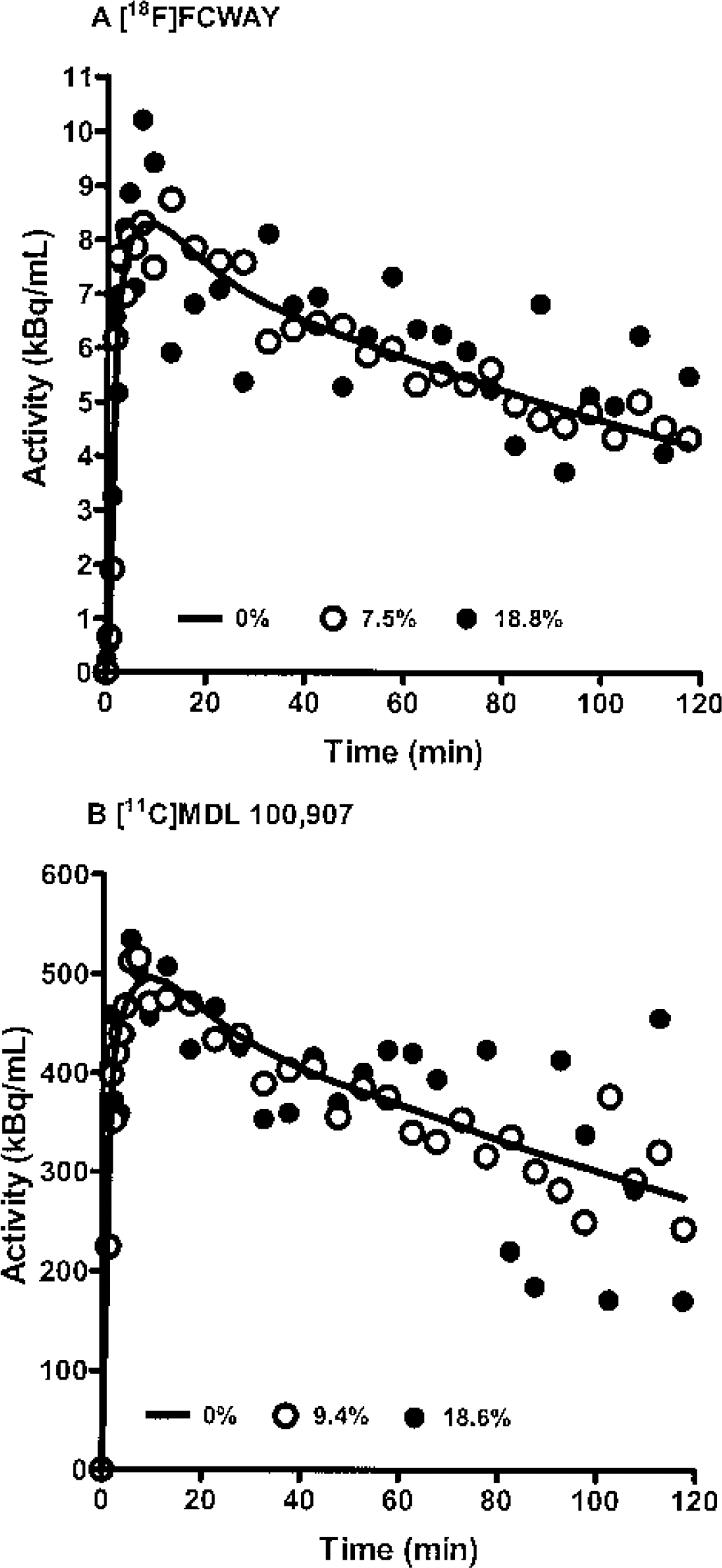
Figure 1 shows examples of TACs generated by simulations. The [¹¹C]MDL 100,907 TAC showed significantly more noise at late time points relative to the earlier time points than the [¹⁸F]FCWAY TAC, as produced by Eq. 11, which considers the decay half-life of the tracer (T_1/2 = 20.4 and 109.8 minutes for ¹¹C and ¹⁸F, respectively). Table 1 and Fig. 2 show the bias and variability of the estimation methods at different levels of noise for [¹⁸F]FCWAY and [¹¹C]MDL 100,907 (Table 1) and the average magnitude of percent bias and percent variability for [¹⁸F]FCWAY (Figs. 2A and 2B) and [¹¹C]MDL 100,907 (Figs. 2C and 2D), respectively.

Fig. 1.

Examples of simulated time-activity curves at mean noise of (A) 0%, 7.5%, and 18.8% for [¹⁸F]FCWAY (raphe) and (B) 0%, 9.4%, and 18.6% for [¹¹C]MDL (basal ganglia).

Fig. 2.

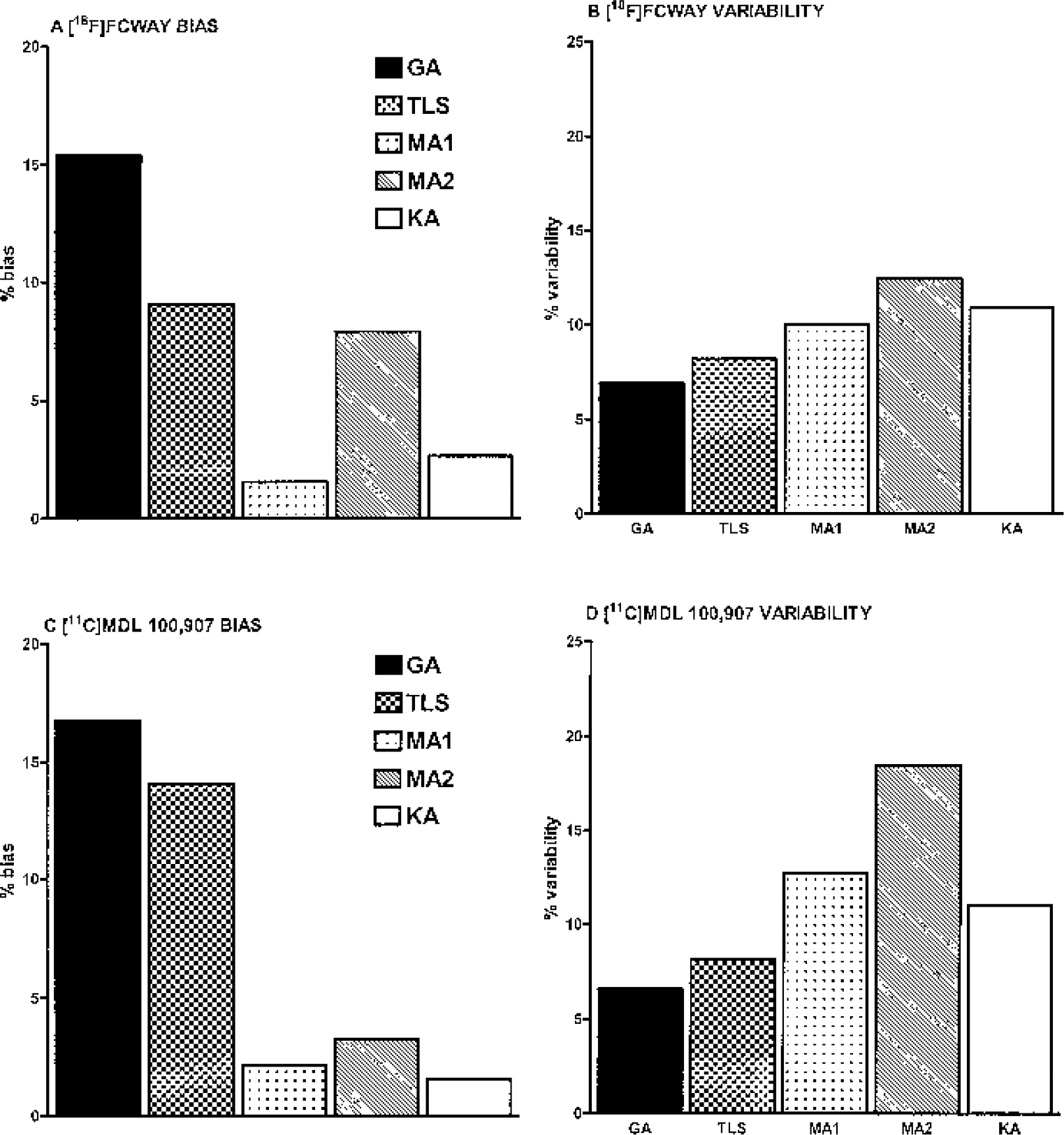
Bias and variability in estimating the total distribution volume, V, by different estimation methods for simulated [¹⁸F]FCWAY data (A and B) and [¹¹C]MDL 100,907 data (C and D). Values shown are averages over the simulated noise levels and biases are expressed as magnitude of percent biases (i.e., absolute percent biases). GA, graphical analysis; TLS, total least squares; MA1 and MA2, multilinear analysis 1 and 2; KA, kinetic analysis.

Table 1.

Bias and variability in estimating the total distribution volume by different estimation methods for simulated data at different noise levels

Tracer	Noise	GA	TLS	MA1	MA2	KA
[¹⁸F]FCWAY (“true” V value of 5.07 mL/mL)	1.9 (0.5)	−1.5 (1.8)	−1.1 (1.8)	−0.9 (1.8)	0.3 (1.8)	0.3 (1.8)
	3.8 (1)	−3.4 (3.4)	−2.0 (3.6)	−0.8 (3.5)	1.0 (3.6)	0.6 (3.6)
	7.5 (2)	−9.9 (6.1)	−5.0 (6.8)	−0.2 (7.1)	4.0 (8.2)	1.6 (8.2)
	11.3 (3)	−18.4 (8.5)	−9.9 (10.2)	1.2 (12.0)	10.0 (15.5)	3.9 (14.9)
	15.1 (4)	−26.1 (9.8)	−15.1 (12.2)	2.2 (15.4)	15.5 (19.7)*	4.5 (17.5)*
	18.8 (5)	−33.3 (11.9)	−21.3 (14.6)	3.9 (20.3)	16.6 (25.8)*	5.0 (19.5)*
	Average magnitude of % bias†	15.4	9.1	1.5	7.9	2.7
	Average % SD	6.9	8.2	10.0	12.4	10.9
[¹¹C]MDL 100, 907 (“true” V value of 34.9 mL/mL)	1.9 (2)	−2.8 (2.3)	−2.4 (2.4)	−1.7 (2.2)	−0.4 (2.1)	0.1 (2.0)
	4.7 (5)	−7.7 (5.3)	−5.9 (5.5)	−1.4 (5.3)	1.2 (5.7)	0.7 (5.6)
	9.4 (10)	−17.9 (8.0)	−14.0 (9.9)	0.7 (13.4)	6.5 (18.5)*	2.7 (12.3)
	14.0 (15)	−25.3 (8.6)	−21.2 (11.4)	3.9 (20.0)	7.2 (28.9)*	2.9 (16.7)*
	18.6 (20)	−30.1 (8.8)	−26.8 (11.6)	3.0 (22.6)*	1.0 (37.2)*	1.3 (18.6)*
	Average magnitude of % bias†	16.8	14.1	2.1	3.3	1.5
	Average % SD	6.6	8.2	12.7	18.5	11.0

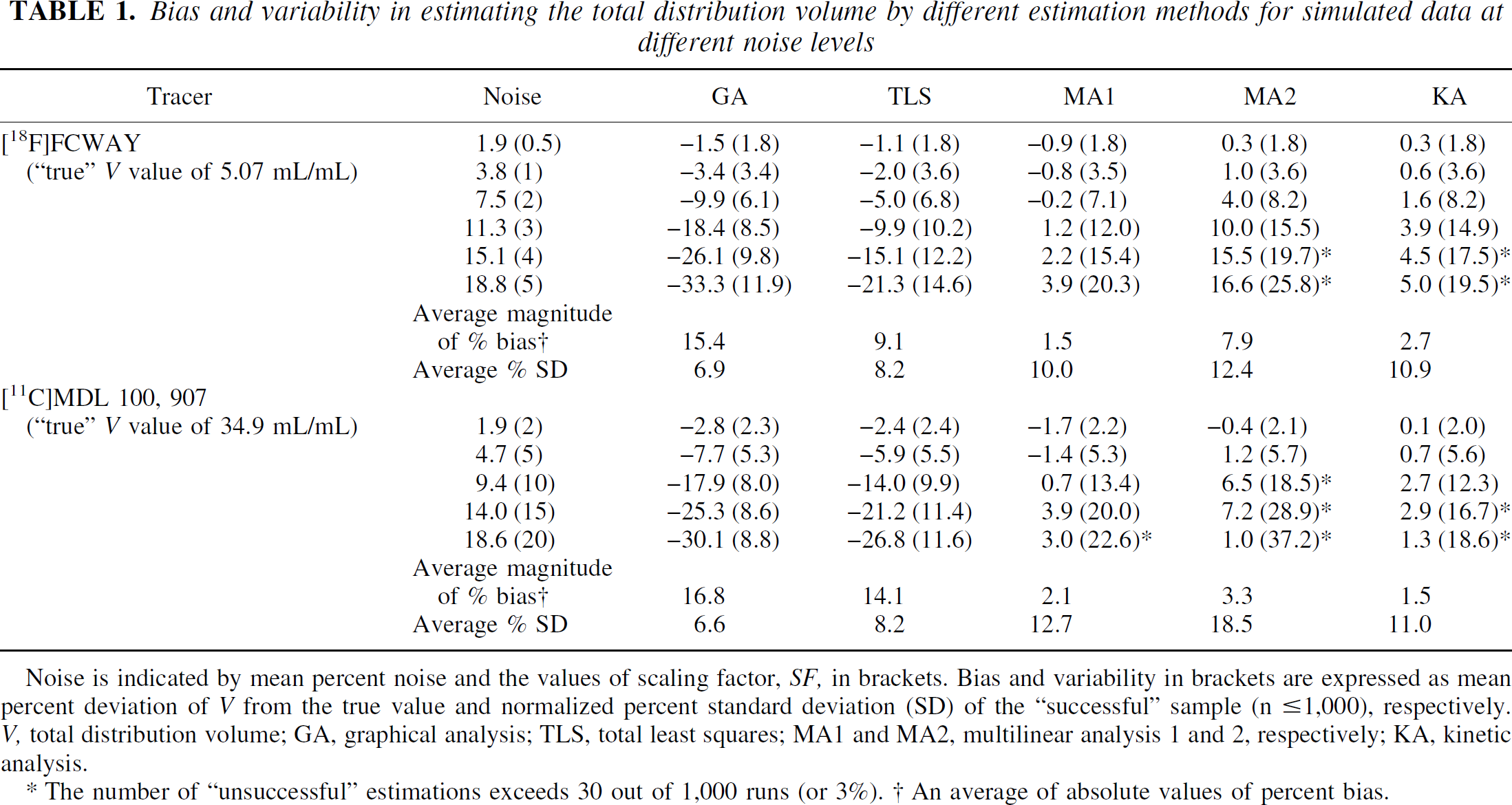
Noise is indicated by mean percent noise and the values of scaling factor, SF, in brackets. Bias and variability in brackets are expressed as mean percent deviation of V from the true value and normalized percent standard deviation (SD) of the “successful” sample (n ⩾ 1,000), respectively. V, total distribution volume; GA, graphical analysis; TLS, total least squares; MA1 and MA2, multilinear analysis 1 and 2, respectively; KA, kinetic analysis.

The number of “unsuccessful” estimations exceeds 30 out of 1,000 runs (or 3%). † An average of absolute values of percent bias.

Overall, the absolute biases were smallest for MA1 (0–4%), followed by KA (0–5%), MA2 (0–17%), TLS (1–27%), and GA (2–33%), whereas the variability was smallest with GA (2–12%), followed by TLS (2–15%), KA (2–20%), MA1 (2–23%), and MA2 (2–37%). The three linear methods (MA1, MA2, and TLS) all decreased the absolute bias of V estimates at the expense of increased variability compared with GA. These effects were most pronounced for MA1, moderate to large for MA2, and modest to moderate for TLS (Table 1 and Fig. 2). The bias and variability of KA was intermediate between MA1 and MA2 (Table 1 and Fig. 2). The increased variability of V estimates with increasing noise resulted in “unsuccessful” estimation rates at higher noise levels, particularly for MA2 and to a lesser extent for KA. MA2 was “unsuccessful” at the mean noise of 15.1% or greater for [¹⁸F]FCWAY and at 9.4% or greater for [¹¹C]MDL 100,907, respectively. KA was “unsuccessful” at these or one-level-higher noise and beyond (Table 1). Because unsuccessful estimations were excluded in calculating the mean biases, V estimation biases for MA2 or KA did not increase significantly or even decreased at the highest noise levels tested (Table 1).

The mean values of bias ± variability of V_S estimation over all noise levels by MA2 and KA were 5.9% ± 13.2% and 3.3% ± 11.6%, respectively, for [¹⁸F]FCWAY; and 5.8% ± 26.8% and 3.6% ± 14.5%, respectively, for [¹¹C]MDL 100,907. Thus, the bias and variability of V_S estimation by MA2 or KA was similar to those of V estimation by the respective method, with the bias and variability of MA2 somewhat inferior to those of KA.

Positron emission tomography study analysis

Figure 3 shows examples of unconstrained 2T compartment fitting of [¹⁸F]FCWAY data from the midbrain raphe (A) and [¹¹C]MDL 100,907 data from thalamus (B). Similar to the simulated results (Fig. 1), the [¹¹C]MDL 100,907 data showed more noise at late time points relative to the earlier time points than did the [¹⁸F]FCWAY data. The mean amounts of noise contained in the regional data were 11.0% ± 4.4% (raphe) and 3.5% ± 1.0% (frontal cortex) for [¹⁸F]FCWAY, and 1.9% ± 0.4% (basal ganglia) and 2.9% ± 0.3% (thalamus) for [¹¹C]MDL 100,907.

Fig. 3.

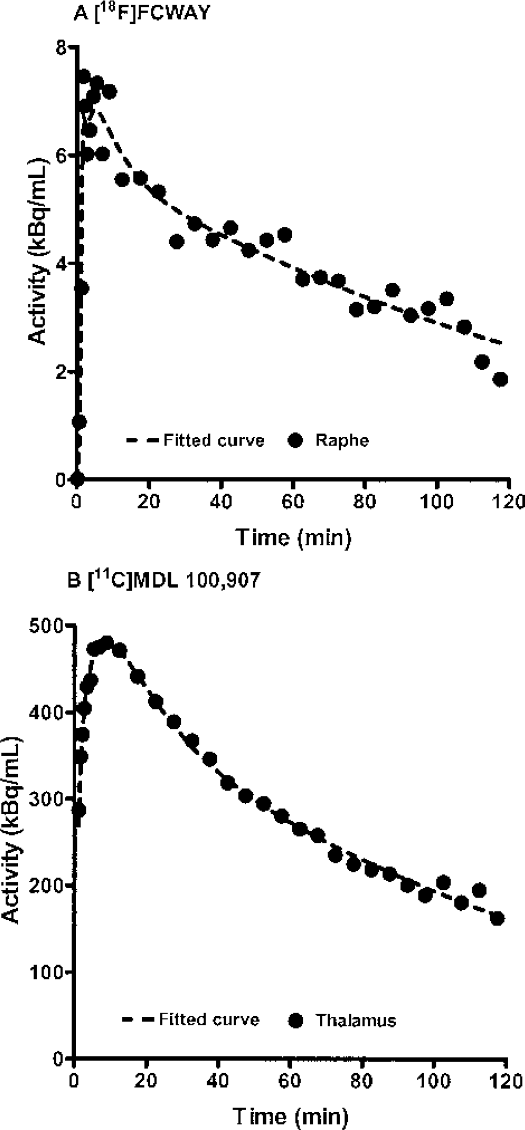
Example of unconstrained, 2T compartment fitting of actual (A) [¹⁸F]FCWAY (raphe) and (B) [¹¹C]MDL 100,907 (thalamus) positron emission tomography data.

Figure 4 depicts the mean regional values of V estimated by the different methods for [¹⁸F]FCWAY (Figs. 4A and 4B) and [¹¹C]MDL 100,907 (Figs. 4C and 4D). For [¹⁸F]FCWAY, the mean V values in the raphe (noise range, 8–19%) estimated by GA and TLS were lower by 24% ± 14% and 19% ± 13%, respectively, than those by KA (P < 0.05) and the mean V values estimated by TLS, MA1, MA2, and KA were all higher than those estimated by GA (P < 0.05), whereas there were no significant differences in the mean V values between the estimation methods in the frontal cortex (3.5% noise) (Figs. 4A and 4B). These results were consistent with the noise simulation results.

Fig. 4.

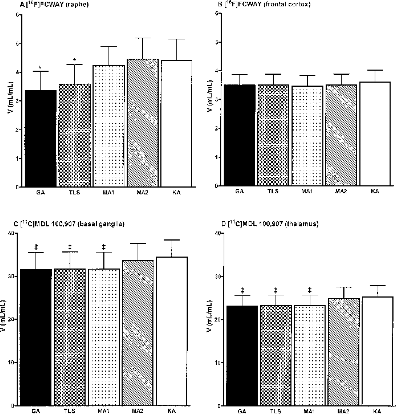
Sample mean distribution volume, V, by different estimation methods for [¹⁸F]FCWAY (A and B) and [¹¹C]MDL 100,907 (C and D). Error bars indicate SD (n = 5). *Significantly (P < 0.05) lower compared with KA. ‡Significantly lower (P < 0.05) compared with KA. GA, graphical analysis; TLS, total least squares; MA1 and MA2, multilinear analysis 1 and 2; KA, kinetic analysis.

For [¹¹C]MDL 100,907, there were no differences in the mean V values in the basal ganglia (2% noise) or thalamus (3% noise) between GA, TLS, and MA1, consistent with the simulation results. However, despite very low noise in the [¹¹C]MDL 100,907 data, the V values by GA, TLS, and MA1 were lower by 7% (range: 4–15%, P < 0.05) than those by MA2 or KA (Figs. 4C and 4D). The magnitude of this discrepancy tended to negatively correlate with the individual k₄ values (basal ganglia: mean = 0.0232 min⁻¹, range = 0.0123–0.0365 min⁻¹, r² = 0.62, P = 0.1; thalamus: mean = 0.0236 min⁻¹, range = 0.0176–0.0286 min⁻¹, r² = 0.46, P = 0.2) obtained by KA. The cause of this discrepancy was the fact that the automatic estimation process chose a value of t* that was earlier than the true point of linearity due to slow kinetics of [¹¹C]MDL 100,907. Figure 5 shows the relationship between scanning duration and V by GA, TLS, and MA1 for three sets of simulated noise-free [¹¹C]MDL 100,907 data extended to 240 minutes. GA, TLS, and MA1 equally and progressively underestimated V as t* and the scanning duration were successively decreased (Fig. 5A). As expected, MA2 and KA showed no such biases. This problem of choosing a t* value that is earlier than the true point of linearity would arise for tracers with slow kinetics, where the asymptotically linear portion of the graphical plot is achieved at late times (Fig. 5B).

Fig. 5.

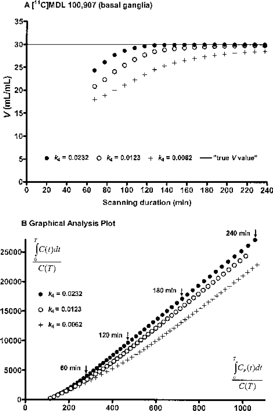
Relationship between scanning duration and distribution volume, V, by graphical analysis (GA), total least squares (TLS), and multilinear analysis 1 (MA1) for three sets of noise-free [¹¹C]MDL 100,907 data in the basal ganglia. In these simulations, k4 values are varied with the V value fixed at 30 mL/mL and the data are extended to 240 minutes (A), and corresponding graphical analysis plots (plotted every 5 minutes) (B) in which the plots are asymptotically linear. Arrows indicate points corresponding to 60, 120, 180, and 240 minutes.

Finally, there were no differences in the mean V_S values (mL/mL) between MA2 and KA. For [¹⁸F]FCWAY, the mean V_S values (mL/mL) were 3.9 ± 1.4 (MA2) versus 3.8 ± 1.5 (KA) in the raphe and 2.7 ± 0.6 (MA2) versus 2.9 ± 0.7 (KA) in the frontal cortex. For [¹¹C]MDL 100,907, values were 20.0 ± 8.1 (MA2) versus 21.3 ± 8.4 (KA) in the basal ganglia and 14.1 ± 6.2 (MA2) versus 14.1 ± 6.0 (KA) in the thalamus.

DISCUSSION

In the present study, we have shown that three alternative linear methods—TLS, MA1, and MA2—can reduce the magnitude of noise-induced bias of V estimates compared to GA for tracers with a 2T compartment configuration. Reductions in bias, however, come at the price of increased variability. Bias reductions are largest for MA1, moderate to large for MA2, and modest to moderate for TLS. The bias and variability of KA appear intermediate between MA1 and MA2. For tracers with early t*, MA1 appears to be the method of choice. For tracers with slow kinetics, however, selection of appropriate t* can be difficult and can lead to underestimation of V. Thus, in cases with low to moderate noise ranges, MA2, which uses the full data set, may provide the best balance between bias and computational ease suited for pixelwise parameter estimation.

For the unconstrained 2T model, variability of V estimates is smallest for GA. Thus, for the experimental paradigm in which reproducibility of pixelwise V measurements is of primary concern, GA may provide the most stable estimates of V in the presence of considerable statistical noise in the PET data at the expense of increased bias. Alternatively, region-of-interest based, as opposed to pixelwise, parameter estimation improves the signal-to-noise ratio; hence, MA1, MA2, or KA can provide parameter estimates with little bias and more acceptable variability.

Equation 1 for GA is model independent (Logan et al., 1990). This feature of GA is particularly useful for pixelwise parameter estimation for tracers where TACs from different regions are characterized by the 1T or 2T compartment configuration within the same PET data set. Both TLS and MA1 retain this feature. In fact, a method similar to MA1 effectively reduces the noise-induced bias in estimating V for the 1T model (Carson, 1993). Although Eq. 9 or A1 (Appendix) is derived from the 2T model, MA2 was also applicable to simulated data for the 1T model, where the bias and variability of MA2 was nearly identical to those of MA1 (data not shown). That is an interesting and surprising result because MA2 is an overdetermined model for data derived from a 1T model (i.e., there are too many parameters in the data). For nonlinear iterative fitting, this condition usually leads to convergence failures. For noise-free data, multilinear regression with Eq. 9 would also be expected to fail because the four “independent” variables are in fact linearly dependent. Two factors prevent this failure. First, the noise in the independent variables of Eq. 9 produces linear independence. Second, even with low-noise or noise-free data, small errors in the numerical integration of tissue and plasma data disrupt the linear dependence of these variables. Thus, with linear noniterative methods, the presence of poorly determined parameters did not affect the quality of the estimates of V. Thus, effectively, all of these alternative linear methods appear to be model independent. These noniterative linear methods are computationally simple, and therefore allow efficient pixelwise parameter estimation.

The GA, TLS, and MA1 equations are asymptotically linear. Therefore, the instantaneous slope of these equations is always less than but approaching V. This asymptotic linearity introduces a negative bias in estimating V, the magnitude of which depends on how the linear portion of the transformed data is defined (i.e., identification of t*). In the current simulation analysis (Table 1), the small initial negative bias for GA, TLS, and MA1 at low noise levels likely reflects this asymptotic linearity, because this bias can persist even for noise-free data, with its magnitude shrinking by pushing t* later). For GA, the time t* can be identified graphically (Logan et al., 1991). For MA1, this t* can also be identified graphically by plotting the observed versus predicted values of the dependent variable including all data points (Ichise et al., 1999). However, this task of graphically identifying t* accurately can be a challenge even with noise-free data (Fig. 5B). With noise added, identification of t* is more problematic. Alternatively, algorithms have been developed for automatic determination of t* (Burger and Buck, 1997; Watabe et al., 2000), which would be suited for pixelwise parameter estimation. For example, the algorithm developed by Watabe et al. (2000) automatically searches potential t* values to find the one with minimum coefficient of variation of V estimates. In PMOD, the criterion was to keep the maximum regression error below a predetermined value. These algorithms should be also applicable to TLS and MA1. Note that in this study, the t* values from GA were used for TLS and MA1 in order to allow direct comparison of the bias and variability results.

For the algorithm in PMOD to function properly, an appropriate predetermined value of maximum regression error must be selected by performing preliminary analysis, because the regression errors increase with noise. For example, for [¹⁸F]FCWAY, values of 10% and 20% were appropriate in the frontal cortex (3.5% noise) and raphe (11% noise), respectively. For [¹¹C]MDL 100,907, the t* values chosen by this algorithm in basal ganglia and thalamus (34 ± 4 and 29 ± 3 minutes, respectively) appear to be somewhat earlier than the true point of linearity as judged from the simulation analyses (Fig. 5), resulting in underestimation of V by GA, TLS, and MA1. The time points that gave minimum coefficient of variation of V were at 32 ± 8 and 22 ± 7 minutes for basal ganglia and thalamus, respectively. Thus, these automatic estimation algorithms can choose a value of t* that is earlier than the true point of linearity, particularly for tracers with slow kinetics if there are a small number of tissue data values acquired during the linear portion of the data. The underestimation of V by GA, TLS, and MA1 was reduced from 7.3% to 4.5% by using a fixed t* value of 60 minutes for all [¹¹C]MDL 100,907 subjects at the expense of increased standard errors of the V estimates. Thus, the requirement for defining the linear portion of the transformed data can be problematic for GA, TLS, and MA1, particularly with noisy data from tracers with slow kinetics. However, note that this problem of selecting t* applies only for tracers requiring the 2T model, because for the 1T model, both Eqs. 1 and 2 are linear for T > 0.

Equation 2 for MA1 has the potential theoretical advantage of using weighted least squares (WLS) to account for noise-level differences in C(T) (Carson, 1993). WLS requires that the time pattern of variance of noise be specified (Carson, 1986). Using the ideal weights, 1/Var [C(T)], for the current simulated data, WLS for MA1 improved the bias and variability of V estimation, minimally for [¹⁸F]FCWAY and slightly more for [¹¹C]MDL 100,907. For example, the bias and variability of V estimates were 0.4% and 11% with weighting and 0.9% and 13% without weighting, respectively, for [¹¹C]MDL 100,907 over all noise levels. Because there was a greater range in scan noise values for [¹¹C]MDL 100,907 due to the short half-life of ¹¹C, WLS would be expected to be more effective for [¹¹C]MDL 100,907 than for [¹⁸F]FCWAY. Therefore, WLS should improve the bias and variability of MA1 for tracers with nonuniform variance of noise. Caution should be exercised in applying WLS, however, because the presence of non-random errors for heavily weighted data points can lead to a biased estimation. For example, a heavy weight placed on early data points because of a low absolute level of noise can result in a large bias if there is an uncorrected time shift in the input function (Carson, 1993).

In contrast to GA, TLS, or MA1, MA2 has the advantage of not requiring the definition of t*; that is, MA2 can be applied to the full data set. In using the full data set, however, MA2 estimates four (or five with Eq. A1) parameters, as does kinetic analysis. Thus, it demonstrates similar or greater fitting instability for high noise ranges, as does KA (Table 1). Another potential advantage of MA2 is that, along with estimation of V, MA2 allows estimation of V_S with precision and accuracy comparable to that of unconstrained 2T nonlinear fitting, as shown in our results of simulation and actual PET data analyses. In most cases, the total volume of distribution, V = V_N + V_S, has been the more common outcome measure for the purpose of intersubject comparisons. V is useful under the assumption that the contribution of V_N to V is small, V_N is constant across subjects, or V_S can be estimated indirectly from V, provided that V_N is uniform and that V_N can be estimated from a region with no specific binding. For tracers with a significant intersubject or interregional variability in V_N, V_S could be a more appropriate measure of neuroreceptor binding, if it can be estimated reliably from an unconstrained fit. The physiologic interpretation of V_N and V_S obtained by any unconstrained 2T estimation method, however, should only be accepted following careful validation studies, since often the estimates of V_N are not uniform throughout the brain, but rather increase regionally with increasing V. For example, for the opiate antagonist [¹⁸F]cyclofoxy (Carson et al, 1993) and for [¹⁸F]FCWAY (Carson et al, 2000b), V_N (calculated as K₁/k₂ from unconstrained 2T fit) showed an approximately threefold variation across regions with positive correlation to V, whereas blocking studies showed minimal interregional variation in the level of nondisplaceable binding.

In OLS, two assumptions should be met. First, the independent variable is noise-free; and second, the dependent variable has uncorrelated random noise with mean zero. As shown by Slifstein and Laruelle (2000), GA produces a biased estimate of V with noisy data by violating these assumptions. The violation of the first assumption by Eq. 1 motivated the use of TLS in the present study, because TLS accounts for random noise with mean zero in the independent variable (Van Huffel and Vandewalle, 1991). In contrast, alternative multilinear methods MA1 (Eq. 2) and MA2 (Eq. 9 or A1) more closely satisfy these two OLS assumption by removing C(T) from the independent variable. As for assumption 1, Eqs. 1, 2, 9, and A1 have in the independent variable a single integral and additionally a double integral of C(t), in the case of Eq. 9 or A1. Typically the percent noise in these integral terms is much smaller than the percent noise in C(T). For example, the percent variations on a [¹⁸F]FCWAY TAC and its integral at 90 minutes generated with a SF value of 3 in our simulation study were 10.5% and 1.9%, respectively. Slight biases in calculating single and double integrals of the data from scan values can occur, however, because they are not instantaneous measurements but mean activity measurement over each scan.

For TLS, we have implemented the solution to the mixed OLS and TLS problem as described by Van Huffel and Vandewalle (1991). This solution was implemented for a problem with an arbitrary number of noise-free and noisy independent variables. In the special case of two independent variables, one constant and one with noise (as in Eq. 1), this is mathematically equivalent to solving for the regression parameters with a quadratic equation, as recently described by Varga and Szabo (2002) as the “perpendicular” regression model. We verified this mathematical equivalence by implementing the quadratic version of TLS and applied it to our simulated noisy data, and found that the two methods gave identical results. Thus, the “perpendicular” regression model of Varga and Szabo (2002) and our TLS model as applied to GA appear identical.

The use of TLS for Eq. 1 may not provide a perfect solution to the bias problem for the following two reasons. First, the structure of Eq. 1 causes the noise distribution of the dependent and independent variables to be correlated. Second, Eq. 1 can violate another assumption needed for TLS: that the noise distribution of the two variables has equal variance (Van Huffel and Vandewalle, 1991). Our results are consistent with these theoretical considerations of TLS; that is, TLS appears to have only modest to moderate effects on parameter bias.

Varga and Szabo (2002), however, showed dramatic reduction of noise-induced bias of the TLS-equivalent “perpendicular” regression method for three tracers with 2T compartment kinetics, [¹¹C]NNC 112, [¹¹C]-d-threo-methylphenidate, and [¹¹C](+) McN 5652. The reason for the discrepancy between their results and ours is not apparent. In both studies, tracers with different kinetic parameters were used, and the results were not dependent on tracer kinetics. The noise models and range of noise levels tested in both studies are very similar. A remaining difference is the input function. To address whether this function was the source of the discrepancy, we performed TLS simulations varying the terminal clearance rate of the input function. Although the value of the clearance rate somewhat altered the magnitude of the noise-induced bias, it did not remove the bias, as shown by Varga and Szabo (2002). Thus, the source of the inconsistency in these results remains unknown.

CONCLUSIONS

Three alternative linear methods to Logan GA have been evaluated as strategies to improve V estimates. TLS estimation accounts for noise in the independent variable, and MA1 and MA2 only have tissue concentration appearing as integrals in the independent variable(s). Our results from simulated and actual PET data of the 5-HT_1A tracer, [¹⁸F]FCWAY, and the 5-HT_2A tracer, [¹¹C]MDL 100,907, show that TLS, MA1, and MA2 all reduce the magnitude of noise-induced bias at the expense of increased variability compared with GA. These noniterative linear methods are computationally simple, and therefore allow efficient pixelwise parameter estimation. For tracers with kinetics that permit t* to be accurately identified within the study duration, MA1 appears to be the method of choice. However, for tracers with slow kinetics and for data with low to moderate noise ranges, MA2 may provide the lowest bias while maintaining the computational ease necessary for pixelwise parameter estimation.

Footnotes

APPENDIX

If the whole blood-to-plasma parent radioactivity is constant for the scanning period, the MA2 method can be extended to account for the presence of intravascular radioactivity. Assuming no radiolabeled metabolites in plasma, if the total volume of distribution (V*) is defined to include the plasma, then V* = V_N + V_S + V_P, where V_P (mL) is the regional plasma volume. The following equation, which corresponds to Eq. 9, can be then derived from Eqs. 5 and 6:

where γ₁ = k₂k₄V*, γ₂ = -k₂k₄, γ₃ = -(k₂ + k₃ + k₄), and γ₅ = V_P. Eq. A1 is a five-parameter version of Eq. 9, where V* is calculated as the ratio of the first two partial regression coefficients, −γ₁/γ₂. V_S is given by the equation

Acknowledgements

The authors thank Dr. Jeffrey Tsao for his excellent programming assistance in implementing the total least-squares algorithms in MATLAB, Mr. Douglass Vines for his assistance in data analysis, and the entire PET Department Staff for technical assistance.

References

Blomqvist

(1984) On the construction of functional maps in positron emission tomography. J Cereb Blood Flow Metab 4:629–632.

Burger

Buck

(1997) Requirements and implementation of a flexible kinetic modeling tool. J Nucl Med 38:1818–1823.

Carson

R.E.

(1986) Parameter estimation in positron emission tomography. In: Positron emission tomography. Principles and applications for the brain and the heart ( Phelps

M.E.

Mazziota

J.C.

Schelbert

H.R.

, eds), New York: Raven Press, pp 347–390.

Carson

R.E.

(1993) PET parameter estimation using linear intergration methods: bias and variability consideration. In: Quantification of brain function: tracer kinetics and image analysis in brain PET ( Uemura

Lassen

N.A.

Jones

Kanno

, eds), Amsterdam: Elsevier Science Publishers B.V., pp 499–507.

Carson

R.E.

Channing

M.A.

Blasberg

R.G.

Dunn

B.B.

Cohen

R.M.

Rice

K.C.

Herscovitch

(1993) Comparison of bolus and infusion methods for receptor quantitation: application to [18F]cyclofoxy and positron emission tomography. J Cereb Blood Flow Metab 13:24–42.

Carson

R.E.

Spanaki

M.G.

Herscovitch

Theodore

W.H.

Eckelman

W.C.

(2000a) Human 5-HT1A PET studies with [18F]FCWAY [abstract]. Neuroimage 11(suppl):S45.

Carson

R.E.

Lang

Watabe

Der

M.G.

Adams

H.R.

Jagoda

Herscovitch

Eckelman

W.C.

(2000b) PET evaluation of [18F]FCWAY, an analog of the 5-HT1A antagonist WAY 100635. Nucl Med Biol 27:493–497.

Evans

A.C.

(1987) A double integral form of the three-compartment model, four rate-constant model for faster generation of parameter maps [abstract]. J Cereb Blood Flow Metab 7(suppl 1):S453.

Feng

Wang

Huang

S-C

(1993) A study on statistically reliable and computationally efficient algorithm for the measurement of local cerebral blood flow with positron emission tomography. IEEE Trans Med Imag 12:182–188.

10.

Feng

Huang

S-C

(1996) An unbiased parametric imaging algorithm for nonuniformly sampled biomedical system parameter estimation. IEEE Trans Med Imag 15:512–518.

11.

Gjedde

(1982) Calculation of cerebral glucose phosphorylation from brain uptake of glucose analogs in vivo: a re-examination. Brain Res 257:237–274.

12.

Ichise

Fujita

Seibyl

J.P.

Verhoeff

N.P.

Baldwin

R.M.

Zoghbi

S.S.

Rajeevan

Charney

D.S.

Innis

R.B.

(1999) Graphical analysis and simplified quantification of striatal and extrastriatal dopamine D2 receptor binding with [123I]epidepride SPECT. J Nucl Med 40: 1902–1912.

13.

Ito

Nyberg

Halldin

Lundkvist

Farde

(1998) PET imaging of central 5-HT2A receptors with carbon-11-MDL 100,907. J Nucl Med 39:208–214.

14.

Lang

L.X.

Jagoda

Schmall

(1999) Development of fluorine-18-labeled 5-HT1A antagonists. J Med Chem 42:1576–1586.

15.

Logan

Fowler

J.S.

Volkow

N.D.

Wolf

A.P.

Dewey

S.L.

Schlyer

D.J.

MacGregor

R.R.

Hitzemann

Bendriem

Gatley

S.J.

(1990) Graphical analysis of reversible radioligand binding from time-activity measurements applied to [N-¹¹C-methyl]-(−)-cocaine PET studies in human subjects. J Cereb Blood Flow Metab 10:740–747.

16.

Logan

Fowler

J.S.

Volkow

N.D.

Ding

Y.S.

Wang

G.J.

Alexoff

D.L.

(2001) A strategy for removing the bias in the graphical analysis method. J Cereb Blood Flow Metab 21:307–320.

17.

Motulsky

H.J.

Ransnas

L.A.

(1987) Fitting curves to data using nonlinear regression: a practical and nonmathematical review. FASEB J 1:365–374.

18.

Patlak

C.S.

Blasberg

R.G.

Fenstermacher

J.D.

(1983) Graphical evaluation of blood-to-brain transfer constants from multiple-time uptake data. J Cereb Blood Flow Metab 3:1–7.

19.

Slifstein

Laruelle

(2000) Effects of statistical noise on graphic analysis of PET neuroreceptor studies. J Nucl Med 41:2083–2088.

20.

Van Huffel

Vandewalle

(1991) The total least squares problem: computational aspects and analysis. Philadelphia: Society for Industrial and Applied Mathematics, pp 1–300.

21.

Varga

Szabo

(2002) Modified regression model for the Logan plot. J Cereb Blood Flow Metab 22:240–244.

22.

Watabe

Channing

M.A.

Der

M.G.

Adams

H.R.

Jagoda

Herscovitch

Eckelman

W.C.

Carson

R.E.

(2000) Kinetic analysis of the 5-HT2A ligand [¹¹C]MDL 100,907. J Cereb Blood Flow Metab 20:899–909

Strategies to Improve Neuroreceptor Parameter Estimation by Linear Regression Analysis

Abstract

Keywords

MATERIALS AND METHODS

Theory

Total least squares

Multilinear analysis 1

Multilinear analysis 2

Simulation analysis

Positron emission tomography study analysis

Data analysis

RESULTS

Simulation analysis

Positron emission tomography study analysis

DISCUSSION

CONCLUSIONS

Footnotes

APPENDIX

Acknowledgements

References