Sage Journals: Discover world-class research

Abstract

[¹¹C](+)McN-5652 is an established positron emission tomography tracer used to assess serotonergic transporter density. Several methods have been used to analyze [¹¹C](+)McN-5652 data; however, no evaluation of candidate methods has been published in detail yet. In this study, compartmental modeling using a one-tissue compartment model (K₁, k″₂), a two-tissue compartment model (K₁ to k₄), and a noncompartmental method that relies on a reference region devoid of specific binding sites were assessed. Because of its low density of serotonergic transporters, white matter was chosen as reference. Parameters related to transporter density were the total distribution volume DV″ (=K₁/k″₂, one tissue compartment), DV_tot (=K₁/k′₁ (1 + k₃/k₄), two tissue compartments), and R_v (=k′₃/k₄, noncompartmental method). The DV″, DV_tot, and R_v values extended over a similar range and reflected the known pattern of serotonergic transporters. However, all parameters related to transporter density were markedly confounded by nonspecific binding. With regard to K₁, the one-tissue compartment model yielded markedly lower values, which were, however, more stable. The minimal study duration needed to determine stable values for the distribution volume was ∼60 minutes. The choice of the method to analyze [¹¹C](+)McN-5652 data depends on the situation. Parametric maps of R_v are useful if no information on K₁ is needed. If compartmental modeling is chosen, both the one- and the two-tissue compartment models have advantages. The one-tissue compartment model underestimates K₁ but yields more robust values. The distribution volumes calculated with both models contain a similar amount of information. None of the parameters reflected serotonergic transporter density in a true quantitative manner, as all were confounded by nonspecific binding.

Keywords

Positron emission tomography Kinetic modeling Serotonin transporter

Many psychiatric disorders and neurodegenerative diseases involve the serotonergic system. The serotonin transporter, which is located on the presynaptic side of the neuron, plays an important role in the regulation of serotonin concentrations in the synaptic cleft. At present, [¹¹C](+)McN-5652 is the most successful positron emission tomography (PET) tracer with which to assess serotonergic transporter density. Its usefulness has been demonstrated in animals (Suehiro et al., 1993a, 1993b; Szabo et al., 1995a) and humans (Szabo et al., 1995b, 1996). One of the drawbacks of the tracer is the relatively high fraction of nonspecific binding. Szabo et al. (1995b) measured nonspecific binding by blocking [¹¹C](+)McN-5652 uptake with fluoxetine and using the inactive enantiomer [¹¹C](−)McN-5652. Their work demonstrated that nonspecific binding accounts for ∼50% of tracer uptake in the thalamus, a structure with a high density of serotonergic transporters. With regard to methods of analysis, there are as yet no published reports that compare different methods. In one study, it is mentioned that of several tested compartmental models, a one-tissue compartment model yielded the most robust values (McCann et al., 1998), but no data were shown. Thus, the purpose of this study was to examine several methods of analysis. The chosen methods were compartmental modeling employing one- and two-tissue compartment models and the method developed by Ichise et al. (1996), which has the advantage that it does not require an arterial input function.

METHODS

Chemistry

The parent compound, McN-5652, was prepared starting from 2-phenylpyrrolidine and 4-methylthiomandelic acid in a five-step synthesis, as reported previously (Maryanoff et al., 1987; Sorgi et al., 1990). Enantiomerically pure (+)McN-5652 was obtained by crystallization of McN-5652 with (−)-di-p-toluyltartaric acid (Zessin et al., 1999). The transformation of (+)McN-5652 to the corresponding thioester precursor was achieved by S-demethylation with sodium amide at low temperatures (−78°C) followed by conversion of the intermediate thiol with acetyl chloride (Zessin et al., 1999). The radiosynthesis was accomplished by S-methylation with [¹¹C]methyl iodide of the thiol precursor, which was generated in situ from the thioester precursor by hydrolysis with potassium hydroxide at 40°C for 2 minutes, as previously reported (Zessin et al., 1999). Purification was performed with semipreparative high-performance liquid chromatography (Phenomenex Luna, [Brechbuehler AG, Schlieren, Switzerland], C18, 250 × 10 mm, 5 μm; 0.01 mol/L ammonium formate 25%, acetonitrile 75%). The collected product fraction was evaporated to dryness and reconstituted to an injectable solution (physiological saline and ethanol 90:10, containing 0.1% Tween 80). The final product was sterilized by filtration through a 0.22-μm filter. The radiochemical purity of [¹¹C](+)McN-5652 (>95%) was determined with high-performance liquid chromatography (Phenomenex Luna, C18, 250 × 4, 6 mm, 5 μm; 0.1 mol/L triethylamine 20%, acetonitrile 80%). The specific radioactivity at the time of injection was 77 ± 23 GBq/μmol, and the injected mass was 2.87 ± 1.76 mg (mean ± SD).

Study population

Eight healthy volunteers (mean age 25 years, range 22 to 30 years; 6 women and 2 men) were studied. None of the subjects had a history of neurologic disorders. The study was approved by the local ethical committee, and written consent was obtained from each volunteer.

[¹¹C](+)McN-5652 positron emission tomography

The PET studies were performed on a whole-body scanner (Avance; GE Medical Systems, Waukesha, WI, U.S.A.). This is a scanner with an axial field of view of 14.6 cm and a reconstructed in-plane resolution of 7 mm. After positioning of the volunteers on the scanner, catheters were placed in an antecubital vein for tracer injection and the radial artery for blood sampling. A 10-minute transmission scan was acquired for correction of photon attenuation. After the injection of 350 to 400 MBq of [¹¹C](+)McN-5652 as a slow bolus over 4 minutes, a series of 31 scans were initiated in three-dimensional mode (9 × 20, 4 × 30, 2 × 60, 4 × 120, 9 × 300, and 3 × 600 seconds, total study duration 90 minutes). For the determination of the arterial input curve, arterial blood samples were collected every 30 seconds for the first 6 minutes and then at later times with increasing intervals until the end of the study (90 minutes after injection). An aliquot of each sample was measured in a gamma-counter, and the plasma was analyzed to correct for metabolized radioligand activity. After centrifugation (at 3,500 rpm for 10 minutes), 1 mL of plasma was extracted twice with heptane. Fractions of organic and aqueous phases were counted in a gamma-counter to measure authentic tracer and metabolites. The validity of this procedure was tested by analyzing five samples until 10 minutes after injection with thin layer chromatography after concentration of organic and aqueous phases and dilution in dichloromethane (thin layer chromatography, silica gel 60, mobile phase methanol).

Data analysis

Models and parameters for transporter density. The investigated methods included standard compartmental modeling using an arterial input function and the method developed by Ichise et al. (1996), which does not require an arterial input function. Tracer kinetic modeling was performed using the models depicted in Fig. 1. They contain one and two tissue compartments. The notation using primes is borrowed from Koeppe et al. (1991). The meaning of the parameters is as follows:

FIG. 1.

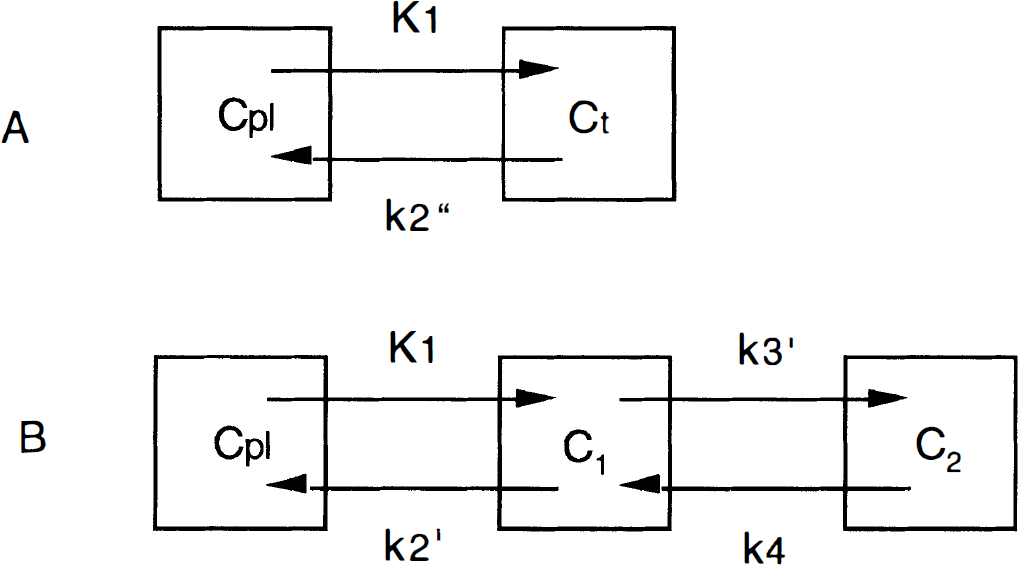
One- and two-tissue compartment models. C_pl, plasma concentration of authentic tracer; C_t, total tissue concentration.

K₁: describes uptake of tracer across the blood-brain barrier and is related to cerebral blood flow (CBF) and the first-pass extraction fraction (E_f; K₁ = CBF × E_f).

k″₂ and k′₂: represent back-diffusion from tissue to vascular space in the one- and two-tissue compartment model, respectively.

DV″: total distribution volume of tissue activity calculated with the one-tissue compartment model (K₁/k″₂).

DV_C1: distribution volume of compartment C₁ (K₁/k′₂).

DV_C2: distribution volume of compartment C₂ (K₁/k′₂k′₃/k₄).

DV_tot: total distribution volume of tissue activity calculated with the two-tissue compartment model [DV_C1 + DV_C2 = K₁/k′₂ (1 + k′₃/k₄)].

Tracer exchange between the compartments is described by the following differential equations:

\frac{d C_{1}}{d t} = K_{1} C_{p} - (k_{2}^{'} + k_{3}^{'}) C_{1} + k_{4} C_{2}

(1)

\frac{d C_{2}}{d t} = k_{3}^{'} C_{1} - k_{4} C_{2}

(2)

\frac{d C_{t}}{d t} = K_{1} C_{p} - k_{2}^{″} C_{t}

(3)

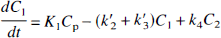
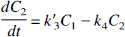
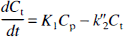
Equations 1 and 2 describe tracer exchange in the two-tissue compartment model and Eq. 3 in the one-tissue compartment model. As the total activity measured in a region is composed of counts from tissue and blood, all models contained a parameter (α) correcting for blood activity:

C_{voi} = (1 - α) C_{t} + α C_{blood}

(4)

where C_voi is PET counts in a volume of interest, α is percentage of intravascular space in tissue, C_t is activity in the extravascular compartment (with the two-tissue compartment model, C_t is the sum of C₁ and C₂), and C_blood is total blood activity. C_t was calculated by numerical integration of the differential equations; α was fixed at 0.05.

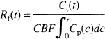
The Ichise method. This method was previously described in detail (Ichise et al., 1996). Its principle is to apply the Logan plot (Logan et al., 1990) to the time-activity curves of tissue with specific binding sites [C_t(t)] and of reference tissue devoid of specific binding sites [C_Ret(t)]. The input curve can then be algebraically eliminated, yielding the multilinear equation

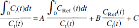
\frac{\int_{0}^{t} C_{t} (t) d t}{C_{t} (t)} = A \frac{\int_{0}^{t} C_{Ref} (t) d t}{C_{t} (t)} + B \frac{C_{Ref} (t)}{C_{t} (t)} + C

(5)

which can solved for A, B, and C using multilinear regression analysis. The parameter of interest is A. If DV_C1 in the reference and target regions is equal, it can be shown that

R_{v} = A - 1 = \frac{k_{3}^{'}}{k_{4}}

(6)

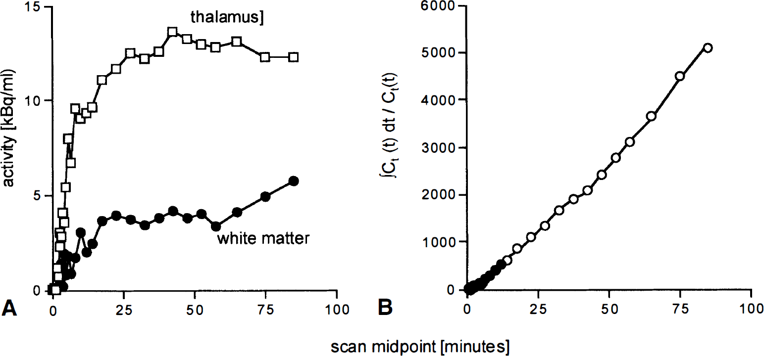
Considering the relations DV_C2 = K₁/k′₂k′₃/k₄ and DV_C1 = K₁/k′₂ yields that k′₃/k₄ (=R_v) = DV_C2/DV_C1. The big advantages of the Ichise method are that it does not require an arterial input function and that R_v can be calculated voxel-wise.

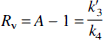
The unweighted least-squares solution of Eq. 5 was obtained by singular value decomposition (Flannery et al., 1992). Owing to the underlying Logan plot, the multilinear relationship (Eq. 5) holds only after some equilibration time. Therefore, initial points were omitted until the maximal difference between the remaining points and their regression estimates remained below 10%. When performing voxel-wise analyses, the longest omission time from the regional time-activity curves was adopted. In principle, there are no brain regions completely devoid of serotonergic transporters. Because of its low density of transporters, a white matter region was chosen as the reference region. An example of tissue data and the multilinear regression is illustrated in Fig. 2.

FIG. 2.

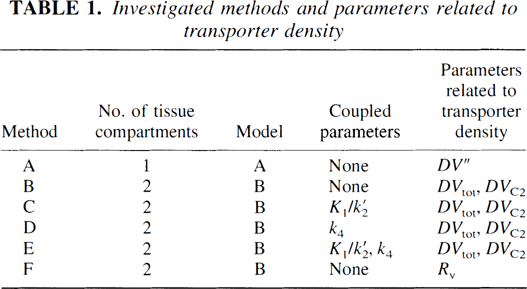
Analysis of Ichise et al. (1996) to calculate R_v. (A) Shown are the time-activity curves in thalamus and white matter, which serves as the reference region. (B) Shown is Eq. 5 evaluated at the scan midpoints (circles) and the model values obtained by multilinear regression (solid line). The data of the first 13 minutes (filled circles) have not been included in the regression to attain a match of <10% between data and model.

Candidate parameters related to the density of serotonergic reuptake sites and the associated methods are summarized in Table 1. Method A employs the one-tissue compartment model, and the only useful parameter for reuptake sites is the total distribution volume DV″. Methods B to E employ the two-tissue compartment model and several combinations of parameter coupling. The latter was described in detail previously (Buck et al., 1996). In short, if one assumes that certain parameters or combination of parameters are equal among different brain regions, it may be useful to perform a simultaneous fitting of all these regions with the constraint of common parameter values. In method C, it was assumed that DV_C1 was equal in all regions, in method D k₄, and in method E both DV_C1 and k₄. The coupling encompassed all 10 gray matter regions. Method F is the Ichise method described above. With the two-tissue compartment model, parameters related to serotonergic transporters were DV_tot and DV_C2.

TABLE 1.

Investigated methods and parameters related to transporter density

Method	No. of tissue compartments	Model	Coupled parameters	Parameters related to transporter density
A	1	A	None	DV″
B	2	B	None	DV_tot, DV_C2
C	2	B	K₁/k′₂	DV_tot, DV_C2
D	2	B	k ₄	DV_tot, DV_C2
E	2	B	K₁/k′₂, k₄	DV_tot, DV_C2
F	2	B	None	R _v

To get an independent estimate of the first-pass extraction fraction, the retention fraction (R_f) was calculated according to the following equation:

R_{f} (t) = \frac{C_{t} (t)}{C B F \int_{0}^{t} C_{p} (c) d c}

(7)

The denominator represents the total amount of extractable tracer delivered to a volume of interest up to time t. In case of no back-diffusion from tissue to vascular space (k′₂ = 0), R_f would be equal to the first-pass extraction fraction E_f. With back-diffusion, R_f will be smaller than E_f. Immediately after injection, back-diffusion is minimal and R_f will be a reasonable lower limit for E_f. The R_f was calculated for the thalamus at 3 minutes after injection and an assumed CBF of 0.7 mL/min/mL of tissue.

Positron emission tomography

Transaxial images of the brain were reconstructed using filtered back-projection (128 × 128 matrix, 35 slices, 2.34 × 2.34 × 4.25-mm voxel size). Photon attenuation was corrected for by means of a 10-minute transmission scan, and the data were corrected for decay. For the definition of volumes of interest, the scans from 10 to 90 minutes were summed and anatomical volumes of interest were defined over various cortical areas, the cerebellar cortex, the basal ganglia, the thalamus, and the pons. Tissue time-activity curves were then derived from these volumes of interest. The models were subsequently fitted to these time-activity curves using numerical integration of the operational equation (Eq. 4) and Marquardt's least-squares algorithm. The same volumes of interest were placed over the parametric maps of R_v, and the mean R_v in the volume of interest was used for comparison with the model-derived values. The placement of the volumes of interest, curve fitting, and calculation of parametric maps using the Ichise method were performed using the dedicated software PMOD (Mikolajczyk et al., 1998).

Assessment of methods

Several criteria were used to assess the methods. Goodness of fit of the different models was evaluated using F test statistics, the Akaike information criterion (AIC; Akaike, 1974), and visual inspection of the residuals.

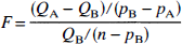
For the F test:

F = \frac{(Q_{A} - Q_{B}) / (p_{B} - p_{A})}{Q_{B} / (n - p_{B})}

(8)

The AIC is defined as follows:

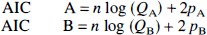
\begin{matrix} AIC & A = n log (Q_{A}) + 2 p_{A} \\ AIC & B = n log (Q_{B}) + 2 p_{B} \end{matrix}

(9)

In Eqs. 8 and 9, Q_A and Q_B represent the sum of squares for the fit with model A and B, respectively, p_A and p_B are the number of parameters of models A and B, and n is the number of data points. With the F test, an F value of >3.35 corresponds to a significant improvement using model B (P < 0.05). With AIC, model B is considered to lead to significantly better fits than model A if AIC B < AIC A.

The percentage coefficient of variation (COV) across the eight subjects was chosen as a measure for the stability of the estimated parameters: % COV = SD/mean × 100. The effect of study duration on parameter stability was estimated by consecutively shortening the fitting interval.

RESULTS

One-tissue versus two-tissue compartment model

Typical examples of tissue time-activity curves of thalamus and temporal cortex and the model fits using the one-tissue and the two-tissue compartment model with no parameter couplings among regions are provided in Fig. 3. In both regions, goodness of fit was improved with the two-tissue compartment model. The residuals indicate that the improvement is slightly more pronounced in the temporal cortex, the region with lower transporter density. This finding was confirmed by the quantitative analysis. Both the AIC and the F-test statistics demonstrated that the two-tissue compartment model yielded significantly improved fits in all regions (Table 2). For each region, significant improvements were found in at least six of the eight volunteers.

TABLE 2.

Significant improvement in fit by use of two-tissue compartment model, n = 8

	F-Test			AIC
	Mean F	SD	No. of subjects	Mean % reduction	SD % reduction	No. of subjects
Caudate	7.58	5.35	6	−5.89	5.36	7
Cerebellum	21.90	12.71	7	−19.78	10.69	8
Frontal	24.04	17.24	7	−21.48	12.03	8
Occipital	11.95	8.03	7	−10.01	6.25	8
Parietal	26.97	17.16	8	−21.92	10.09	8
Pons	9.81	8.33	6	−7.81	8.02	6
Putamen	12.11	9.01	6	−10.82	8.68	6
Temp-Med	20.28	21.48	8	−11.80	12.19	8
Temp-Lat	50.78	29.56	6	−34.32	10.37	6
Thalamus	18.54	11.69	7	−14.97	8.92	7

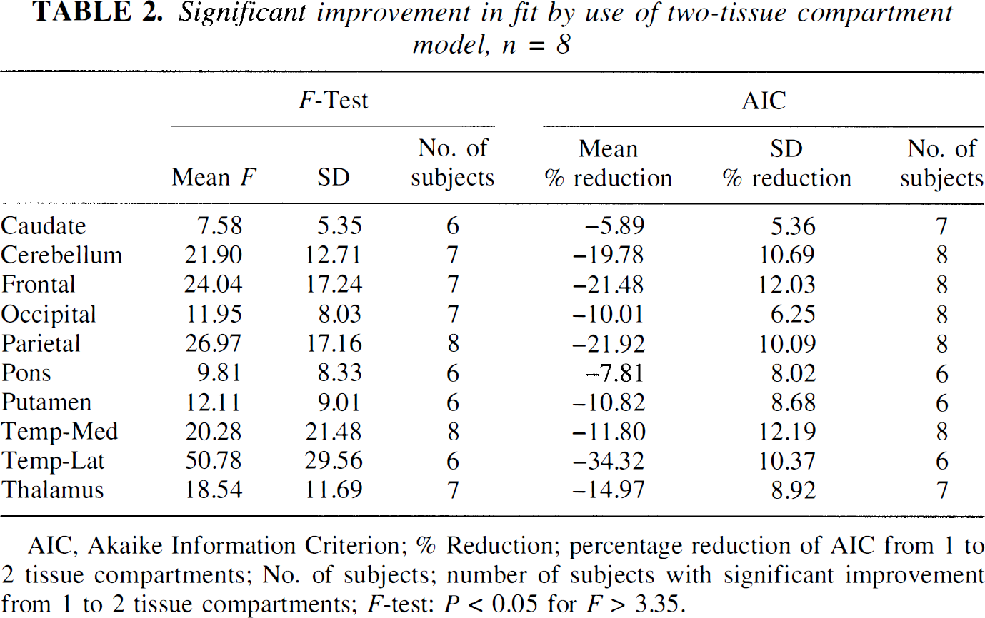
AIC, Akaike Information Criterion; % Reduction; percentage reduction of AIC from 1 to 2 tissue compartments; No. of subjects; number of subjects with significant improvement from 1 to 2 tissue compartments; F-test: P < 0.05 for F > 3.35.

FIG. 3.

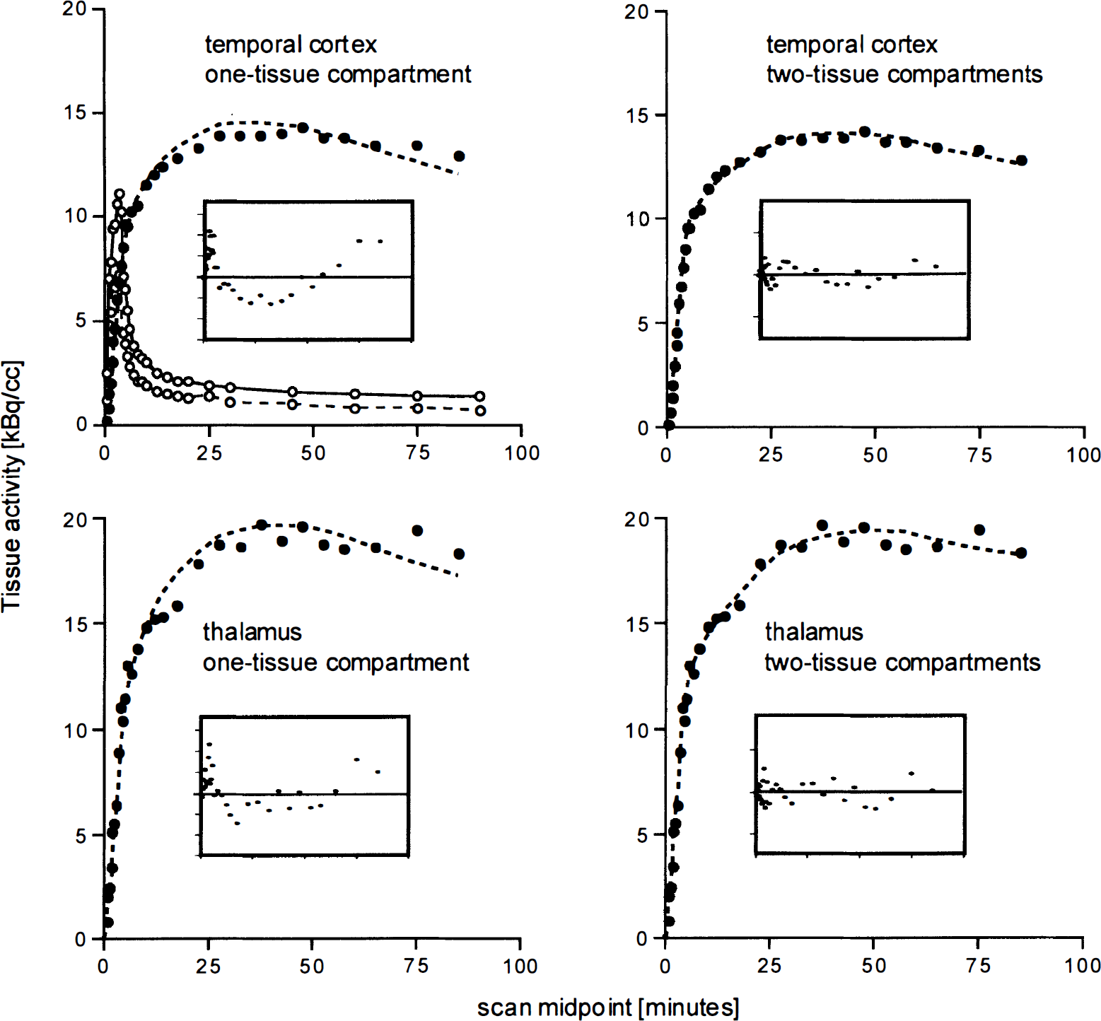
Measured tissue time-activity curves (filled circles) and model fit (dotted line) of thalamus and temporal cortex. The upper left panel additionally displays the time course of total plasma activity and authentic tracer. (Insets) Demonstrated are the residuals of model fit and measured values.

Comparison of transporter-related parameters derived from different two-tissue compartment models

The regional DV values and the percent COV as an indicator for parameter stability are listed in Table 3. In white matter, only the one-tissue compartment model yielded reasonable values. The ratio of DV in the regions with highest to the regions with lowest transporter density (high/low) ranged from 1.70 to 2.08. The values for percent COV are in the same range (26 to 40%) for DV″, DV_C2 calculated with no parameter coupling, and DV_tot.

TABLE 3.

Outcome measures related to transporter density

		DV″	DV _C2				DV _tot				R _v
		A	B	C	D	E	B	C	D	E	F
Caudate	Mean	20.69	22.33	20.38	19.72	18.95	24.22	23.00	23.06	21.74	2.17
	%COV	35.8	36.9	44.4	43.3	38.2	38.1	40.0	37.2	34.4	20.2
Thalamus	Mean	21.92	21.18	21.31	21.37	20.35	24.16	23.93	24.37	23.14	2.42
	%COV	27.8	33.4	31.1	34.0	29.4	27.0	28.5	26.8	26.4	17.8
Putamen	Mean	23.01	19.18	21.55	17.50	21.56	24.83	24.18	24.95	24.35	2.44
	%COV	36.2	32.9	38.0	44.5	38.4	33.7	34.3	33.8	35.3	21.6
Pons	Mean	17.82	16.69	16.63	16.96	16.21	19.55	19.25	19.35	19.00	1.56
	%COV	34.7	36.2	37.2	41.7	39.8	31.1	31.7	29.9	34.6	18.8
Temp-Med	Mean	15.16	15.57	14.85	14.22	13.30	17.59	17.47	16.88	16.10	1.38
	%COV	25.8	32.2	34.3	33.9	31.8	31.2	29.3	26.4	25.2	22.8
Parietal	Mean	12.79	12.12	11.00	11.84	11.02	13.98	13.63	13.78	13.81	1.13
	%COV	28.2	27.9	33.7	38.5	37.7	26.0	25.8	24.4	27.8	23.9
Temp-Lat	Mean	13.39	11.95	11.60	11.09	11.66	14.79	14.22	14.76	14.45	1.26
	%COV	28.9	29.8	36.0	36.8	36.4	25.4	28.2	29.1	28.4	27.4
Occipital	Mean	14.21	11.34	12.31	10.24	12.54	16.77	14.93	15.86	15.33	1.43
	%COV	33.6	35.7	40.1	40.2	40.8	44.1	32.0	34.1	33.4	28.8
Frontal	Mean	12.39	10.15	10.26	9.09	10.67	13.31	13.44	13.96	13.67	1.09
	%COV	29.4	40.9	39.0	54.5	39.7	28.0	26.7	28.4	28.1	40.6
Cerebellum	Mean	11.93	9.93	9.77	8.85	10.25	12.35	12.39	12.84	13.04	1.10
	%COV	28.5	32.3	38.1	48.4	38.8	28.6	28.1	28.0	28.2	37.7
White Matter	Mean	9.26	Unstable	Unstable	Unstable	Unstable	Unstable	Unstable	Unstable	Unstable
	%COV	0.2	Fits	Fits	Fits	Fits	Fits	Fits	Fits	Fits
	Mean %COV (across all regions)	30.3	33.3	36.6	40.5	36.5	31.4	30.5	29.8	29.6	27.7
	High/Low	1.70	1.99	1.96	2.08	1.82	1.73	1.74	1.70	1.65	1.95

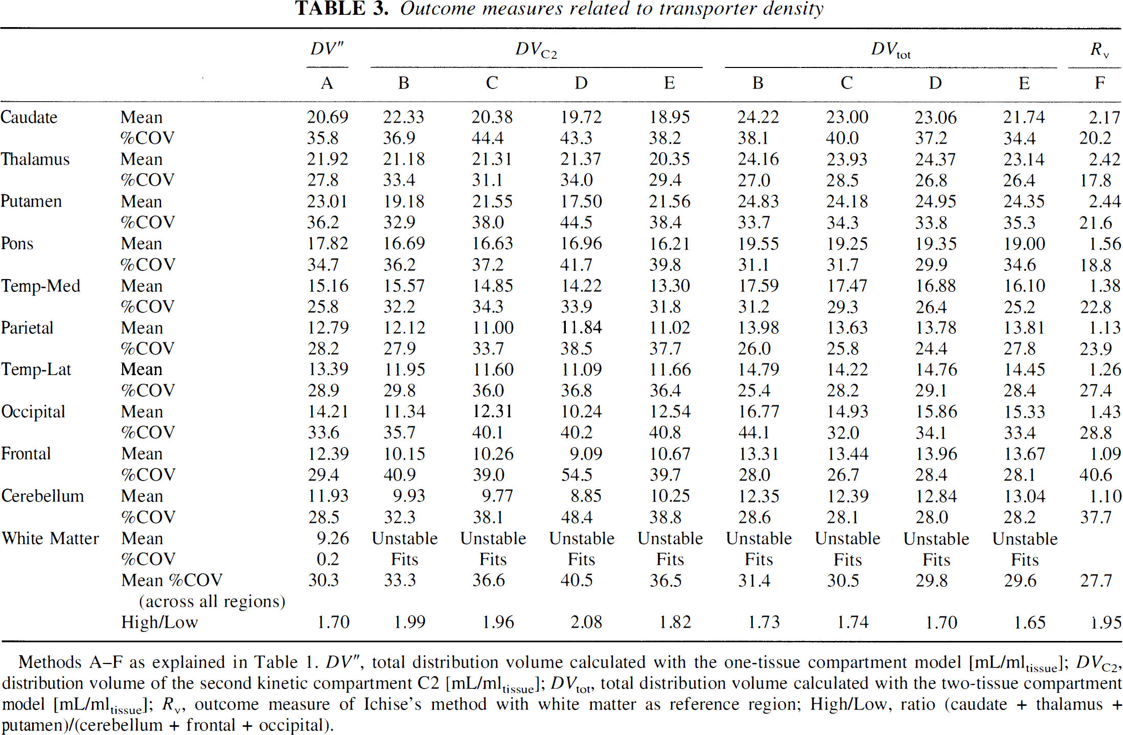
Methods A–F as explained in Table 1. DV″, total distribution volume calculated with the one-tissue compartment model [mL/ml_tissue]; DV_C2, distribution volume of the second kinetic compartment C2 [mL/ml_tissue]; DV_tot, total distribution volume calculated with the two-tissue compartment model [mL/ml_tissue]; R_v, outcome measure of Ichise's method with white matter as reference region; High/Low, ratio (caudate + thalamus + putamen)/(cerebellum + frontal + occipital).

None of the methods employing parameter coupling (methods C to E) yielded markedly lower values for percent COV for DV_C2 or DV_tot compared with method B with no parameter coupling. The parameter with the lowest percent COV turned out to be R_v (27.7%). The high/low ratio shows that the fractional increase from areas with low to areas with high transporter density was similar for R_v and DV_C2 and slightly lower for DV″ and DV_tot. The correlation of R_v and DV″, DV_tot, and DV_C2 is demonstrated in Fig. 4. There is generally a high correlation with Pearson's correlation coefficient r above 0.9. The intercept is close to zero for R_v versus DV_C2 and negative for R_v versus DV″ and R_v versus DV_tot.

FIG. 4.

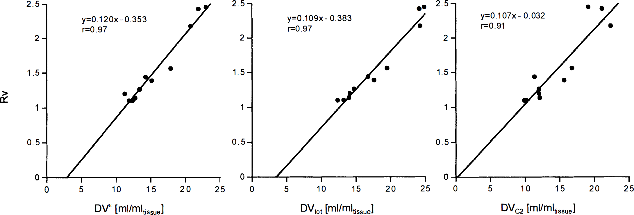
Correlation between R_v and DV. The linear regression was calculated using the mean of the regional values among the eight subjects. r, Pearson's correlation coefficient.

Parametric maps of R_v are demonstrated in the top row of Fig. 5. The images are of high quality, and the pattern of the R_v values reflects the known distribution of serotonergic transporters with high densities in thalamus, striatum, and midbrain. The contrast of R_v in these structures to cortex and cerebellum is considerably more pronounced than in the images of normalized uptake (bottom row).

FIG. 5.

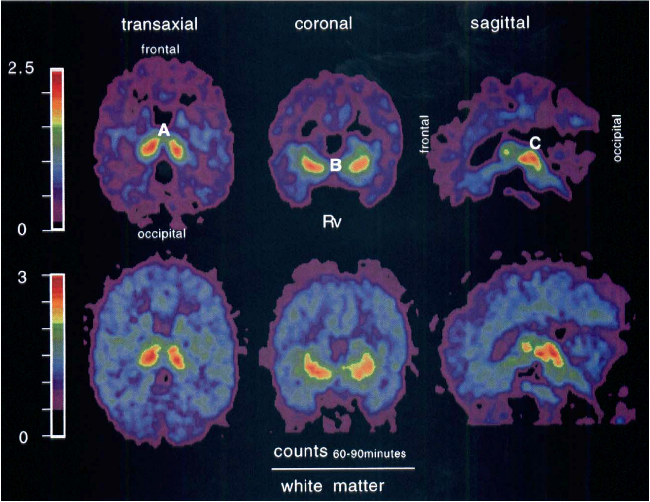
Images of R_v and tracer uptake normalized to white matter 60 to 90 minutes after injection. Note the high R_v values for thalamus (A; transaxial section), striatum (B; coronal section), and midbrain (C; sagittal section).

Stability of DV″ and DV_C2 versus study duration

Below 60-minute study duration, DV″ and DV_tot started to decline. With only 40 minutes of data included, DV″ dropped to ∼80% of its stable value. For study durations longer than 60 minutes, the values remained constant. Stable values of K₁ were reached for study durations longer than 50 minutes.

Tissue-to-plasma ratio

The time course of the ratio of regional activity to authentic tracer in plasma (Fig. 6; calculated with the model values derived from the two-tissue compartment model and a three-exponential fit to the declining part of the input curve) demonstrates that the ratio is continuously increasing in thalamus, cerebellum, and white matter.

FIG. 6.

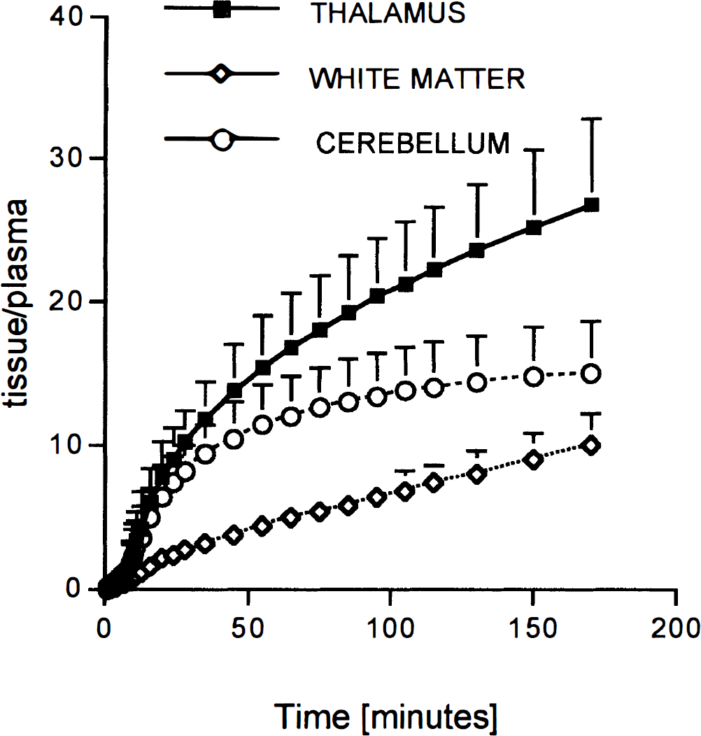
Time course of the tissue/plasma ratio. Tissue values were taken from the model fits at scan midpoint, and the plasma values were derived from a three-exponential fit to the declining part of the input function. Shown are the mean ± SD across the eight subjects.

Transport parameter K₁, DV_C1, and retention fraction

The values are summarized in Table 4. With the onetissue compartment model, the values of K₁ ranged from 0.25 (medial temporal cortex) to 0.39 (thalamus) mL/min/mL of tissue, and with the two-tissue compartment model (method B) from 0.39 (pons) to 0.68 (thalamus) mL/min/mL of tissue. In most regions, the values for DV_C1 were between 2 and 3 (method B). Coupling of DV_C1 among all regions (method C) yielded a value of 2.62 ± 67%. The retention fraction calculated with an assumed blood flow of 0.7 mL/min/mL of tissue in the thalamus at 3 minutes after injection was 0.93 ± 0.30 (mean ± SD across eight subjects).

TABLE 4.

K₁ values and distribution volume of the first kinetic compartment C1 (DV_C1)

		K₁One-tissue compartment	K₁Two-tissue compartment model				DV_C1Two-tissue compartment model
		A	B	C	D	E	B	C	D	E
Caudate	Mean	0.374	0.660	0.612	0.574	0.561	2.892	2.624	3.345	2.791
	%COV	34.9	59.6	69.2	59.9	64.3	109.3	67.2	86.4	70.7
Thalamus	Mean	0.394	0.683	0.624	0.617	0.571	2.987	2.624	3.002	2.791
	%COV	27.7	78.7	55.3	47.5	47.0	74.8	67.2	92.8	70.7
Putamen	Mean	0.386	0.555	0.585	0.587	0.563	5.653	2.624	7.450	2.791
	%COV	33.9	51.0	65.1	63.5	60.0	119.0	67.2	157.5	70.7
Pons	Mean	0.285	0.396	0.407	0.444	0.404	2.853	2.624	2.389	2.791
	%COV	38.1	54.9	69.3	74.7	70.7	84.4	67.2	105.9	70.7
Temp-Med	Mean	0.255	0.465	0.399	0.376	0.359	2.016	2.624	2.657	2.791
	%COV	33.6	65.3	66.9	51.0	56.9	65.9	67.2	90.1	70.7
Parietal	Mean	0.294	0.502	0.410	0.562	0.425	2.521	2.624	1.942	2.791
	%COV	26.6	85.6	47.3	56.1	49.8	88.4	67.2	128.6	70.7
Temp-Lat	Mean	0.316	0.491	0.459	0.577	0.473	2.840	2.624	3.678	2.791
	%COV	29.3	69.7	53.7	70.4	56.9	80.3	67.2	130.2	70.7
Occipital	Mean	0.352	0.581	0.503	0.557	0.523	5.427	2.624	5.621	2.791
	%COV	26.6	77.0	37.1	61.3	41.6	108.3	67.2	102.7	70.7
Frontal	Mean	0.326	0.493	0.447	0.701	0.493	2.769	2.624	4.175	2.791
	%COV	26.4	70.4	48.2	83.8	54.5	76.7	67.2	138.0	70.7
Cerebellum	Mean	0.350	0.482	0.492	1.651	0.577	2.415	2.624	3.985	2.791
	%COV	32.4	42.6	56.0	159.9	72.9	57.8	67.2	129.5	70.7
White Matter	Mean	0.098
	%COV	31.3
	Mean %COV (across all regions)	31.7	66.1	58.2	72.1	58.8	84.1	67.2	110.0	70.7

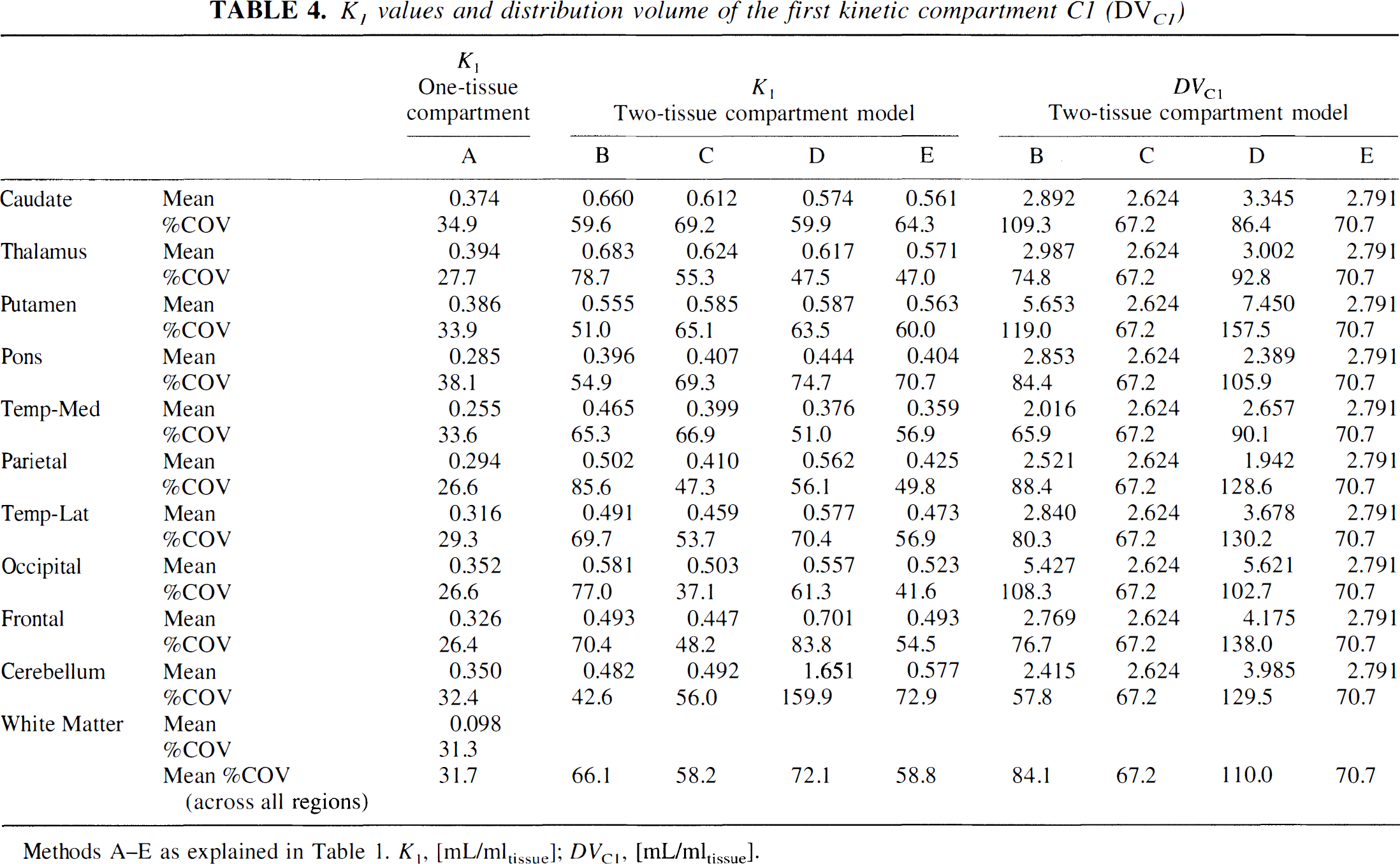
Methods A–E as explained in Table 1. K₁, [mL/ml_tissue]; DV_C1, [mL/ml_tissue].

DISCUSSION

One-tissue versus two-tissue compartment model

Several groups used the one-tissue compartment model to analyze [¹¹C](+)McN-5652 data. McCann et al. (1998) mention that they evaluated different compartmental models and found the one-tissue compartment model to yield the most robust values for DV″. With the one-tissue compartment model, DV″ is the only parameter related to transporter density. With the two-tissue compartment model, specific binding and nonspecific binding can potentially be separated. The significant improvement in the goodness of fit with the two-tissue compartment model indeed demonstrates that there are two distinguishable kinetic compartments. The important question is what they physiologically mean. Ideally, C₁ and C₂ would correspond to free plus nonspecific binding and specific binding, respectively. This is unfortunately not the case for [¹¹C](+)McN-5652. The DV_C2 is too large relative to DV_C1 to represent only specific binding. In the study of Szabo et al. (1995b), where nonspecific binding was directly measured by blocking specific binding with fluoxetine and by using the inactive enantiomer [¹¹C](−)McN-5652, the ratio of specific to nonspecific binding in the thalamus was on the order of 1. The ratio DV_C2/DV_C1 in this study in thalamus is ∼7. This demonstrates that DV_C2 is markedly overestimating specific binding, most likely because it is confounded by nonspecific binding. This interpretation also explains why the increase of DV_C2 from areas with low to areas with high transporter density underestimates the true increase. For instance, DV_C2 increased about twofold from cerebellum to thalamus, whereas the binding of [³H]paroxetine, a highly selective marker for the serotonergic transporter, demonstrated a fivefold increase in binding in thalamus compared with cerebellum (Laruelle and Maloteaux, 1989).

What is the preferred outcome measure for transporter density under these circumstances? The DV″, DV_tot, and DV_C2 all seem to be useful for the semiquantitative assessment of transporter density and the change in diseases or under pharmacological interventions or treatments. By semiquantitative, it is meant that the percentage change from one state to another does not correspond in a one-to-one fashion to the percentage change in transporter density. The high/low ratio is slightly lower for DV″ than for DV_tot or DV_C2 because the one-tissue compartment model is oversimplifying the kinetics. However, the difference seems to be too minor to clearly favor one or the other model. If specific binding per se were to be assessed, there would be several possibilities. Assuming that DV″ in white matter represents nonspecific binding, one could subtract DV″ in white matter from DV″ or DV_tot in the target region. The difference (DV_tot − DV_{white matter}″) was ∼14.9 in thalamus and 3.1 in cerebellum, yielding a ratio of 4.8. This is close to the ratio of ∼5 established with [³H]paroxetine (Laruelle and Maloteaux, 1989). If truly quantitative knowledge of nonspecific and specific binding is needed, one probably has to resort to blocking experiments or the additional use of the inactive enantiomer [¹¹C](−)McN-5652. However, as such protocols double the amount of tracer injections, they are impractical if one wants to make multiple assessments of transporter status in the same individual.

The relatively high amount of nonspecific binding and the impossibility of accurately determining specific binding will lead to reduced sensitivity to detecting changes in serotonergic transporter density. For instance, with 50% nonspecific binding, a reduction of 20% in transporter density would translate into a 10% reduction of DV″ and DV_tot. Another factor affecting the minimal change in transporter density that can reliably be detected is the test-retest accuracy of the method, which has not been determined yet.

With regard to K₁, the two-tissue compartment model yielded considerably larger values. Based on the retention fraction, they appear to be more in the physiological range. The latter was calculated to obtain a modelindependent estimation of K₁, using the relation K₁ = CBF × E_f and assuming that the retention fraction at early time points is a reasonable lower limit for the firstpass extraction fraction. The estimation of the retention fraction obviously depends on the assumed value of CBF, which was not directly measured. We chose a value in thalamus of 0.7 mL/min/mL of tissue. It is based on H₂¹⁵O PET measurements we previously performed in young volunteers (Buck et al., 1998b). Using this value and the measured retention fraction of 0.9 suggests that K₁ in thalamus should be on the order of 0.63 mL/min/mL of tissue. This is close to K₁ calculated with the two-tissue compartment model (0.68 mL/min/mL of tissue). In contrast, the one-tissue compartment model yielded a thalamic value of 0.39, suggesting considerable underestimation. On the other hand, the one-tissue compartment model yielded more stable values as the lower percent COV demonstrates. The choice of the model to calculate K₁ therefore depends on the situation. If robustness is the important issue, the one-tissue compartment model is still an option; if the values should be more quantitative, the two-tissue compartment model is preferable.

Parameter R_v calculated with Ichise method

This method seems the most attractive if no information of K₁ is required. In terms of percent COV and high/low range, R_v is comparable with DV″, DV_tot, and DV_C2. However, in contrast to compartmental modeling, the calculation of R_v does not require arterial blood sampling and therefore eliminates a source of error and discomfort for the patient or volunteer and the time-consuming determination of metabolites. It furthermore allows the voxel-wise calculation of R_v and its subsequent presentation as parametric maps (Fig. 5). An important question concerns the meaning of R_v in the present context. One has to bear in mind that R_v equals k′₃/k₄ (=DV_C2/DV_C1) if DV_C1 is equal in target and reference region and if DV_C2 is negligible in the reference region. Both conditions do not exactly hold with white matter as reference region. It was shown that white matter contains a minimal amount of serotonergic transporters (Laruelle and Maloteaux, 1989) and its DV_C1 may differ from the one of the target regions. The R_v will therefore not exactly represent the ratio DV_C2/DV_C1. However, the high correlation with DV″, DV_tot, and DV_C2 (Fig. 4) suggests that R_v is as useful as the DV value. The near zero intercept in the correlation with DV_C2 suggests that it is, in fact, directly proportional to DV_C2. The same limitations as discussed for DV_C2 obtained from compartmental modeling will therefore also hold for R_v.

Simple tissue ratios as measure for transporter density

If we assume that uptake in white matter is a reasonable estimate for nonspecific binding, one might ask whether the uptake ratio (target region/white matter) would not be a reasonable measure for transporter density. Such ratios are useful if they are measured at a precisely defined kinetic state, such as full kinetic equilibration between the compartments or at least “pseudoequilibration.” Full equilibration can be achieved only with an injection protocol that involves a constant infusion of the tracer. “Pseudoequilibrium” refers to a state after bolus injection when the ratio of the activity in the compartments reaches a stable value (Iyo et al., 1991). Another well defined state occurs when specific binding reaches a peak. At this time point, there is no net exchange between compartments C₁ and C₂ and the ratio of the counts in C₁ and C₂ reflects the true ratio at equilibrium (Farde et al., 1986). However, none of these states is reached with [¹¹C](+)McN-5652 after bolus injection. Neither is the difference (thalamus-white matter) as an estimate for specific binding reaching a peak (Fig. 6), nor is the ratio (thalamus/white matter) approaching a stable value. Simple tissue ratios therefore do not seem to be feasible measures for transporter density after bolus injection. They might, however, be an interesting option in protocols that try to achieve full equilibration. Such protocols have been successfully applied to other tracers (Abi Dargham et al., 1994; Buck et al., 1998a).

Minimal study duration and parameter coupling

Deleting successively more scans from the fitting procedure demonstrated that the minimal study duration is on the order of 50 to 60 minutes. Below that duration, DV values are underestimated. Parameter coupling is often an efficient method to increase the reliability of parameter estimates (Buck et al., 1996). In this study, parameter coupling did not lead to more reliable estimations of DV_tot or DV_C2 and is therefore not considered advantageous with [¹¹C](+)McN-5652. A likely reason may be that the assumptions of common parameters among regions may not hold. We argued above that the compartments C₁ and C₂ do not cleanly separate specific and nonspecific binding. Therefore, K₁/k₂′ will not accurately represent the DV of nonspecific binding and the assumption of a common K₁/k₂′ across regions may not be warranted.

CONCLUSION

The parameters DV″, DV_C2, DV_tot, and R_v contain a similar amount of information on serotonergic transporters. However, as all of them are confounded by nonspecific binding, none is reflecting transporter density in a fully quantitative manner. The choice of the method to analyze [¹¹C](+)McN-5652 PET data depends on the situation. If only a measure for serotonergic transporter density is required and no information on transport of tracer into the brain is needed, parametric maps of R_v calculated with the method of Ichise et al. (1996) seem to be the method of choice. The parameter R_v contains as much information on serotonergic transporter density as the DV values calculated with compartmental modeling. Compared with the latter, its calculation does not require arterial blood sampling and subsequent metabolite measurements and it can be determined on a voxel-wise basis. If information on K₁ is needed, the two-tissue compartment model yields values more in the expected physiological range. However, if robustness of K₁ is an issue, the one-tissue compartment model is preferable, although true K₁ values are underestimated. With regard to DV values, both models yield useful results, but the total distribution volume is slightly underestimated with the one-tissue compartment model.

Footnotes

Abbreviations used

Acknowledgements

The authors thank G. K. von Schulthess for the use of the PET infrastructure and Thomas Berthold for the data acquisition.

References

Abi Dargham

Laruelle

Seibyl

Rattner

Baldwin

Zoghbi

(1994) SPECT measurement of benzodiazepine receptors in human brain with iodine-123-iomazenil: kinetic and equilibrium paradigms. J Nucl Med 35:228–238

Akaike

(1974) A new look at the statistical model identification. IEEE Trans Automat Contr AC19:716–723

Buck

Westera

von Schulthess

Burger

(1996) Modeling alternatives for cerebral carbon-11-iomazenil kinetics. J Nucl Med 37:699–705

Buck

Frey

Blauenstein

Kramer

Siegel

Weber

(1998a) Monoamine oxidase B single-photon emission tomography with [¹²³I]Ro 43-0463: imaging in volunteers and patients with temporal lobe epilepsy. Eur J Nucl Med 25:464–470

Buck

Schirlo

Jasinksy

Weber

Burger

von Schulthess

(1998b) Changes of cerebral blood flow during short-term exposure to normobaric hypoxia. J Cereb Blood Flow Metab 18:906–910

Farde

Hall

Ehrin

Sedvall

(1986) Quantitative analysis of D2 dopamine receptor binding in the living human brain by PET. Science 231:258–261

Flannery

Press

Teukolsky

Vetterling

(1992) Numerical recipes in C. Cambridge: Cambridge University Press

Ichise

Ballinger

Golan

Vines

Luong

Tsai

Kung

(1996) Noninvasive quantification of dopamine D2 receptors with iodine-123-IBF SPECT. J Nucl Med 37:513–520

Iyo

Itoh

Yamasaki

Fukuda

Inoue

Shinotoh

(1991) Quantitative in vivo analysis of benzodiazepine binding sites in the human brain using positron emission tomography. Neuropharmacology 30:207–215

10.

Koeppe

Holthoff

Frey

Kilbourn

Kuhl

(1991) Compartmental analysis of [¹¹C]flumazenil kinetics for the estimation of ligand transport rate and receptor distribution using positron emission tomography. J Cereb Blood Flow Metab 11:735–744

11.

Laruelle

Maloteaux

(1989) Regional distribution of serotonergic pre- and postsynaptic markers in human brain. Acta Psychiatr Scand [Suppl] 350:56–59

12.

Logan

Fowler

Volkow

Wolf

Dewey

Schlyer

(1990) Graphical analysis of reversible radioligand binding from time-activity measurements applied to [N-¹¹C-methyl]-(–)-cocaine PET studies in human subjects. J Cereb Blood Flow Metab 10:740–747

13.

Maryanoff

McComsey

Gardocki

Shank

Costanzo

Nortey

(1987) Pyrroloisoquinoline antidepressants. 2. In-depth exploration of structure-activity relationships [published erratum in J Med Chem (1988) 31:276]. J Med Chem 30:1433–1454

14.

McCann

Szabo

Scheffel

Dannals

Ricaurte

(1998) Positron emission tomographic evidence of toxic effect of MDMA (“Ecstasy”) on brain serotonin neurons in human beings. Lancet 352:1433–1437

15.

Mikolajczyk

Szabatin

Rudnicki

Grodzki

Burger

(1998) A JAVA environment for medical image data analysis: initial application for brain PET quantitation. Med Inf 23:207–214

16.

Sorgi

Maryanoff

McComsey

Graden

Maryanoff

(1990) Asymmetric induction in an enammonium-iminium rearrangement. Mechanistic insight via NMR, deuterium labeling, and reaction rate studies. Application to the stereoselective synthesis of pyrroloisoquinoline antidepressants. J Am Chem Soc 112:3567–3579

17.

Suehiro

Scheffel

Dannals

Ravert

Ricaurte

Wagner

Jr (1993a) A PET radiotracer for studying serotonin uptake sites: carbon-11-McN-5652Z. J Nucl Med 34:120–127

18.

Suehiro

Scheffel

Ravert

Dannals

Wagner

Jr (1993b) [¹¹C](+)McN5652 as a radiotracer for imaging serotonin uptake sites with PET. Life Sci 53:883–892

19.

Szabo

Scheffel

Suehiro

Dannals

Kim

Ravert

(1995a) Positron emission tomography of 5-HT transporter sites in the baboon brain with [¹¹C]McN5652. J Cereb Blood Flow Metab 15:798–805

20.

Szabo

Kao

Scheffel

Suehiro

Mathews

Ravert

(1995b) Positron emission tomography imaging of serotonin transporters in the human brain using [¹¹C](+)McN5652. Synapse 20:37–43

21.

Szabo

Kao

Mathews

Ravert

Musachio

Scheffel

Dannals

(1996) Positron emission tomography of 5-HT reuptake sites in the human brain with C-11 McN5652 extraction of characteristic images by artificial neural network analysis. Behav Brain Res 73:221–224

22.

Zessin

Gucker

Ametamey

Steinbach

Brust

Vollenweider

(1999) Efficient synthesis of enantiomerically pure thioester precursors of [¹¹C]McN-5652 from racemic McN-5652. J Label Cpd Radiopharm 42:1301–1312

Evaluation of Serotonergic Transporters using PET and [ 11 C](+)McN-5652: Assessment of Methods

Abstract

Keywords

METHODS

Chemistry

Study population

[11C](+)McN-5652 positron emission tomography

Data analysis

Positron emission tomography

Assessment of methods

RESULTS

One-tissue versus two-tissue compartment model

Comparison of transporter-related parameters derived from different two-tissue compartment models

Stability of DV″ and DVC2 versus study duration

Tissue-to-plasma ratio

Transport parameter K1, DVC1, and retention fraction

DISCUSSION

One-tissue versus two-tissue compartment model

Parameter Rv calculated with Ichise method

Simple tissue ratios as measure for transporter density

Minimal study duration and parameter coupling

CONCLUSION

Footnotes

Abbreviations used

Acknowledgements

References

[¹¹C](+)McN-5652 positron emission tomography

Stability of DV″ and DV_C2 versus study duration

Transport parameter K₁, DV_C1, and retention fraction

Parameter R_v calculated with Ichise method