Voxel-Based Estimation of Kinetic Model Parameters of the l -[1- 11 C]Leucine PET Method for Determination of Regional Rates of Cerebral Protein Synthesis: Validation and Comparison with Region-of-Interest-Based Methods

Abstract

We adapted and validated a basis function method (BFM) to estimate at the voxel level parameters of the kinetic model of the l-[1-¹¹C]leucine positron emission tomography (PET) method and regional rates of cerebral protein synthesis (rCPS). In simulation at noise levels typical of voxel data, BFM yielded low-bias estimates of rCPS; in measured data, BFM and nonlinear least-squares parameter estimates were in good agreement. We also examined whether there are advantages to using voxel-level estimates averaged over regions of interest (ROIs) in place of estimates obtained by directly fitting ROI time-activity curves (TACs). In both simulated and measured data, fits of ROI TACs were poor, likely because of tissue heterogeneity not taken into account in the kinetic model. In simulation, rCPS determined from fitting ROI TACs was substantially overestimated and BFM-estimated rCPS averaged over all voxels in an ROI was slightly underestimated. In measured data, rCPS determined by regional averaging of voxel estimates was lower than rCPS determined from ROI TACs, consistent with simulation. In both simulated and measured data, intersubject variability of BFM-estimated rCPS averaged over all voxels in a ROI was low. We conclude that voxelwise estimation is preferable to fitting ROI TACs using a homogeneous tissue model.

Introduction

Biosynthesis of proteins is a fundamental process necessary for physiologic maintenance and functioning of organisms. In the central nervous system, de novo protein synthesis is critical for adaptive responses such as long-term memory formation. Animal studies indicate that regional rates of cerebral protein synthesis (rCPS) are altered in models of various clinical disorders (Qin et al, 2005; Smith and Kang, 2000; Widmann et al, 1991, 1992; Collins et al, 1980) and in certain physiologic states such as slow-wave sleep (Nakanishi et al, 1997). Regional rates of cerebral protein synthesis also change during brain development (Sun et al, 1995) and normal aging (Ingvar et al, 1985).

With the development and validation of the l-[1-¹¹C]leucine positron emission tomography (PET) method (Schmidt et al, 2005; Smith et al, 2005), fully quantitative measurement of rCPS in human subjects is now possible. We have implemented the method in awake, healthy young men and have shown that reproducible measurements of rCPS with low variability can be obtained (Bishu et al, 2008). Future applications are expected in studies of normal human brain, neurodegenerative diseases, and neurodevelopmental disorders that might be associated with dysregulation of cerebral protein synthesis (Bear et al, 2008).

Analysis of l-[1-¹¹C]leucine PET data in nonhuman primates (Smith et al, 2005) and human subjects (Sundaram et al, 2006; Bishu et al, 2008, 2009) has to date been carried out only at the region-of-interest (ROI) level. As ROI data are averaged over large numbers of voxels in the PET image, noise is reduced. Furthermore, computational time is minimal when the number of ROIs is small, and rCPS in each structure can be directly compared across subjects. With ROI analysis, however, any heterogeneity among voxels within the ROI is not taken into account. One consequence is that changes occurring in a subset of voxels within a ROI may be missed. To survey the entire volume, methods are needed to analyze each voxel within the image and generate maps of rCPS and other parameters of interest. Application of nonlinear least-squares (NLLS) estimation to each of the ~10⁷ voxels in a high-resolution PET image is infeasible, however, because of the high computational cost. In this study, we adapted and validated a basis function method (BFM) (Gunn et al, 1997) to estimate parameters of the [¹¹C]leucine kinetic model at the voxel level.

Although parametric maps are useful for surveying the brain volume and developing hypotheses regarding areas that may be affected in a particular condition, they cannot be used as generated for group statistical comparisons; spatial normalization to a common brain structure is required. In particular with high-resolution images, this process introduces uncertainty about the exact location in the brain with which each PET voxel should be associated. An alternative that avoids spatial normalization is to use parametric maps as the basis for computation of mean ROI parameter estimates. As the kinetic model parameters are not a linear function of measured activity, the mean of voxelwise estimates for a particular parameter will not, in general, equal the parameter estimated from the mean of the voxel activities, that is, from the ROI TAC. To determine whether voxelwise estimation confers any advantage for determining kinetic model parameters and rCPS in a ROI, we compared the mean of the voxelwise-estimated parameters with those determined from the ROI TACs. Comparisons between methods were carried out in simulations and in [¹¹C]leucine PET data acquired in healthy young men. The homogeneous tissue kinetic model for leucine (Schmidt et al, 2005) was used in the analyses.

Materials and methods

PET Studies

Data from previously reported studies (Bishu et al, 2008, 2009) of six awake, healthy male subjects (aged 20 to 24 years) were used for reanalysis in this study. The criteria for subject inclusion and the procedure for l-[1-¹¹C]leucine PET studies are described in detail in Bishu et al (2008). All studies were carried out on the ECAT High-Resolution Research Tomograph (HRRT, CPS Innovations, Knoxville, TN, USA), which has a spatial resolution of ~2.6 mm full width at half maximum (FWHM) (Wienhard et al, 2002). The 90-min emission scan was initiated coincident with a 2-min intravenous infusion of 25 to 30 mCi of l-[1-¹¹C]leucine (estimated specific activity 3 mCi/nmol). Images were reconstructed using the motion-compensated three-dimensional ordinary Poisson ordered subset expectation maximization algorithm (Carson et al, 2003) as 42 frames of data (16 × 15, 4 × 30, 4 × 60, 4 × 150, and 14 × 300 secs) and voxel size was 1.21 × 1.21 × 1.23 mm. Arterial blood sampling was carried out; concentrations of unlabeled and labeled leucine in arterial plasma and total ¹¹C and ¹¹CO₂ activities in whole blood were measured according to the methods detailed in Bishu et al (2008). All subjects underwent a T1-weighted magnetic resonance imaging of the brain for ROI placement.

Kinetic Model

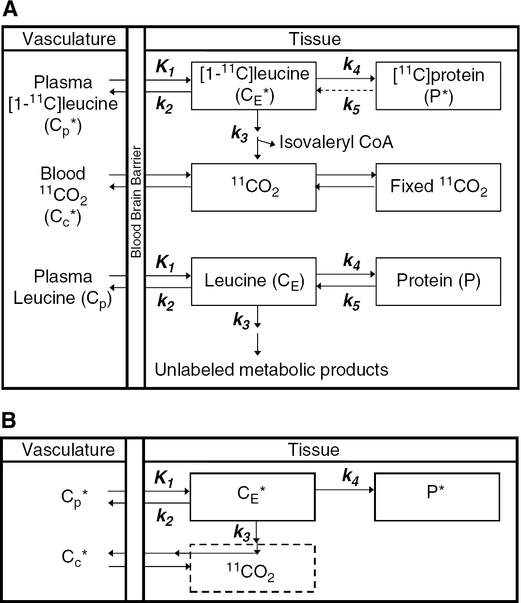
Figure 1A illustrates the kinetic model of the behavior of leucine in the brain (Schmidt et al, 2005). Total concentration of ¹¹C in the ROI or voxel (C_T*) includes free l-[1-¹¹C]leucine and l-[1-¹¹C]leucine incorporated into tissue protein (C_E* and P*, respectively), plus activity in blood (V_bC_b*, where V_b is the fraction of the ROI or voxel volume occupied by blood and C_b* the concentration of activity in whole blood). Total ¹¹C also includes labeled products of l-[1-¹¹C]leucine metabolism: ¹¹CO₂ and products of ¹¹CO₂ fixation. K₁ and k₂ are the rate constants for transport of leucine from plasma to tissue and vice versa, respectively. k₃ is the rate constant for the first two steps in leucine catabolism, transamination and decarboxylation, which yield ¹¹CO₂. k₄ and k₅ are the rate constants for leucine incorporation into protein and release of free leucine from proteolysis, respectively. It is assumed that there is no significant breakdown of labeled product during the experimental interval, that is, k₅P* ~0. The model used to describe labeled leucine holds also for unlabeled leucine, except that unlabeled leucine and protein are in steady state, and the steady-state breakdown of unlabeled protein (k₅P) is > 0. The model assumes that the tissue is homogeneous with respect to concentrations of amino acids, blood flow, rates of transport and metabolism of amino acids, and rates of incorporation into protein (Schmidt et al, 2005).

Figure 1

(A) Homogeneous tissue model for l[1-¹¹C]leucine PET method. Top rows illustrate the model used to describe the behavior of labeled leucine in the brain. K₁ and k₂ are the rate constants for transport of leucine from plasma to tissue and vice versa, respectively. k₃ is the rate constant for the first two steps in leucine catabolism, transamination and decarboxylation, which yield ¹¹CO₂. k₄ and k₅ are the rate constants for leucine incorporation into protein and for the release of free leucine from proteolysis, respectively. On account of the long half-life of protein in the brain (Lajtha et al, 1976), it is assumed that there is no significant breakdown of labeled product (P*) during the experimental interval, i.e., k₅P*~0. Labeled CO₂ arises either through catabolism of labeled leucine in the brain or through influx from the blood after catabolism in other tissue, and once in the brain it may be either transported back to the blood or fixed in the brain. Assuming no isotope effect, the rate constants for labeled and unlabeled leucine are identical. Thus, the model used to describe labeled leucine holds also for unlabeled leucine (bottom part of the figure), except that unlabeled leucine and protein are in steady state, and the steady-state breakdown of unlabeled protein, k₅P, is greater than zero. The model assumes that the tissue is homogeneous with respect to concentrations of amino acids, blood flow, rates of transport, metabolism of amino acids, and rates of incorporation into protein. Adapted from Schmidt et al, 2005. (B) Simplified homogeneous tissue model. Under the assumptions of negligible fixation of ¹¹CO₂ during the experimental period (Siesjö and Thompson, 1965) and rapid equilibration of ¹¹CO₂ between the brain and the blood (Buxton et al, 1987), the model reduces to two-tissue compartments (C_E* and P*) plus the ¹¹CO₂ compartment in which the concentration is known.

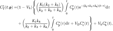
Under assumptions of negligible fixation of ¹¹CO₂ during the experimental period (Siesjö and Thompson, 1965) and rapid equilibration of diffusible ¹¹CO₂ between brain and blood (Buxton et al, 1987), the model simplifies to the homogeneous tissue model used in our analyses (Figure 1B). The concentration of ¹¹CO₂ in tissue is approximated by V_DC_c*, where C_c* is the ¹¹CO₂ concentration in whole blood and V_D the brain-blood equilibrium distribution volume of ¹¹CO₂. V_D was fixed at 0.41, the value measured in rhesus monkeys (Smith et al, 2005), which is in agreement with the mean whole brain-plasma equilibrium distribution volume determined from ¹¹CO₂ studies in humans (Brooks et al, 1984). (The blood-plasma equilibrium distribution volume is close to unity (Gunn et al, 2000).) Therefore,

$$C_T^{\ast }(t)=(1-V_b)\{C_E^{\ast }(t)+P^{\ast }(t)+V_D{C}_c^{\ast }(t)\}+V_b{C}_b^{\ast }(t).$$

(1)

In terms of rate constants

$$\begin{array}{rl}{C}_T^{\ast }(t;\mathit{\rho })=& (1-V_b)\{\left(\frac{K_1(k_2+k_3)}{k_2+k_3+k_4}\right)\underset{0}{\overset{t}{\int }}{C}_p^{\ast }(\tau )e^{-(k_2+k_3+k_4)(t-\tau )}d\tau \\ & +\left(\frac{K_1{k}_4}{k_2+k_3+k_4}\right)\underset{0}{\overset{t}{\int }}{C}_p^{\ast }(\tau )d\tau +V_D{C}_c^{\ast }(t)\}+V_b{C}_b^{\ast }(t),\end{array}$$

(2)

where dependence on the parameter vector ρ = [K₁, k₂ + k₃, k₄, V_b] is now shown explicitly.

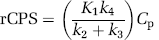
After rate constants have been estimated for a voxel or a ROI by one of the methods described below, rCPS can be calculated from the measured plasma concentration of unlabeled leucine, C_p, and estimated values of the rate constants as

$$\text{rCPS}=\left(\frac{K_1{k}_4}{k_2+k_3}\right)C_p$$

(3)

(Schmidt et al, 2005).

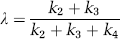
Equation (3) takes into account recycling of unlabeled amino acids derived from proteolysis, but the effects of recycling can also be examined. The factor Λ represents the fraction of unlabeled leucine in the precursor pool for protein synthesis derived from arterial plasma; the fraction derived from tissue proteolysis is (1-Λ). Lambda can be computed as

$$\lambda =\frac{k_1+k_3}{k_2+k_3+k_4}$$

(4)

(Schmidt et al, 2005).

Rate Constant Estimation

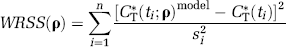
To estimate kinetic parameters from each ROI time-activity curve (TAC), weighted NLLS was used; it minimizes the weighted residual sum of squares (WRSS) objective function

$$WRSS(\mathit{\rho })=\sum _{i=1}^n\frac{[C_T^{\ast }(t_i;\mathit{\rho }{)}^{\text{model}}-C_T^{\ast }(t_i){]}^2}{s_i^2}$$

(5)

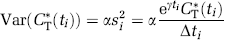
where n is the number of frames of data, C_T*(t _i ;ρ)^model is given by Equation (2), s _i ² is proportional to the variance of decay-corrected measured activity in the ROI, that is, C_T*(t _i ), and t _i the midpoint of the ith frame. Variance was modeled, assuming Poisson statistics, as

$$\text{Var}(C_T^{\ast }(t_i))=\alpha s_i^2=\alpha \frac{e^{\gamma t_i}{C}_T^{\ast }(t_i)}{\Delta t_i}$$

(6)

(Wu and Carson, 2002) where γ is the decay constant for ¹¹C, Δt _i the length of frame i, and α is a proportionality coefficient reflecting the noise level in the data. In PET data, α. is not known a priori, but its value does not affect the parameter estimates. We also evaluated the effect on parameter estimates of using weights based on whole brain activity instead of activity in the ROI itself for variance calculation by Equation (6). Results show that the effect is negligible; differences (in absolute value) in estimates of K₁, k₂ + k₃, k₄, and V_b were 0.4, 0.8, 0.6, and 0.6%, respectively, when averaged over all subjects and ROIs. For comparison with voxel-based estimates, weights based on whole brain activity were used. Nonlinear least-squares estimation was carried out with the Matlab^® function lsqcurvefit (The MathWorks, Natick, MA, USA) with initial conditions ρ₀= [0.0017 mL g⁻¹ sec⁻¹, 0.0033 sec⁻¹, 0.00083 sec⁻¹, 0.05]; iterations stopped when the change in ∥ &rh; ∥ < 10⁻⁸ or the change in WRSS < 10⁻⁶.

To estimate parameters at the voxel level, we implemented a BFM, as described below. For comparison, NLLS was also used for fitting of a subset of voxel data. In voxel-based estimation, activity in whole brain was used to calculate variance by Equation (6); this variance model was found to perform better than the one based on individual voxel values (Tomasi et al, 2008).

The difference between the tracer arrival time in the brain and the arterial sampling site was estimated by shifting blood curves 0 to 20 secs, fitting the whole brain TAC, and selecting the delay that produced the smallest WRSS. Tracer appearance times in various parts of the brain differ from the mean of the brain as a whole by ± 2 secs (Iida et al, 1988); therefore, in each study, for all regions and voxels, whole brain tracer arrival delay was used.

Basis Function Method

The use of NLLS is not feasible when working at the voxel level because of its high computational burden. A fast tool to estimate parameters is provided by the BFM. The method is based on a grid search approach and linear least-squares estimation, which was first introduced for determining regional cerebral blood flow (Koeppe et al, 1985). One observes from Equation (2): if the value of β = k₂ + k₃ + k₄ were known, Equation (2) would be linear in the coefficients, which could be quickly estimated using standard weighted linear least squares. The idea of the BFM is to define a grid of values for β in the physiologic range. For each β, the linear coefficients of Equation (2) are estimated and WRSS computed. The value of β and the coefficients at which WRSS is minimal are used to compute the model parameters. Details are given in Appendix A.

For our data set, 100 values spaced equally between β min = 0.0001 min⁻¹ and β_max = 0.5 min⁻¹ were used initially as the grid for β; this widely covers the range of physiologic values expected for k₂ + k₃ + k₄ (Bishu et al, 2008). Dependence of performance on the number and distribution of basis functions was tested using grids with 100 or 200 values, uniformly or logarithmically distributed, between β_min and β_max.

With the BFM approach, one or more parameter estimates may be negative for a given voxel. Rather than exclude these voxels from the analysis, which would likely create problems when considering ROI/voxel correlation, we developed the strategy presented in the appendix of reanalyzing each voxel that had one or more negative parameters after the initial BFM estimation. A voxel was discarded from further analysis only if reanalysis failed to produce non-negative parameter estimates.

Performance of Basis Function Method for Voxel Analysis

Basis function method performance for voxel analysis was assessed in both simulated and measured PET data. For simulation, values of parameters within the range of those previously estimated for cerebellar, cortical, and subcortical regions (Bishu et al, 2008), that is, K₁ = 0.05 mLg⁻¹ min⁻¹, k₂+ k₃ = 0.15 min⁻¹, k₄ = 0.04 min⁻¹, and V_b = 0.05, were used together with measured plasma and blood curves of one subject to generate a noiseless TAC according to Equation (2). Gaussian noise, with zero mean and variance computed by Equation (6), was added to obtain simulated noisy TACs at four different noise levels, namely α = 100, 1, 000, 2, 000, or 5, 000. In the same subject from whom we derived the input functions, the median estimates of α (WRSS/(n-p), where n is the number of data frames and p the number of parameters; Landaw and DiStefano, 1984) over all voxels in the thalamus, corona radiata, and the central nine slices of frontal cortex were 1, 763, 920, and 2, 591, respectively; this suggests that α = 1, 000 and 2, 000 are representative of noise levels found in l-[1-¹¹C]leucine voxel data measured on the HRRT. For each noisy TAC, BFM was used to estimate kinetic model parameters; weights for estimation were based on the whole brain TAC for this subject. For each noisy TAC, parameters were also estimated by NLLS. We refer to this as ‘single voxel simulation’ to distinguish it from the one described in the next section.

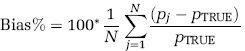
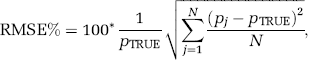
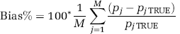
To assess BFM or NLLS performance at the voxel level, percent bias (Bias%) and percent root mean square error (RMSE%) were computed as

$$\text{Bias}\%={100}^{\ast }\frac{1}{N}\sum _{j=1}^N\frac{(p_j-p_{\text{TRUE}})}{p_{\text{model}}}$$

(7)

and

$$\text{RMSE}\%={100}^{\ast }\frac{1}{p_{\text{TRUE}}}\sqrt{\sum _{j=1}^N\frac{(p_j-p_{\text{TRUE}}{)}^2}{N}},$$

(8)

where p, is the BFM or NLLS estimate of a given rate constant at the jth noise realization and N = 1, 000 is the number of repetitions. Simulated voxels discarded from BFM analysis, those for which NLLS did not converge, and those for which any estimated parameter >1, were not included in computation of Bias% and RMSE%. In all cases, the fraction of voxels excluded was recorded.

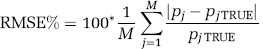
In a subset of measured data (one image plane each from two PET studies, ~20, 000 total voxels), parametric maps generated by BFM and NLLS were compared. In this case, in the absence of ‘true’ values, NLLS estimates were regarded as the gold standard. Average Bias% and RMSE% were computed for each parameter estimate as

$$\text{Bias}\%={100}^{\ast }\frac{1}{M}\sum _{j=1}^M\frac{(p_j-p_{j\text{TRUE}})}{p_{j\text{TRUE}}}$$

(9)

and

$$\text{RMSE}\%={100}^{\ast }\frac{1}{M}\sum _{j=1}^M\frac{|(p_j-p_{j\text{TRUE}})|}{p_{j\text{TRUE}}}$$

(10)

where p_jTRUE and p _i indicate the estimate of a given rate constant at the jth voxel determined by NLLS and BFM, respectively; M the total number of voxels. Notice that Equation (10) can be derived as the mean value of RMSE% given in Equation (8) when N = 1. To avoid having outliers unduly influencing results, (p _j - p_jTRUE)/P_jTRUE in Equation (9) was bounded between −1 and 1, and the threshold for the upper bound of │p _j -p_jTRUE│ /p_jTRUE in Equation (10) was set at 1. Furthermore, to avoid division by zero or near zero, voxels in which the NLLS estimate of either V_b or k₄ < 10⁻⁴ were excluded. This avoids, for example, including in the average a 100% bias for a voxel in which k₄(NLLS) = 10⁻⁶ and k₄(BFM) = 10⁻⁵, both estimates effectively zero.

Region of Interest Analysis

For use with measured PET data, ROIs were placed on each subject's magnetic resonance image by visually identifying anatomic landmarks, manually outlining the region, and constructing a binary mask to identify voxels in the region. The set of voxels in the PET image belonging, wholly or fractionally, to a given ROI was defined in the following way. The magnetic resonance image was aligned to the average 30 to 60 mins PET image by the use of Vinci software (Volume Imaging in Neurological Research, Max Planck Institute for Neurological Research, Cologne, Germany) with a three-dimensional rigid body transformation. This transformation was then applied to each ROI volume mask to effect its alignment with the PET data. Note that fractional values in the resliced mask indicate fractional inclusion of the PET voxel in the ROI. Eighteen ROIs and whole brain were analyzed for each subject. The average TAC for each ROI was computed by summing, over all voxels, the product of activity in each frame of PET data multiplied by the resliced mask for the ROI, and dividing by the total number of voxels. Nonlinear least squares was used to estimate the rate constants from each ROI TAC; weights were based on the whole-brain TAC. Performance of the model for fitting ROI TACs was assessed using the Akaike Information Criterion (AIC) in its small sample formulation (Hurvich and Tsai, 1989; Sugiura, 1978), i.e.,

$$\text{AIC}=2p+n^{\ast }\text{log}(\text{WRSS})+2p(p+1)/(n-p-1)$$

(11)

where p = 4; n and WRSS have been defined above. Region of interest TAC analyses were carried out on both simulated and measured PET data.

Simulated ROI PET data were generated to test simultaneously the effects of noise and heterogeneity. To create a realistic data set for all voxels within a region, three ROIs (thalamus, corona radiata, and central slices of frontal cortex, comprising 11, 209, 22, 777, and 19, 942 voxels, respectively) were identified in the PET data of one subject. For each voxel in each of the three ROIs, BFM was used to estimate kinetic model parameters from the measured PET data. For every voxel j, the noise level α _j was also estimated as WRSS/(n-p), where n = 42 and p = 4. This initial set of BFM-estimated parameters was treated as ‘true’ parameters for the voxels in the simulation. Although it is recognized that these parameters are not the ‘true’ parameters of the underlying tissue (owing to noise in the data, potential biases in the estimates, etc.), for simulation purposes we need to only assume that the collection of parameters taken together resemble those found in a typical ROI. Under this assumption, simulated [¹¹C]leucine images were derived by generating TACs for each voxel using Equation (2), measured plasma and blood curves, and ‘true’ parameters. Gaussian noise with zero mean and variance defined by Equation (6) (with α = α _j ) was then added to each voxel TAC. A noisy ROI TAC was computed as the average of noisy voxel TACs. Parameters were then estimated in two ways: (1) using BFM at the voxel level and averaging estimates over all voxels in the ROI, and (2) using NLLS to fit the ROI TAC. Bias% and RMSE%, as defined in Equations (7) and (8), were then computed for each rate constant and each estimation method. This process was repeated 100 times, and average Bias% and RMSE% were then computed. Owing to the large number of voxels included in each region, average Bias% and RMSE% exhibited little variation between repetitions; hence, 100 repetitions were deemed sufficient. We refer to this as ‘multiple-voxel ROI simulation.’

In both simulated and measured data, parameter estimates derived from average ROI TACs by NLLS were compared with the average of the corresponding parameter estimates derived for each voxel in the ROI by BFM, with outliers excluded as defined above, that is, K₁, k₂ + k₃, k₄, or V_b > 1.

Both in ‘single-voxel simulation’ and in ‘multiple-voxel ROI simulation,’ adding Gaussian noise to the variance described by Equation (6) in some instances gave rise to negative values in the simulated noisy TAC. This was observed almost exclusively in the first few frames of data when activity was low. As negative values of concentration have no physical meaning, they were set to zero so that simulated noisy TACs were strictly non-negative.

Results

Performance of Basis Function Method for Voxel Analysis

Results obtained at the voxel level using BFM with the four different grids (100 and 200 values for β, uniform, and logarithmic distributions) were indistinguishable in terms of Bias% and RMSE% in comparisons between BFM and NLLS voxel estimates on two image planes of measured PET data. Therefore, the simplest grid with 100 uniformly distributed values of β was used in all further analyses.

In measured PET data, the percentage of voxels in a given ROI that had at least one negative initial BFM estimate, averaged over all subjects, ranged from 9 to 18%, depending on the ROI; the mean was ~13%. The algorithm developed to address the problem of negative estimates (Appendix A) restored most voxels. Increases in voxel WRSS owing to the restoration process were undetectable for those voxels with initial estimates of V_b < 0 and ~13% for those voxels with initial estimates of k₄ < 0. After the application of the restoration algorithm, the percentage of analyzed voxels requiring exclusion because of nonphysiologic (negative) parameter estimates was ≪ 1% in most regions and did not exceed 2% in any region or subject. The fraction of excluded voxels, averaged over the six subjects, was <1.1%. Additional voxels excluded as outliers (K₁, k₂ + k₃, k₄, or V_b > 1) did not exceed 0.01% in any region or subject. The percentage of voxels included in the analysis, therefore, remained >98% for all subjects and regions.

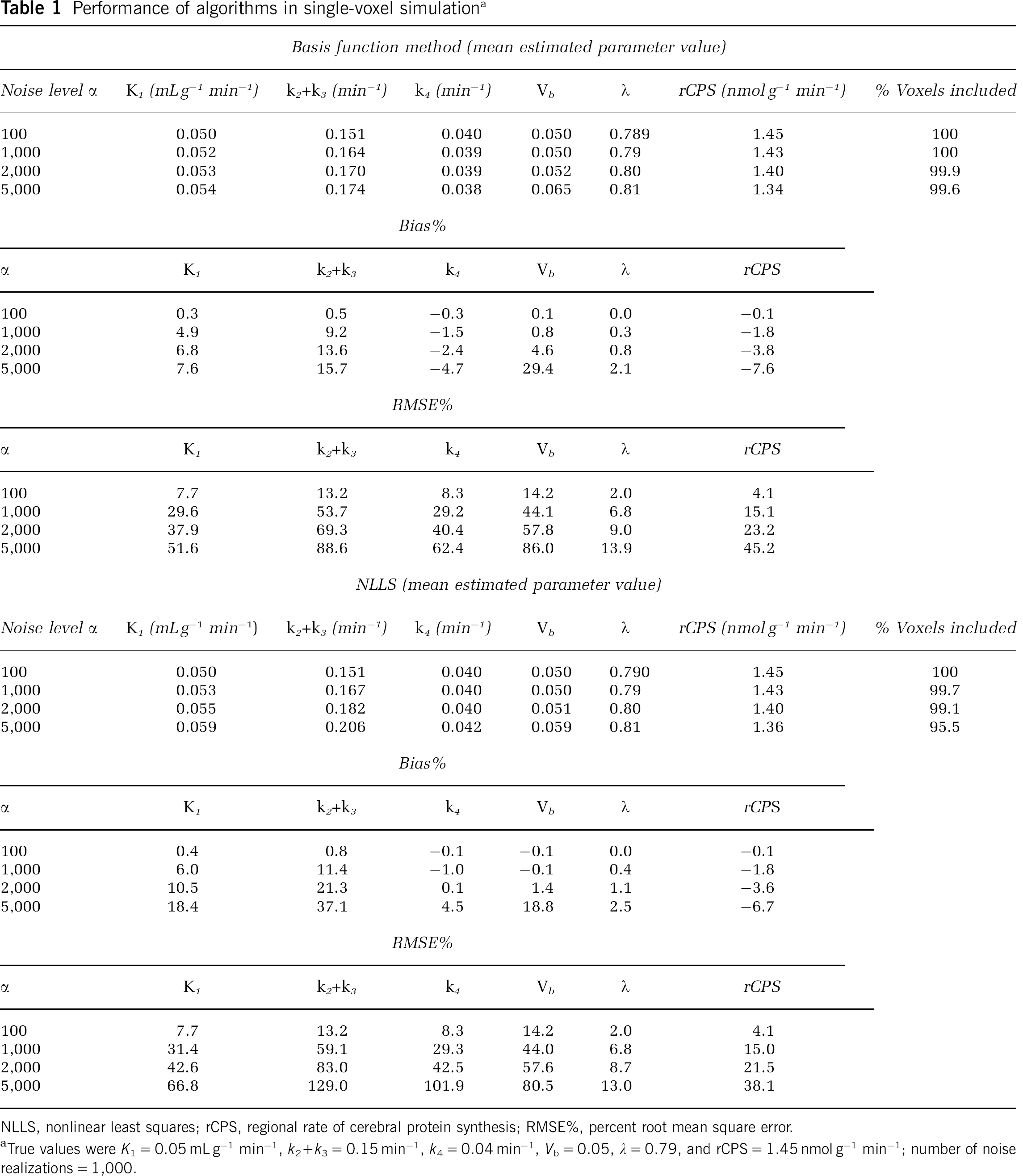
Results for single-voxel simulation are presented in Table 1. Basis function method performance was excellent at low noise levels (α = 100): bias in all parameter estimates was <1% in absolute value. At noise levels representative of those found in measured PET data (α = 1,000 to 2,000), biases in the estimates became non-negligible. In particular, K₁ and k₂ + k₃ were characterized by positive biases ranging from moderate (K₁) to severe (k₂ + k₃). k₄ was slightly underestimated, Λ was overestimated by < 1%, and rCPS was underestimated by <4%. Nonlinear least-squares performance was also excellent at low noise levels, but at higher noise levels, NLLS biases in K₁ and k₂ + k₃ were higher than with BFM, and k₄ was slightly overestimated. Nonlinear least squares biases in Λ and rCPS were comparable with those found with BFM. As expected, with both estimation methods, RMSE% increased as noise levels increased.

Table 1

Performance of algorithms in single-voxel simulation ^a

Basis function method (mean estimated parameter value)
Noise level α	K1 (mLg−1 min−1)	k 2 +k 3 (min−1)	k4 (min−4)	V b	Λ	rCPS (nmolg−1 min−1)	% Voxels included
100	0.050	0.151	0.040	0.050	0.789	1.45	100
1,000	0.052	0.164	0.039	0.050	0.79	1.43	100
2,000	0.053	0.170	0.039	0.052	0.80	1.40	99.9
5,000	0.054	0.174	0.038	0.065	0.81	1.34	99.6
Bias%
α	K 1	k 2 + k 3	k 4	V b	Λ	rCPS
100	0.3	0.5	−0.3	0.1	0.0	−0.1
1,000	4.9	9.2	−1.5	0.8	0.3	−1.8
2,000	6.8	13.6	−2.4	4.6	0.8	−3.8
5, 000	7.6	15.7	−4.7	29.4	2.1	−7.6
RMSE%
α	K 1	k 2 + k 3	k 4	V b	Λ	rCPS
100	7.7	13.2	8.3	14.2	2.0	4.1
1,000	29.6	53.7	29.2	44.1	6.8	15.1
2,000	37.9	69.3	40.4	57.8	9.0	23.2
5,000	51.6	88.6	62.4	86.0	13.9	45.2
NLLS (mean estimated parameter value)
Noise level α	K 1 (mLg−1 min−1)	k 2 +k 3 (min−1)	k 4 (min−1)	V b	Λ	rCPS (nmolg −1 min −1 )	% Voxels included
100	0.050	0.151	0.040	0.050	0.790	1.45	100
1,000	0.053	0.167	0.040	0.050	0.79	1.43	99.7
2,000	0.055	0.182	0.040	0.051	0.80	1.40	99.1
5,000	0.059	0.206	0.042	0.059	0.81	1.36	95.5
Bias%
α	K 2	k 2 + k 3	k 4	V b	Λ	rCPS
100	0.4	0.8	−0.1	−0.1	0.0	−0.1
1,000	6.0	11.4	−1.0	−0.1	0.4	−1.8
2,000	10.5	21.3	0.1	1.4	1.1	−3.6
5,000	18.4	37.1	4.5	18.8	2.5	−6.7
RMSE%
α>	K 1	k 2 + k 3	k 4	V b	Λ	rCPS
100	7.7	13.2	8.3	14.2	2.0	4.1
1,000	31.4	59.1	29.3	44.0	6.8	15.0
2,000	42.6	83.0	42.5	57.6	8.7	21.5
5,000	66.8	129.0	101.9	80.5	13.0	38.1

NLLS, nonlinear least squares; rCPS, regional rate of cerebral protein synthesis; RMSE%, percent root mean square error.

a

True values were K₁ = 0.05 mLg⁻¹ min⁻¹, k₂+k₃ = 0.15 min⁻¹, k₄ = 0.04 min⁻¹, V_b = 0.05, 1 = 0.79, and rCPS = 1.45 nmol g⁻¹ min⁻¹; number of noise realizations = 1, 000.

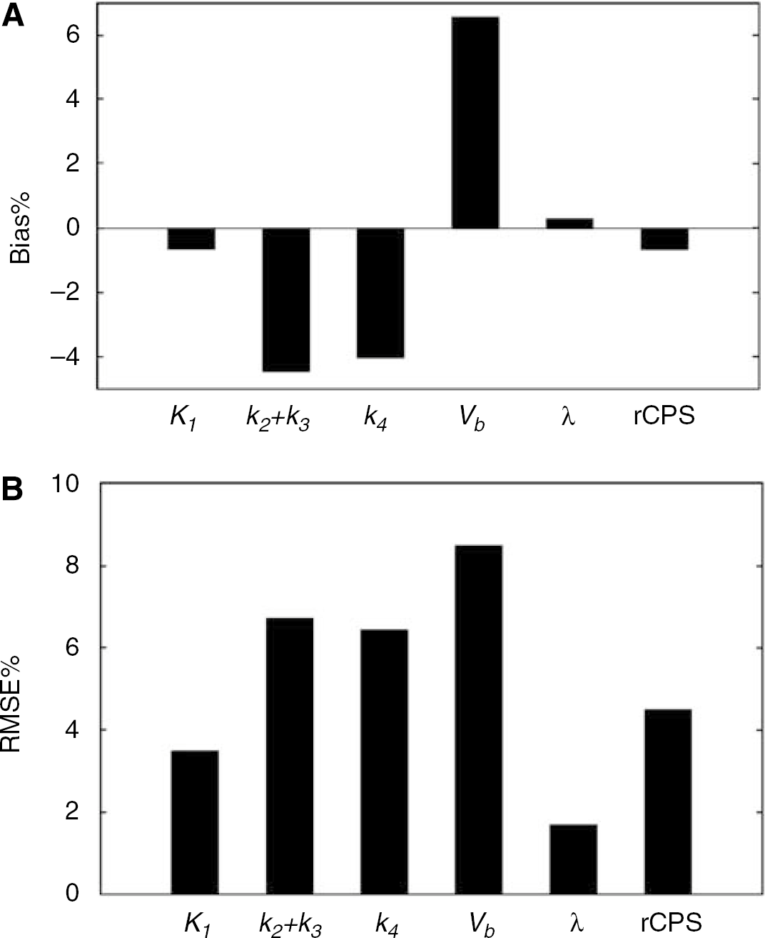
Comparisons between NLLS and BFM parameter estimates on a subset of voxels in the measured PET data are shown in Figure 2, in which NLLS estimates were taken as the ‘gold standard.’ Bias% and RMSE% of BFM estimates, relative to NLLS estimates, are shown. As noted earlier, comparisons exclude all voxels for which NLLS estimates of V_b or k₄ are < 10⁻⁴. Excluding these voxels, the total number of voxels analyzed in the two slices decreased by 9%, from 19, 468 to 17, 727. Biases of −4% were obtained for k₂ + k₃ and k₄, whereas K₁ showed almost no bias and lower RMSE%. Estimates of the most important parameters from a physiologic point of view, Λ and rCPS, had negligible biases (2 and 4.5%, respectively). As these comparisons assume that NLLS estimates represent true voxel parameter values, low biases in Λ and rCPS reflect agreement between estimation methods; they do not address whether both methods might have inherent biases.

Figure 2

Average Bias% (A) and RMSE% (B) of K₁, k₂ + k₃, k₄, V_b, Λ, and rCPS estimated using the basis function method. Parameters of the homogeneous tissue model were estimated for all voxels in one image plane from each of two subjects by both NLLS and BFM. Results were computed using Equations (9) and (10) with the NLLS estimate regarded as the true value. Only voxels with the NLLS estimates of k_b and V_b ≥ 10⁻⁴ were included in the statistics.

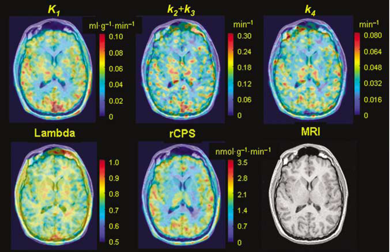
Parametric maps from the voxel BFM estimates of K₁ k₂ + k₃, k₄, Λ, and rCPS for one transverse slice from a [¹¹C]leucine PET study of a 23-year-old male are shown in Figure 3.

Figure 3

Parametric maps of K₁, k₂ + k₃, k₄, Λ, and rCPS obtained using the basis function method for one transverse image plane from a l[1-¹¹C]leucine PET study of an awake 23-year-old male subject. A Gaussian filter (FWHM 3.9 mm) was used to smooth each of the parametric images in three dimensions before visualization. The same image plane of the coregistered magnetic resonance image is shown in the bottom right.

Comparison of Voxel-Based and Region of Interest Time-Activity Curve-Based Analyses

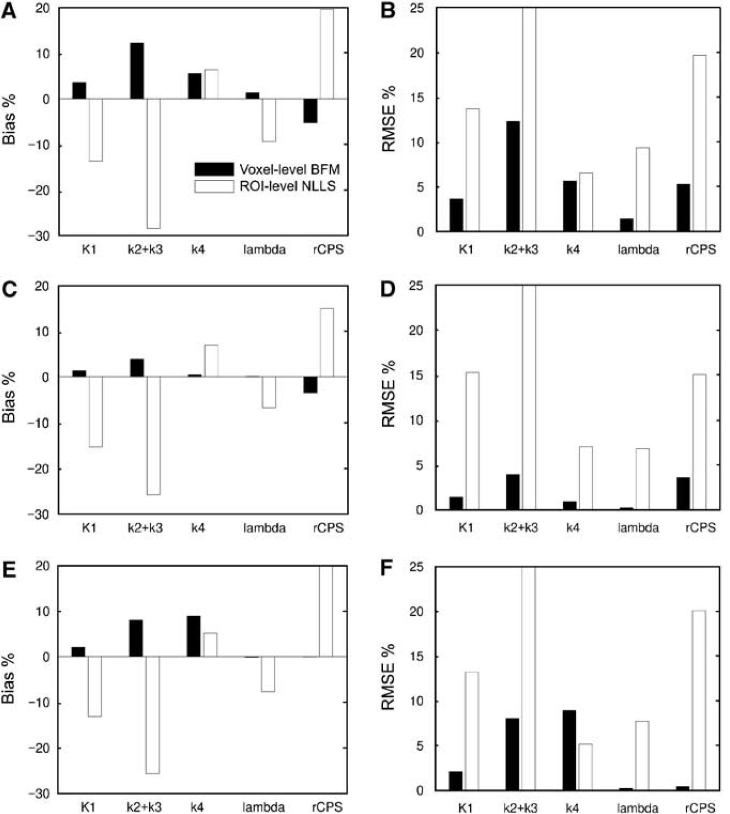
Bias% and RMSE% for multiple-voxel ROI simulations are shown in Figure 4. For each of the regions simulated (thalamus, corona radiata, and frontal cortex), the mean of the parameter values estimated in each voxel with BFM was compared with parameter estimates derived from the ROI TAC with NLLS. Results were quite consistent across ROIs in terms of direction and relative magnitude of biases. The voxel BFM method, consistent with single-voxel simulation, overestimated both K₁ and k₂ + k₃, but unlike single-voxel simulation, the estimates of k₄ were (on average) positively biased in the three regions. Regional means of voxel BFM estimates of Λ were excellent, but rCPS was underestimated by an average of 6, 4, and < 1% in the simulated frontal cortex, thalamus, and corona radiata, respectively. Performance of NLLS applied to the ROI TACs was worse. In particular, a substantial underestimation of k₂ + k₃ was found; this, together with a moderate overestimation of k₄, led to an underestimation of Λ by 6% to 10% and an overestimation of rCPS by 15% to 20%.

Figure 4

Bias% and RMSE% for multiple-voxel ROI simulation for central slices of the frontal cortex (A and B), thalamus (C and D), and corona radiata (E and F). Parameter estimates were computed in two ways: using basis function method (BFM) at the simulated voxel level and averaging the parameter estimates over all voxels within the ROI (voxel-level BFM), and using nonlinear least squares to fit the simulated ROI TAC (ROI-level NLLS). Bias% and RMSE% were computed by Equations (7) and (8) for each rate constant and each estimation method. See text for details.

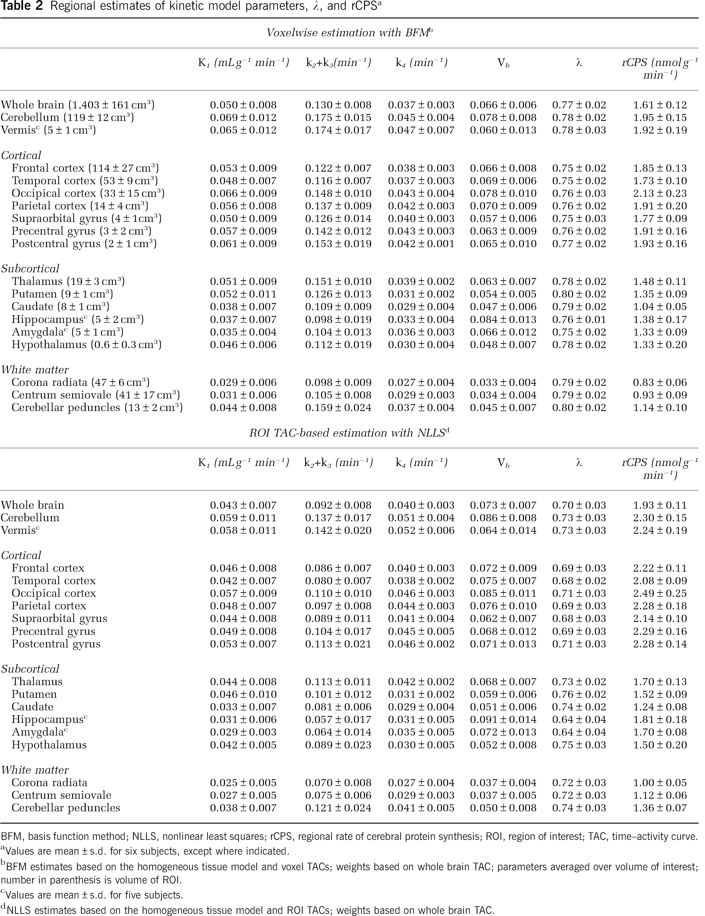
Table 2 compares the mean voxel BFM estimates with the estimates found by applying NLLS to the ROI TACs from measured PET data. The means and standard deviations for the six subjects are reported for 18 ROIs and whole brain. Consistent with simulation results, the estimates of K₁ were higher using the voxel BFM method than using NLLS applied to the ROI TACs. Estimates of k₂ + k₃ were substantially lower, and those of k₄ slightly higher, with ROI-level NLLS than with voxel BFM. Again, consistent with simulation, Λ estimates were ~5% to 10% lower and rCPS estimates were ~20% higher with ROI-level NLLS than with voxel BFM.

Table 2

Regional estimates of kinetic model parameters, Λ, and rCPS ^a

Voxelwise estimation with BFM b
	K1 (mLg -1 min -1 )	k2+k3(min -1 )	k4 (min -1 )	V b	Λ	rCPS (nmolg -1 min -1 )
Whole brain (1,403 ± 161 cm3)	0.050 ± 0.008	0.130 ± 0.008	0.037 ± 0.003	0.066 ± 0.006	0.77 ± 0.02	1.61 ± 0.12
Cerebellum (119 ± 12 cm3)	0.069 ± 0.012	0.175 ± 0.015	0.045 ± 0.004	0.078 ± 0.008	0.78 ± 0.02	1.95 ± 0.15
Vermis c (5 ± 1 cm3)	0.065 ± 0.012	0.174 ± 0.017	0.047 ± 0.007	0.060 ± 0.013	0.78 ± 0.03	1.92 ± 0.19
Cortical
Frontal cortex (114 ± 27 cm3)	0.053 ± 0.009	0.122 ± 0.007	0.038 ± 0.003	0.066 ± 0.008	0.75 ± 0.02	1.85 ± 0.13
Temporal cortex (53 ± 9 cm3)	0.048 ± 0.007	0.116 ± 0.007	0.037 ± 0.003	0.069 ± 0.006	0.75 ± 0.02	1.73 ± 0.10
Occipical cortex (33 ± 15 cm3)	0.066 ± 0.009	0.148 ± 0.010	0.043 ± 0.004	0.078 ± 0.010	0.76 ± 0.03	2.13 ± 0.23
Parietal cortex (14 ± 4 cm3)	0.056 ± 0.008	0.137 ± 0.009	0.042 ± 0.003	0.070 ± 0.009	0.76 ± 0.02	1.91 ± 0.20
Supraorbital gyrus (4 ± 1 cm3)	0.050 ± 0.009	0.126 ± 0.014	0.040 ± 0.003	0.057 ± 0.006	0.75 ± 0.03	1.77 ± 0.09
Precentral gyrus (3 ± 2 cm3)	0.057 ± 0.009	0.142 ± 0.012	0.043 ± 0.003	0.063 ± 0.009	0.76 ± 0.02	1.91 ± 0.16
Postcentral gyrus (2 ± 1 cm3)	0.061 ± 0.009	0.153 ± 0.019	0.042 ± 0.001	0.065 ± 0.010	0.77 ± 0.02	1.93 ± 0.16
Subcortical
Thalamus (19 ± 3 cm3)	0.051 ± 0.009	0.151 ± 0.010	0.039 ± 0.002	0.063 ± 0.007	0.78 ± 0.02	1.48 ± 0.11
Putamen (9 ± 1 cm3)	0.052 ± 0.011	0.126 ± 0.013	0.031 ± 0.002	0.054 ± 0.005	0.80 ± 0.02	1.35 ± 0.09
Caudate (8 ± 1 cm3)	0.038 ± 0.007	0.109 ± 0.009	0.029 ± 0.004	0.047 ± 0.006	0.79 ± 0.02	1.04 ± 0.05
Hippocampus c (5 ± 2 cm3)	0.037 ± 0.007	0.098 ± 0.019	0.033 ± 0.004	0.084 ± 0.013	0.76 ± 0.01	1.38 ± 0.17
Amygdala c (5 ± 1 cm3)	0.035 ± 0.004	0.104 ± 0.013	0.036 ± 0.003	0.066 ± 0.012	0.75 ± 0.02	1.33 ± 0.09
Hypothalamus (0.6 ± 0.3 cm3)	0.046 ± 0.006	0.112 ± 0.019	0.030 ± 0.004	0.048 ± 0.007	0.78 ± 0.02	1.33 ± 0.20
White matter
Corona radiata (47 ± 6 cm3)	0.029 ± 0.006	0.098 ± 0.009	0.027 ± 0.004	0.033 ± 0.004	0.79 ± 0.02	0.83 ± 0.06
Centrum semiovale (41 ± 17 cm3)	0.031 ± 0.006	0.105 ± 0.008	0.029 ± 0.003	0.034 ± 0.004	0.79 ± 0.02	0.93 ± 0.09
Cerebellar peduncles (13 ± 2 cm3)	0.044 ± 0.008	0.159 ± 0.024	0.037 ± 0.004	0.045 ± 0.007	0.80 ± 0.02	1.14 ± 0.10
ROI TAC-based estimation with NLLS d
	K 1 (mLg -1 min -1 )	k2 + k3 (min -1 )	k4 (min -1 )	V b	Λ	rCPS (nmolg -1 min -1 )
Whole brain	0.043 ± 0.007	0.092 ± 0.008	0.040 ± 0.003	0.073 ± 0.007	0.70 ± 0.03	1.93 ± 0.11
Cerebellum	0.059 ± 0.011	0.137 ± 0.017	0.051 ± 0.004	0.086 ± 0.008	0.73 ± 0.03	2.30 ± 0.15
Vermis c	0.058 ± 0.011	0.142 ± 0.020	0.052 ± 0.006	0.064 ± 0.014	0.73 ± 0.03	2.24 ± 0.19
Cortical
Frontal cortex	0.046 ± 0.008	0.086 ± 0.007	0.040 ± 0.003	0.072 ± 0.009	0.69 ± 0.03	2.22 ± 0.11
Temporal cortex	0.042 ± 0.007	0.080 ± 0.007	0.038 ± 0.002	0.075 ± 0.007	0.68 ± 0.02	2.08 ± 0.09
Occipical cortex	0.057 ± 0.009	0.110 ± 0.010	0.046 ± 0.003	0.085 ± 0.011	0.71 ± 0.03	2.49 ± 0.25
Parietal cortex	0.048 ± 0.007	0.097 ± 0.008	0.044 ± 0.003	0.076 ± 0.010	0.69 ± 0.03	2.28 ± 0.18
Supraorbital gyrus	0.044 ± 0.008	0.089 ± 0.011	0.041 ± 0.004	0.062 ± 0.007	0.68 ± 0.03	2.14 ± 0.10
Precentral gyrus	0.049 ± 0.008	0.104 ± 0.017	0.045 ± 0.005	0.068 ± 0.012	0.69 ± 0.03	2.29 ± 0.16
Postcentral gyrus	0.053 ± 0.007	0.113 ± 0.021	0.046 ± 0.002	0.071 ± 0.013	0.71 ± 0.03	2.28 ± 0.14
Subcortical
Thalamus	0.044 ± 0.008	0.113 ± 0.011	0.042 ± 0.002	0.068 ± 0.007	0.73 ± 0.02	1.70 ± 0.13
Putamen	0.046 ± 0.010	0.101 ± 0.012	0.031 ± 0.002	0.059 ± 0.006	0.76 ± 0.02	1.52 ± 0.09
Caudate	0.033 ± 0.007	0.081 ± 0.006	0.029 ± 0.004	0.051 ± 0.006	0.74 ± 0.02	1.24 ± 0.08
Hippocampus c	0.031 ± 0.006	0.057 ± 0.017	0.031 ± 0.005	0.091 ± 0.014	0.64 ± 0.04	1.81 ± 0.18
Amygdala c	0.029 ± 0.003	0.064 ± 0.014	0.035 ± 0.005	0.072 ± 0.013	0.64 ± 0.04	1.70 ± 0.08
Hypothalamus	0.042 ± 0.005	0.089 ± 0.023	0.030 ± 0.005	0.052 ± 0.008	0.75 ± 0.03	1.50 ± 0.20
White matter
Corona radiata	0.025 ± 0.005	0.070 ± 0.008	0.027 ± 0.004	0.037 ± 0.004	0.72 ± 0.03	1.00 ± 0.05
Centrum semiovale	0.027 ± 0.005	0.075 ± 0.006	0.029 ± 0.003	0.037 ± 0.005	0.72 ± 0.03	1.12 ± 0.06
Cerebellar peduncles	0.038 ± 0.007	0.121 ± 0.024	0.041 ± 0.005	0.050 ± 0.008	0.74 ± 0.03	1.36 ± 0.07

BFM, basis function method; NLLS, nonlinear least squares; rCPS, regional rate of cerebral protein synthesis; ROI, region of interest; TAC, time-activity curve.

a

Values are mean ± s.d. for six subjects, except where indicated.

b

BFM estimates based on the homogeneous tissue model and voxel TACs; weights based on whole brain TAC; parameters averaged over volume of interest; number in parenthesis is volume of ROI.

c

Values are mean ± s.d. for five subjects.

d

NLLS estimates based on the homogeneous tissue model and ROI TACs; weights based on whole brain TAC.

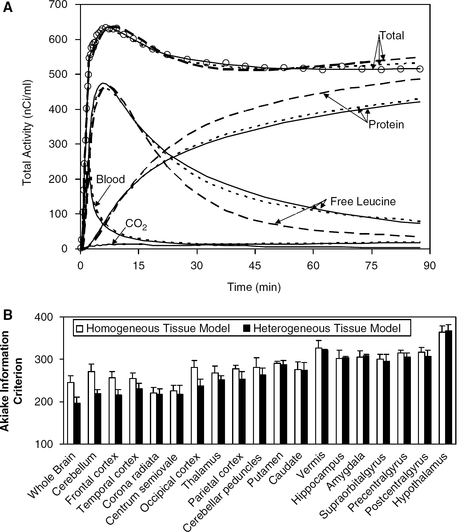
Figure 5A illustrates the NLLS fit of a cortical ROI TAC measured in one subject. The predicted time courses of labeled protein and free leucine in tissue, derived from estimated parameters, are also represented. ROI-level NLLS clearly overestimates measured activity in early and late frames of data and underestimates it in the intermediate interval. Figure 5A also shows the average of the TACs determined in each voxel, calculated from BFM parameter estimates for that voxel. The slower clearance of labeled leucine from the tissue and the slower accumulation of labeled protein estimated using voxel BFM are consistent with its lower rCPS determinations. Note that the average of the BFM voxel TACs fits more closely the measured data, but it still shows some systematic underestimation at intermediate times and overestimation in the late frames of data. This is evidence that this kinetic model for leucine is not fully adequate to describe ROI TACs and at least some voxel TACs. The assumption of tissue homogeneity, in particular, is not always a good approximation for a given region. The rates of blood flow, transport, metabolism, and incorporation of amino acids into protein vary regionally throughout the brain; the rates in gray and white matter are particularly different. Owing to the limited spatial resolution of even the HRRT (~ 2.6 mm FWHM), thinness of cortical areas (~3 to 5 mm), and white matter tracts that run through the subcortical gray matter, it is likely that activity measured in most ROIs, and possibly also in many voxels, derives from a heterogeneous mixture of tissues. For comparison, therefore, we illustrate activities estimated by fitting the ROI TAC using a kinetic model that specifically takes tissue heterogeneity into account; this model assumes that each tissue is composed of two homogeneous subregions, for example, gray and white matter (for model details, see Supplementary File). The fit provided by the tissue heterogeneity model is excellent, and activities in the free leucine and protein pools in the brain more closely resemble those found with voxel BFM than those derived by fitting the ROI TAC using the homogeneous tissue kinetic model for leucine.

Figure 5

Kinetic model fits of whole brain and regions of interest. (A) Open circles indicate activity measured in the frontal cortex of one subject, dashed lines represent activities estimated by fitting the ROI TAC using the homogeneous tissue kinetic model for leucine, and solid lines represent activities estimated by fitting the ROI TAC using a model that explicitly takes tissue heterogeneity into account. For comparison, the average of the TACs determined in each voxel from the BFM parameter estimates for that voxel are shown (dotted line). The predicted time courses of labeled protein and of free leucine in tissue, derived from the estimated parameters, are also represented. The predicted time courses of activity in blood within the ROI volume were approximately equal for all three methods. Tissue ¹¹CO₂ (bottom solid line) was very low throughout the study (< 15 nCi/mL). Note the substantially better fit of the heterogeneity model and the remarkable differences between the homogeneity and heterogeneity models applied to the ROI TACs in the predicted time courses of free [¹¹C]leucine and labeled protein in tissue. The average of the voxel BFM-estimated time courses of free [¹¹C]leucine and labeled protein resemble most closely those determined from the ROI TAC using the tissue heterogeneity model. Total activity predicted voxelwise using BFM was intermediate between the ROI-level homogeneity and heterogeneity model values; both voxel BFM and ROI-level homogeneity model NLLS overestimated the measured data at late times. Kinetic model fits showed similar patterns in all but the smallest and noisiest regions. (B) Goodness of fit, as measured by the Akaike Information Criterion (AIC), in whole brain and 18 ROIs. Values, computed by Equation (11) and averaged over six subjects, are displayed for the homogeneous tissue model (p = 4; white bars) and for the heterogeneous tissue model (p = 6; black bars) fits of the ROI TACs; ROIs are sorted in order of decreasing size. Error bars indicate standard deviation among subjects. Lower AIC values indicate better fits. A clear trend is visible with the tissue heterogeneity model yielding much lower mean AIC values for the largest ROIs; this indicates substantial improvements in fit over the homogeneous tissue model.

To further investigate the poor fits of the ROI TACs using the homogeneous tissue kinetic model, all ROI TACs were fitted with the kinetic model that explicitly takes tissue heterogeneity into account. Figure 5B shows the goodness of fit of ROI TACs by the two kinetic models for 18 ROIs and the whole brain. Akaike Information Criterion values, averaged over six subjects, are shown with ROIs sorted in order of decreasing size. In the whole brain, cerebellum, and the largest cortical ROIs, one secs the greatest improvement in fit by the use of a model that explicitly takes tissue heterogeneity into account, as indicated by much lower AIC values. In white matter and smaller ROIs, the two models produced more similar AIC values. Estimates of rCPS based on applying the tissue heterogeneity model to ROI TACs, however, were considerably more variable than those produced either by voxelwise BFM estimation or by fitting the homogeneous tissue model to the ROI TACs (data not shown). Furthermore, the heterogeneity model estimation did not always converge, probably because of the presence of six parameters in the model. For these reasons, the tissue heterogeneity model was not pursued further as a practical alternative for estimation of rCPS.

Discussion

Prior to this study, estimation of kinetic model parameters of the l-[1-¹¹C]leucine PET method has been carried out only at the ROI level. In this study, we addressed our attention to the generation of parametric maps. Such maps provide important information regarding heterogeneity within a region and take full advantage of the high spatial resolution of the scanner for visualization of parameters. Our purpose was not to compare subjects at the voxel level; this type of analysis would require spatial normalization with its inherent uncertainties about the actual anatomical location of a voxel. Rather, we are using a voxel-based estimation method to compute the mean estimates of parameters for an anatomically defined ROI. A voxel-based estimation method applied to high-spatial-resolution images may mitigate some of the problems of tissue heterogeneity inherent in PET data.

As the cost of standard NLLS estimation at the voxel level is prohibitive, BFM was used as a computationally feasible alternative. The time required for the analysis of one image plane decreased from ~ 2 h using NLLS to ~ 1 min using BFM. Further savings in computational time could be achieved if estimation were carried out first on a coarse grid of βs and then on a finer one, as proposed by Koeppe et al (1985). In a subset of measured voxels from two PET studies, BFM yielded estimates in very good agreement with NLLS estimates. In single-voxel simulation, BFM provided excellent performance at low noise levels, but at higher noise levels, including those typical of measured voxel data, the method was characterized by high RMSE% and non-negligible positive biases that were moderate for K₁ and much higher for k₂ + k₃. The most important parameters from a physiologic point of view, Λ and rCPS, were only slightly biased, except at the very highest voxel noise levels. Simulation results and the good agreement between BFM and NLLS suggest that, in this case, it is the high noise level inherent in voxel data, rather than our choice of algorithm, that is responsible for observed biases. We are currently investigating whether improvements in performance can be achieved by pre-processing data to reduce the noise of voxel TACs.

One remarkable outcome of the analysis was the poor performance of the homogeneous tissue kinetic model for leucine when applied to ROI TACs. Simulations showed a substantial underestimation of k₂ + k₃ (−20% to −30%), which, along with a moderate overestimation of k₄, led to the underestimation of Λ by ~8% and the overestimation of rCPS by as much as 15% to 20%. Differences of a similar magnitude were observed in measured data between ROI-level homogeneous tissue model estimates and mean voxel-level BFM estimates. In addition, fits of the homogeneous tissue model to ROI TACs were generally poor: in 73% of ROIs examined in six subjects, AIC showed that a kinetic model that explicitly takes tissue heterogeneity into account provided the better fit. This strongly suggests the need for a model that takes tissue heterogeneity into account for analysis of l-[1-¹¹C]leucine at the ROI level.

The effects of tissue heterogeneity have been investigated earlier for [¹⁴C]deoxyglucose and [¹⁸F]fluorodeoxyglucose (Schmidt et al, 1991, 1992, 1995). From the similarities between the model for deoxyglucose/fluorodeoxyglucose and the model for leucine, overestimation of k₂ + k₃ and k₄ was predicted if a model that assumes tissue homogeneity is used. In this study, k₄ was somewhat overestimated under these conditions, but k₂ + k₃ was substantially underestimated, contrary to expectation. To overcome limitations of the homogeneous tissue model, we evaluated a heterogeneous tissue model comprising two subregions for each ROI. The heterogeneity model fit ROI TACs extremely well. For estimating parameters, however, it performed poorly on measured PET data. It is our view that more work is required to develop a useful tissue heterogeneity model for analysis of ROI TACs, or alternative approaches that do not require homogeneity assumptions are required.

We did not apply the heterogeneity model at the voxel level because of the high number of parameters to be estimated. With voxel BFM, we did observe some systematic misfit of data: measured total activity was underestimated at intermediate times and overestimated at later times. The direction of the systematic overestimation/underestimation was similar to that found when the ROI TAC was fitted with the tissue homogeneity model, but the magnitude of the disparity was less with voxel BFM. This suggests that the homogeneous tissue model may not be fully adequate for at least some voxels. These errors in model specification will be reflected in errors in parameter estimates. Furthermore, measurement noise interacts with model specification error in affecting final parameter estimates. Other scanners have different noise properties, and those with lower spatial resolution may be more affected by tissue heterogeneity; hence, voxel parameter estimates may show different bias and RMSE from that found in this study.

Differences in parameter values estimated with different procedures are not unique to l-[1-¹¹C]leucine studies. Each of the factors examined in this study (choice of model to define relationships among parameters, noise level in the data, algorithm used for parameter estimation) affects the estimates. It has long been recognized that using different kinetic models gives rise to differences in both micro- and macroparameter estimates that can be substantial, even when each model is applied to the same TAC (Lammertsma et al, 1987). Ultimately, all models oversimplify the underlying tissue kinetics and some degree of model specification error occurs. However, even in the absence of model specification error, estimation biases can occur because of measurement noise in the data or error in measurement noise characterization. Thus, we should expect differences between parameter estimates at the voxel level (potentially greater homogeneity and less model mis-specification, but higher noise levels) and at the ROI level (lower noise levels, but potentially more heterogeneity and model specification error). Yet, few studies have quantitatively compared parameter estimates at the voxel and ROI levels. In one such study, several methods for estimating binding potentials for dopamine and 5-HT_1A receptors were compared; even when the same analysis procedure was used, the estimates differed substantially between ROI-based and voxel-based methods (Cselényi et al, 2006). In this study, we also found substantial differences between ROI-based and voxel-based estimates of kinetic model parameters when the same homogeneous tissue model was used in both analyses. As each method has its own set of limitations, we used simulation to look at the bias and RMSE of each procedure under consideration. We also examined how the different methods compare when applied to measured data, taking into account each method's limitations.

Of the methods examined for determining kinetic model parameters for l-[1-¹¹C]leucine in identified ROIs, the voxel BFM method provided the best overall performance. This method requires an estimation of parameters, Λ, and rCPS for each voxel, and averaging of values over all voxels within the region. Simulations suggest that resultant biases in Λ and rCPS are small. Furthermore, intersubject variability of parameters estimated using voxel BFM in measured PET data was low, comparable with that achieved by the ROI-based application of the homogeneous tissue model. Minimally biased, low variance estimates are important for tracking changes in rCPS and/or Λ across regions and over time, particularly as changes may be relatively small in magnitude. Optimal estimates will also be required for rCPS to be used as an objective means by which to identify abnormalities or as an outcome measure to evaluate potential treatments. Ultimately, these quantitative measurements in human subjects may give new insights into mechanisms underlying pathologies in neurodevelopmental, cognitive, and neurodegenerative disorders. Basis function method analysis of l-[1-¹¹C]leucine data at the voxel level is a useful tool for the quantitative determination of rCPS.