
Abstract
This article investigates the relation between stimulus-evoked neural activity and cerebral hemodynamics. Specifically, the hypothesis is tested that hemodynamic responses can be modeled as a linear convolution of experimentally obtained measures of neural activity with a suitable hemodynamic impulse response function. To obtain a range of neural and hemodynamic responses, rat whisker pad was stimulated using brief (≤2 seconds) electrical stimuli consisting of single pulses (0.3 millisecond, 1.2 mA) combined both at different frequencies and in a paired-pulse design. Hemodynamic responses were measured using concurrent optical imaging spectroscopy and laser Doppler flowmetry, whereas neural responses were assessed through current source density analysis of multielectrode recordings from a single barrel. General linear modeling was used to deconvolve the hemodynamic impulse response to a single “neural event” from the hemodynamic and neural responses to stimulation. The model provided an excellent fit to the empirical data. The implications of these results for modeling schemes and for physiologic systems coupling neural and hemodynamic activity are discussed.
Keywords
The technique of blood oxygen level–dependent (BOLD) functional magnetic resonance imaging has become increasingly important for investigation of the functioning brain. Since the inception of the technique in the early 1990s (Kwong et al., 1992; Ogawa et al., 1992), much research has been undertaken into the relation between underlying hemodynamic changes and the BOLD signal source. As a result, the BOLD signal source is well characterized in terms of blood variables, and several quantitative biophysical models of the BOLD signal are available (Boxerman et al., 1995; Davis et al., 1998; Ogawa et al., 1993). Despite the successes of this research, however, the somewhat prior relation between underlying neural activity and hemodynamic changes is less clear. The research reported here aims to explain the neural–hemodynamic coupling in terms of a linear convolution of an experimentally obtained hemodynamic impulse response with experimentally obtained neural responses.
The anatomic and functional specialization of rat “barrel” cortex make it a system of choice for studying neural and hemodynamic responses to stimulation. Each whisker on the rat's face projects to a discrete area of contralateral somatosensory cortex (a “barrel”) that has its own local blood supply and that responds most strongly to a single principal whisker (Patel, 1983; Welker, 1976; Woolsey and Van der Loos, 1970). The system is therefore easy to stimulate in a controlled way. Furthermore, the superficial location of rat cortex enables simultaneous intrinsic optical imaging and spectroscopy, and laser Doppler flowmetry (Jones et al., 2001). The laminar organization, coupled with synchronous activation of apically orientated intrinsic neurons, makes the system ideal for one-dimensional current source density analysis of spatially distributed evoked field potentials.
A recent study by Logothetis et al. (2001) found that, although there was a good correlation between multiunit activity and BOLD response, summed evoked field potential (EFP) recordings were significantly better than either single- or multiunit recordings at predicting the BOLD response in visual cortex. Furthermore, other studies have found the peak hemodynamic response to be a linear function of summed EFP amplitude (Mathiesen et al., 1998; Ngai et al., 1999) (also Sheth et al., 2003, in press). Various anatomic and physical arguments lead to the conclusion that the main contribution to extracellular EFPs comes from excitatory postsynaptic potentials (EPSPs) (Mitzdorf, 1985). Therefore, peak hemodynamic activity is likely to reflect the excitatory synaptic input, rather than the efferent activity, of a neural population (see also Discussion).
As a consequence of the principle of superposition, the EFPs generated by current sinks and sources add algebraically at any given point, making interpretation of EFP signals ambiguous. The technique of current source density (CSD) analysis allows the transformation of laminar recordings of EFPs into spatially distinct current sinks and sources, where sinks correspond to dendritic EPSPs and sources correspond to passive efflux of charge from nerve cell bodies (Mitzdorf, 1985; Nakagawa and Matsumoto, 2000; Nicholson and Freeman, 1975). The resultant disambiguated current sink/source measurements facilitate both interpretation of the data and comparison of the data across animals. Collection of EFP data for CSD analysis has traditionally been performed sequentially, but recent improvements in probe design have enabled many channels of data to be acquired simultaneously, allowing much greater flexibility in experimental design. The present study used CSD analysis of laminar EFP recordings, and the resultant measure of “neural activity” is defined as current sink amplitude in response to a stimulus.
To assess the corresponding hemodynamic response to stimulation, the combined techniques of intrinsic optical imaging spectroscopy (OIS) and laser Doppler flowmetry (LDF) are used. Optical imaging spectroscopy explains the reflectance spectra of a region of tissue in terms of textbook spectra for oxy- and deoxyhemoglobin (HbO2 and Hbr, respectively). Given certain assumptions about baseline values, OIS can provide quantitative estimates of fractional changes in total hemoglobin concentration and saturation levels. Under the assumption of a relatively constant hematocrit level (Kleinfeld et al., 1998), changes in total hemoglobin concentration can be further interpreted in terms of blood volume changes. Laser Doppler flowmetry provides a measure of relative changes in blood flow by calculating the Doppler shift imparted to remitted illumination by moving red blood cells. Combined LDF and OIS measurements therefore provide estimates of fractional changes in oxy- and deoxyhemoglobin, blood volume, and blood flow.
To obtain a range of neural and hemodynamic responses, we chose to use two experimental paradigms: one in which paired pulses were applied with a separation in the range 100 to 1,000 milliseconds; and the other in which stimuli of constant duration (2 seconds) but varying frequency (1 to 5 Hz) were applied. Brief stimuli (≤2 seconds) were used to avoid confounding effects of neural adaptation to prolonged stimuli (see also Discussion). A “neural event” is defined as the current sink response to a single electrical stimulus pulse (0.3 millisecond, 1.2 mA), whereas the neural response to a stimulus may consist of up to 10 (2 s, 5 Hz) “neural events.” The neural response to the second of the paired pulses is known to be inhibited up to a separation of ≈600 milliseconds during forepaw stimulation, and a recent study has shown this to be reflected in the resultant BOLD response (Ogawa et al., 2000). For stimuli of different frequencies, all but the first neural response are found to be inhibited in a frequency-dependent manner and thus the mean neural response decreases with increasing stimulation frequency. As mentioned previously, the summed neural activity (in terms of summed EFP amplitudes) has been found to be linearly related to peak hemodynamic changes. We used two stimulation paradigms to enable independent (and hopefully convergent) estimates of hemodynamic impulse responses. The characteristics of the neural system(s) underlying the observed response inhibition are not explicitly addressed in this paper.
MATERIALS AND METHODS
Animal preparation
Female hooded Lister rats weighing between 250 and 400 g were kept in a 12-h dark/light cycle environment at a temperature of 22°C with food and water ad libitum. Before surgery, animals were anesthetized with urethane (1.25 g/kg intraperitoneally) with additional doses of urethane (0.1 mL) administered if necessary. Atropine was also administered (0.24 mg/kg subcutaneously) to reduce mucous secretions during surgery. Rectal temperature was maintained at 37°C throughout surgical and experimental procedures using a homeothermic blanket (Harvard Apparatus, Holliston, MA, U.S.A.). Animals were tracheotomized to allow artificial ventilation and measurement of end-tidal CO2. The femoral vein and artery were cannulated to allow drug infusion and measurement of mean arterial blood pressure, respectively. Animals were placed in a stereotaxic frame (Kopf Instruments, Tujunga, CA, U.S.A.). Before OIS, the skull overlying the somatosensory cortex was thinned to translucency with a dental drill under constant cooling with saline. A plastic “well” was attached to the thinned skull and filled with saline (37°C) to reduce specularities from the skull surface. After OIS, the skull overlying somatosensory cortex was removed completely, and the dura overlying the chosen barrel area was removed. The multielectrode probe was then inserted normal to cortical surface under micromanipulator control. At the end of each experiment, animals were perfused for subsequent cytochrome oxidase histology. Physiologic parameters were continuously monitored and maintained in normal ranges. All procedures were carried out in accord with Home Office regulations.
Localization of activated region in barrel cortex for electrode placement
Somatosensory cortex was monochromatically illuminated (narrow bandwidth interference filter, ± 5 nm) and images were recorded using a 12-bit CCD camera (SMD 1M60). Barrel cortex was first located by electrically stimulating the entire whisker pad (5 Hz, 1 second, 1.2 mA). Thirty trials were collected at 15 Hz, each of 12-second duration, stimulus onset at 8 seconds, 15-second interstimulus interval. Images were analyzed using a weak model algorithm (Molgedey and Schuster, 1994) as previously described (Zheng et al., 2001). The same paradigm was then used with mechanical stimulation (5 Hz, 1 second) of a single whisker (central location, such as C2), to reveal the location of a single barrel field. The single barrel maps were registered with images of cortical surface to guide insertion of the electrophysiology probe.
Optical spectroscopy and laser Doppler flowmetry
Concurrent LDF and OIS were performed as described previously (Jones et al., 2001) and are only briefly outlined here. After localization of barrel cortex, a spectrographic slit and an LDF probe (PeriFlux 5010; Perimed, Stockholm, Sweden, 780-nm illumination, 0.25-mm separation) were placed over the area of interest. Visual inspection of cortical surface through the translucent thinned skull preparation allowed large vessels to be avoided during both spectrographic slit and LDF probe placement. Cortex was illuminated with visible light and data were collected in the wavelength range 500 to 640 nm. To prevent crosstalk between the two modalities, appropriate filters were used. Spectroscopic data were analyzed using a path-length scaling algorithm (Mayhew et al., 1998). The signal from the LDF probe was analyzed by an LDF spectrometer, which includes a proprietary linearization algorithm (Nilsson, 1984) to reduce errors caused by changes in blood volume. The LDF signal was then digitized continuously using a 1401plus (CED Ltd., Cambridge, U.K.). The time constant of the LDF recordings was 0.2 second, and the bandwidth was 12 kHz. Thirty trials were obtained for each stimulus condition, with a trial length of 23 seconds (stimulus onset at 8 seconds) and an interstimulus interval of 25 seconds (sufficient to avoid any hemodynamic refractory effects).
Electrophysiology
Electrophysiologic recordings were made using a 16-electrode probe (100 μm spacing; CNCT, University of Michigan) coupled to a data acquisition device (Medusa Bioamp; Tucker-Davis Technologies, Alachua, FL, U.S.A.) with a custom-written Matlab (The Mathworks Inc., Natick, MA, U.S.A.) interface. The probe was advanced under visual (through a microscope) and audio (lowermost channel signal connected to amplifier) monitoring until just touching cortex at the activated region identified by the optical techniques described above. The probe was then inserted normal to cortex to a depth of 1,500 μm (uppermost electrode at cortical surface). Recordings were averaged over 60 trials for each stimulus condition, with stimulus onset “jittered” within a 20-millisecond window to reduce effects of 50-Hz mains noise. The resultant evoked field potential recordings were sampled at 6 kHz with 16-bit resolution.
Given the assumption that the conductivity tensor σ is constant (homogeneity) and that field potentials φ vary only along a single dimension (anisotropy), the following one-dimensional CSD equation can be used:
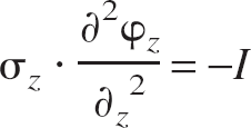
where z is the axis of measurement and I = current source distribution (time dependence of φ and I omitted for clarity). The assumption of anisotropy is valid in rat whisker barrel because large sheets of apically oriented neurons fire synchronously (Di et al., 1990). The assumption of homogeneity is an acceptable one and may introduce less error than incorrect estimation of the conductivity tensor (Rappelsberger et al., 1981).
To perform CSD analysis on the recorded field potentials, we used the method of Rappelsberger et al. (1981). First, the spatial resolution of the data was increased by interpolation using local (four points) third-order polynomial estimates. A finite difference formula was then applied to obtain the second spatial differential. Finally, a Hamming window was applied to alleviate any high-frequency noise introduced by the interpolation scheme. The final two steps can be applied simultaneously using the equation
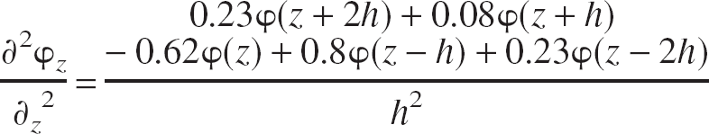
where h = distance between data points (50 μm after interpolation). This analysis was performed for each time point. The resultant data were compared with the second difference of the original raw data in every case to ensure that only the resolution and noise of the data had been altered, rather than the spatio-temporal characteristics of the activation patterns.
Stimulus presentation and paradigms
All stimulus presentation was controlled through a 1401plus (CED Ltd.) running custom-written code with stimulus onset time locked to the CCD camera or the electrophysiology recording unit. Electrical stimulation of the whole whisker pad was delivered via tungsten electrodes inserted in an anterior direction each side of the whisker pad. All electrical stimuli were presented at 1.2 mA with a 0.3-millisecond individual pulse width: a robust but nonnoxious stimulus (Jones et al., 2001). Mechanical stimuli were presented by a hypodermic needle attached to an electrical relay that moved a single whisker ≈2 mm in the rostrocaudal axis. For the frequency modulation protocol, 2-second stimuli of 1, 2, 3, 4, and 5 Hz were applied. For the paired pulse experiments, a stimulus consisted of two pulses with a separation ranging from 100 to 1,000 milliseconds in steps of 100 milliseconds. Stimuli were randomly interleaved within a single experimental run and were presented with an interstimulus interval of either 25 seconds (hemodynamic) or 6 seconds (electrophysiology).
Data preparation and normalization
The CSD analysis process results in time series of responses at each cortical depth. Because the spatial pattern of activation did not change with stimulation paradigm, the first principal component (accounting for >80% of the data in every data set) was used to collapse the data across the spatial dimension. The CSD time series response to the first pulse of each stimulus was then normalized to have unity depth (Figs. 1C and 1D), and the normalized magnitudes of the individual pulse responses used for interanimal averaging. The absolute amplitudes of the first individual pulse responses showed no significant differences within animals across stimulus conditions, indicating that the same effective normalization factor was used within each animal's neural data.
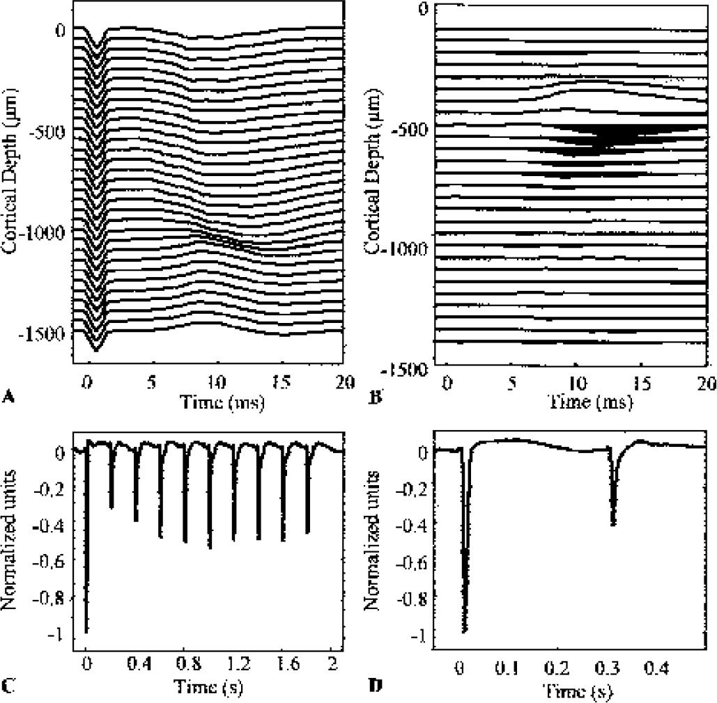
Representative electrophysiology data.
To reduce the substantial interanimal variation in hemodynamic response magnitude, all data were normalized before interanimal averaging. For clarity, only blood flow and volume changes are displayed in this report, although the results hold for oxygenated and deoxygenated hemoglobin signals also. Paired pulse data were normalized such that the magnitude of the 1-second separation response was unity, whereas the frequency data were normalized such that the 2-second, 1-Hz response magnitude was equal to unity. These normalization conditions are equivalent, allowing for direct comparisons between the data sets from the two experimental paradigms.
RESULTS
Response characteristics
The multichannel electrophysiology recordings revealed the time-varying EFP signals across the layers of a single whisker barrel in response to a single stimulus pulse (Fig. 1A). Note the polarity inversion approximately 500 μm below the cortical surface. Subsequent CSD analysis (Fig. 1B) revealed a large current sink at this level. This current sink corresponds to the primary excitatory input from the thalamus, which is known to terminate in layer IV (Armstrong-James et al., 1992). The normalized first principal component (see Materials and Methods) of the neural response revealed clear inhibition effects (Figs. 1C and 1D). The neural response to a frequency stimulation showed immediate inhibition followed by return to a steady state. The amplitude of this steady state was frequency dependent. The second of the paired-pulse responses showed separation-dependent inhibition.
In contrast to the resolvable single stimulus pulse responses seen in the electrophysiology data, the long time constant of hemodynamic effects ensured that only a single hemodynamic response was observed in response to a 2-second train of stimulus pulses (Fig. 2A). The blood flow response peaked earliest at ≈2.5 seconds, with volume and oxyhemoglobin peaking at ≈3 seconds. Blood flow changes increased monotonically with stimulation frequency (Fig. 2B).
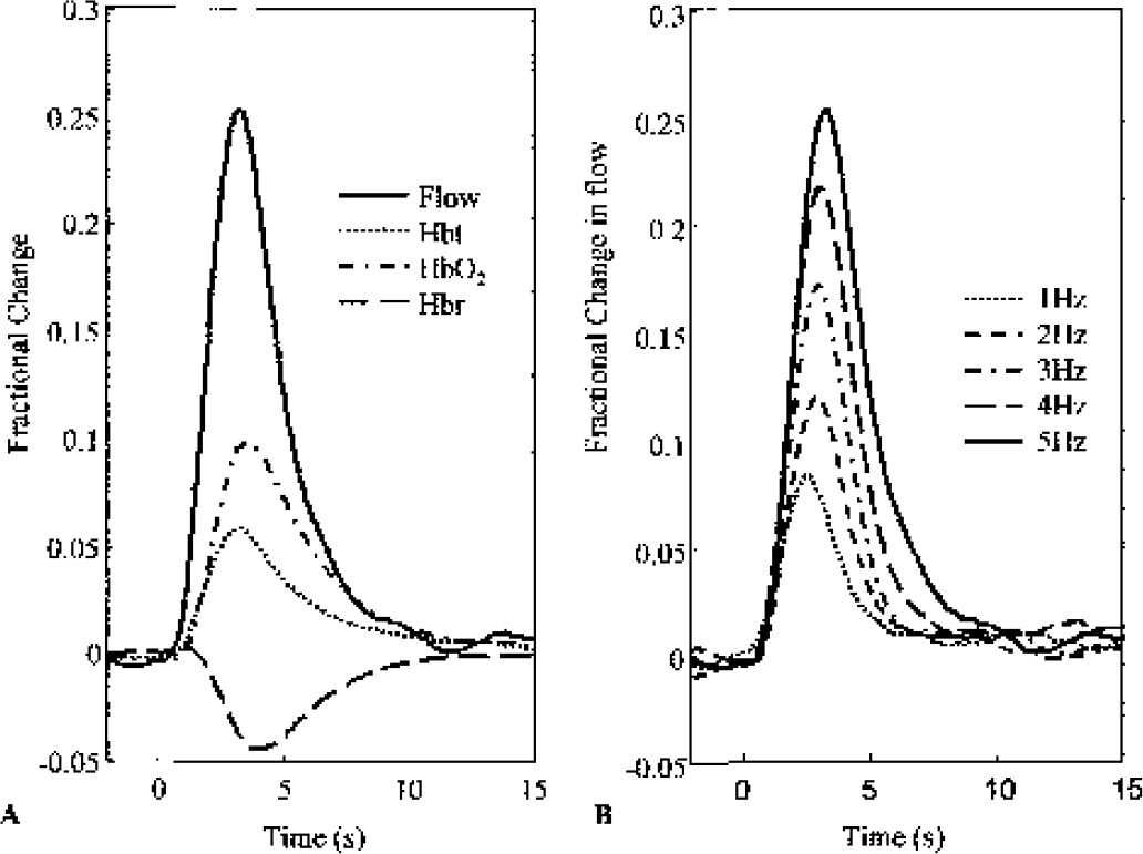
Sample hemodynamic data.
Response modulation
The absolute magnitudes of the normalized single pulse responses were used to form either a mean or summed “neural activity” statistic. The peak magnitude of the normalized hemodynamic changes was used to quantify hemodynamic responses to stimulation. As stimulation frequency increased, mean neural activity monotonically decreased (Fig. 3A), whereas summed neural activity, blood flow changes, and blood volume changes all increased monotonically (Figs. 3B–D). Blood flow and blood volume changes were found to be linear with summed neural activity (Figs. 3E and 3F), as summarized by

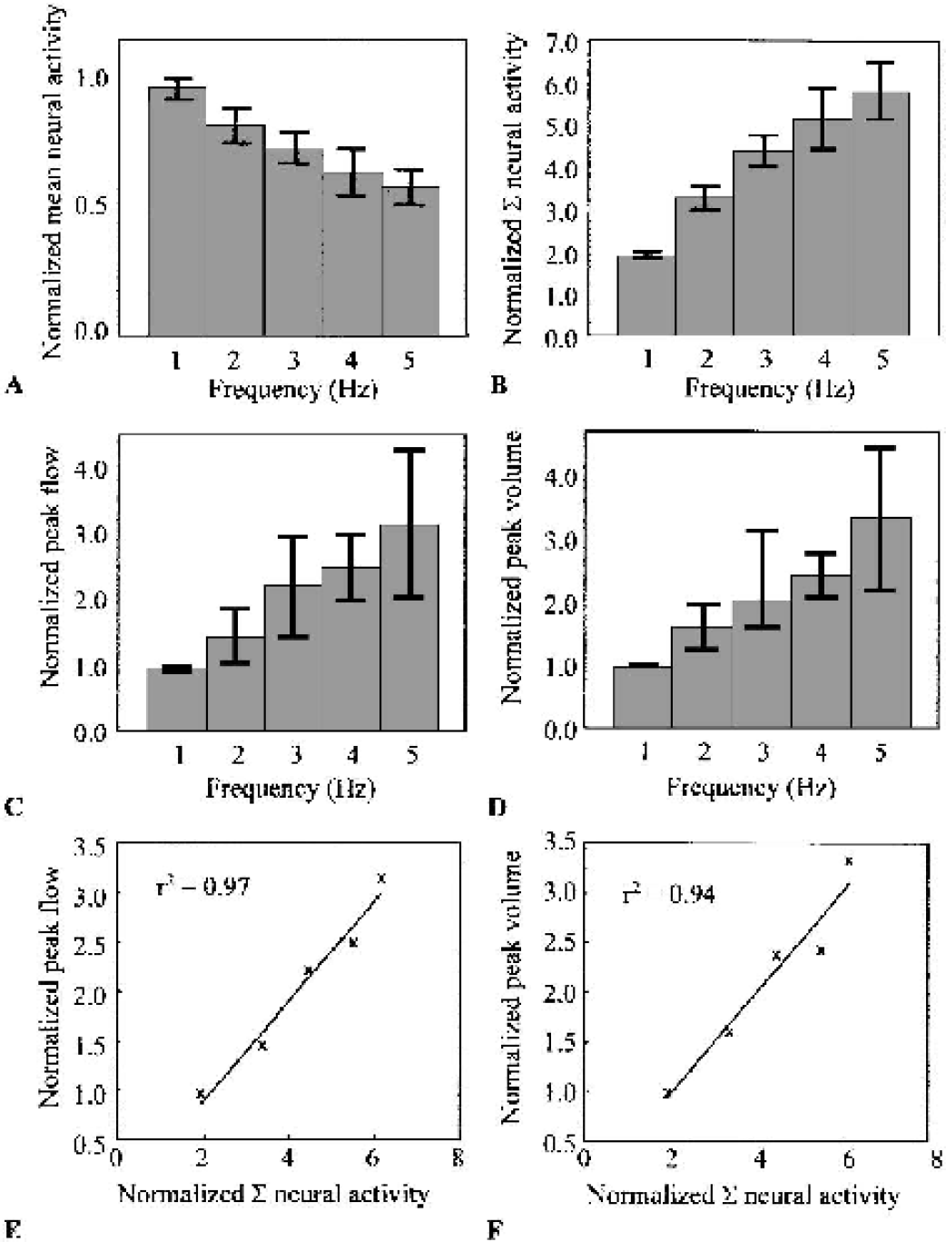
Peak hemodynamic changes are a linear function of summed neural activity (Σ) for frequency-dependent responses (n = 6).
This relation is consistent with previously reported data (Mathiesen et al., 1998; Ngai et al., 1999).
The neural response to the second of the paired pulses was inhibited strongly at 100 milliseconds and only recovered completely at ≈700 milliseconds (Fig. 4A—dashed line represents expected response magnitude in the absence of inhibition effects). These results are similar to those reported in Ogawa et al. (2000). However, peak hemodynamic changes did not follow the same pattern (Figs. 4B and 4C), and thus the relation described by Eq. 3 did not hold for the paired pulse data set (Figs. 4D and 4E), arguing against the application of such a simple linear model.
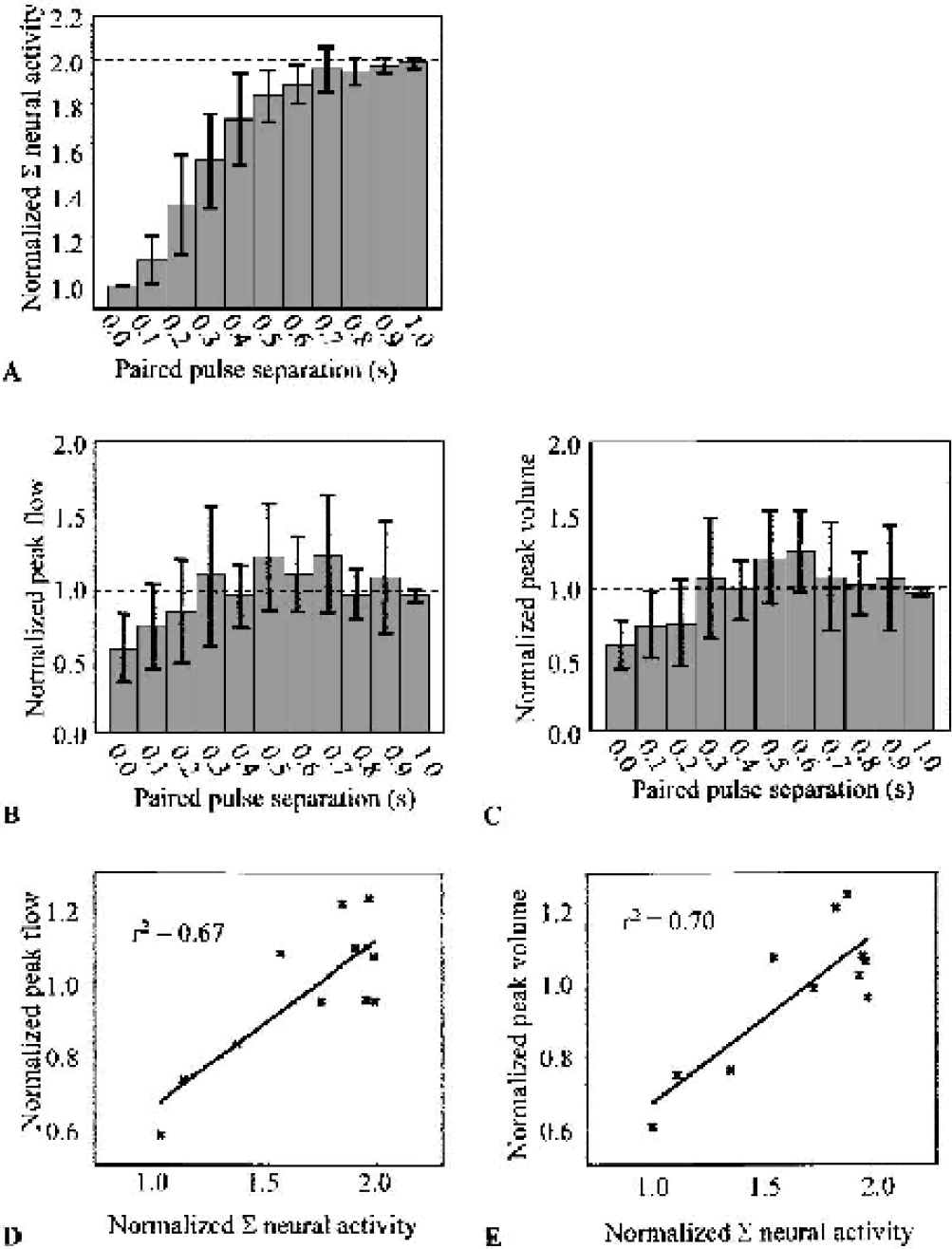
Peak hemodynamic changes are not a linear function of summed neural activity (Σ) for paired pulse responses (n = 7).
Impulse response estimation
The use of peak hemodynamic change as a representative statistic neglects much of the information in the hemodynamic response measurements. Instead, we tested the hypothesis that the hemodynamic responses can be modeled as a linear convolution of experimentally obtained neural event magnitudes with suitable hemodynamic impulse responses. To identify suitable hemodynamic impulse response estimates, we used general linear modeling (GLM), thus including all available data in the analysis.
General linear modeling analysis attempts to explain data in terms of a model weighted by parameters that are adjusted to minimize the residual least-squares errors (Fig. 5A). The model is specified in a design matrix. A common approach in functional magnetic resonance imaging data analysis is to specify a model in terms of several canonical response functions and then use GLM analysis to optimize the amplitudes of those functions. This approach vastly reduces the dimensionality of the GLM calculations—a critical consideration when dealing with data sets containing many thousands of pixels for each time point. However, because in the present case we obtained only a single time series from the active area, we used a weak model in which every clock tick of the response is represented by an individual parameter, thus ensuring that no particular response “shape” was specified a priori. Delta functions scaled by the normalized magnitudes of the experimentally derived neural events were input into the design matrix (Fig. 5B), which was defined at a clock rate of 60 Hz to ensure that all stimuli started on an integer clock tick. Sixteen independent data sets were available (5 different stimulus frequencies, 11 different paired pulse separations) to estimate impulse responses. A convergence of the estimates can be taken as evidence that the linear convolution model is appropriate.
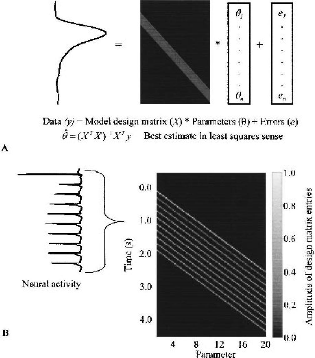
General linear modeling of impulse responses.
Results of the GLM analysis revealed a tight grouping of the individual impulse response estimates about the group means (Fig. 6). This convergence of the response estimates indicates that the use of a linear convolution model is appropriate. Because of the common normalization condition, the impulse response estimates for the frequency and paired pulse data sets should be identical. It can be seen that this is the case by comparing Figs. 6A and 6C, and by comparing Figs. 6B and 6D (see also Fig. 8). To examine the effect of the neural weighting on the GLM deconvolution, null hypothesis design matrices were constructed in which all delta function amplitudes were set to unity. The resulting impulse response estimates exhibited a large amount of dispersion (data not shown), confirming that weighting the design matrix inputs by the neural activity was an essential part of the linear modeling process.
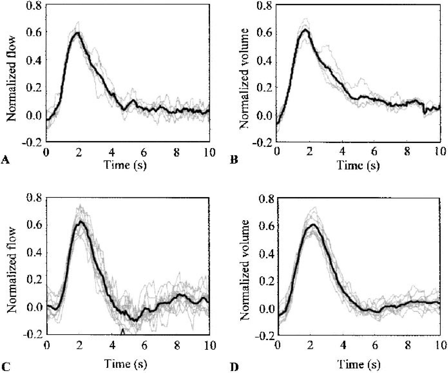
Hemodynamic impulse response estimates.
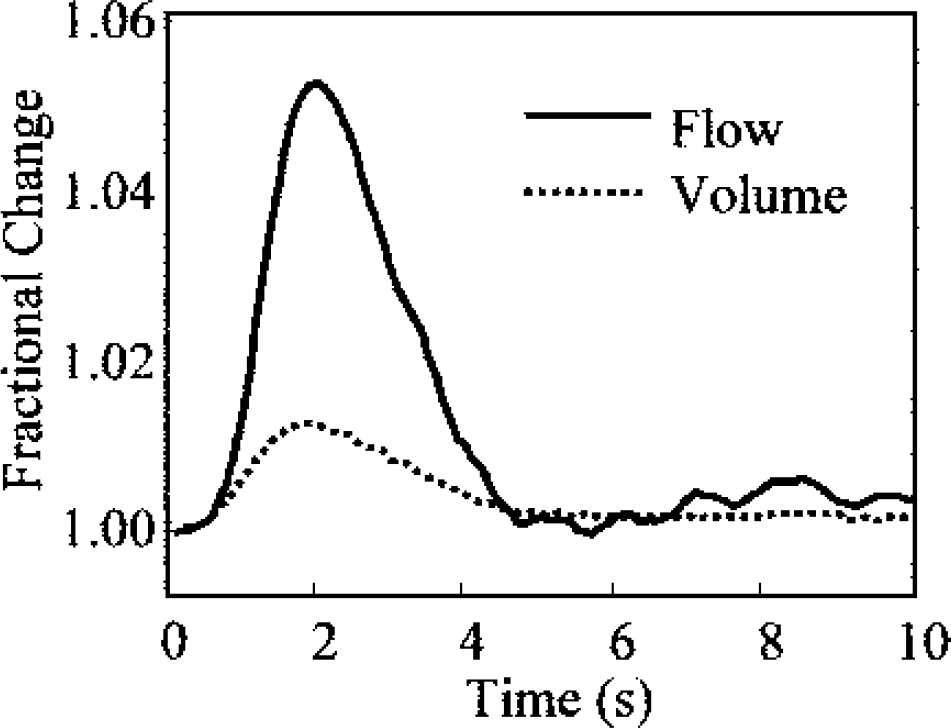
Hemodynamic impulse responses expressed as fractional changes after calibration. Figure shows blood volume and blood flow changes.
γ-Variate fits to rescaled hemodynamic impulse responses.
The scale of the results shown in Fig. 6 is a function of the normalization scheme: in essence, the peak impulse responses are roughly 60% of the normalized peak response to a 2-second, 1-Hz stimulus. To map the normalized impulse response functions to fractional changes in hemodynamic parameters, we used the peak magnitudes of the unnormalized hemodynamic responses to a 2-second, 1-Hz stimulus as the best estimates of the appropriate scaling factors. To obtain fractional changes from OIS data, we assumed a baseline hemoglobin concentration of 100 μmol/L (Mayhew et al., 2000). Figure 7 shows the impulse response fractional changes in volume and flow after rescaling. The rescaled impulse response functions show that the flow impulse response is approximately five times bigger than the volume impulse response (≈5% versus ≈1%, Fig. 7).
Applications I: modeling the hemodynamic impulse response
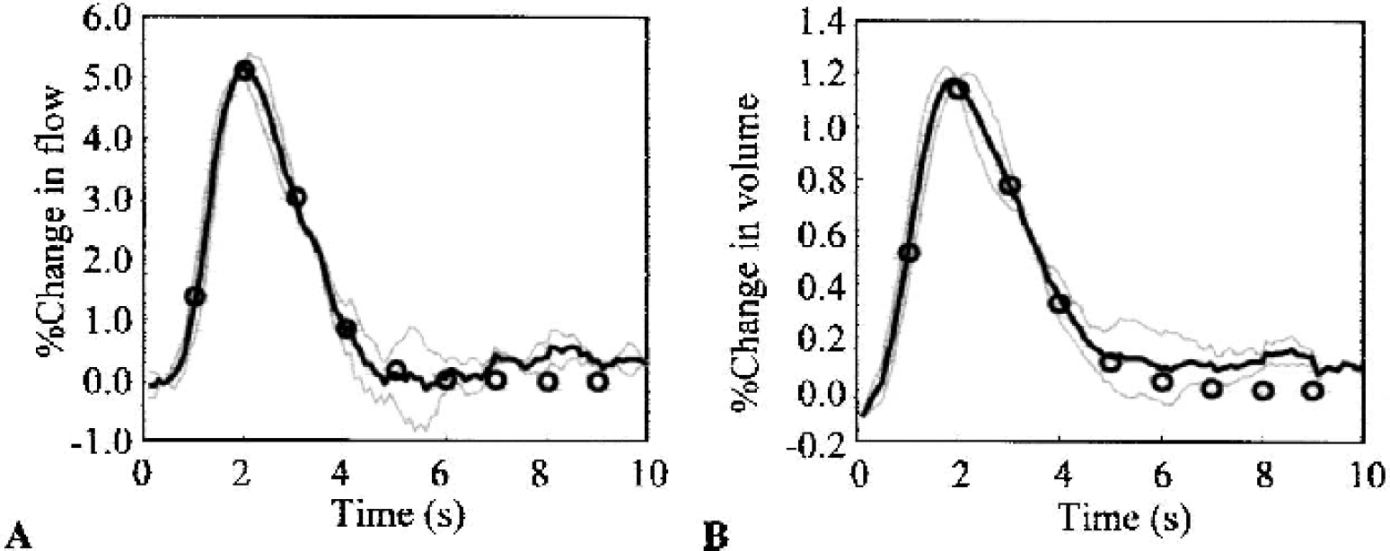
The hemodynamic response to stimulation is often modeled using a sum-normalized γ-variate, since each data time series can be reduced to the three parameters of mean, width, and amplitude (Cohen, 1997). To see if this approach is justified in the case of hemodynamic impulse response functions, a γ-variate model was fitted to the grand mean of all 16 impulse response estimates by using a nonlinear least squares algorithm (Levenberg-Marquardt algorithm, Matlab function “lsqnonlin”). Figures 8A and 8B show the grand mean (solid black line) and the γ-variate fit (solid circles) for flow and volume impulse responses, respectively. The means from the frequency and paired pulse data sets are also shown for comparison (gray lines). The γ-variate functions provide excellent fits to the data, with the parameters reflecting the slightly later time-to-peak and broader distribution of the volume impulse response.
An alternative approach to modeling the hemodynamic response to stimulation is to provide an explicit continuous time model. This approach has the advantage that the parameters defining the function can be more meaningfully interpreted. Recent attempts to model the response to stimulation from stimulus input to BOLD output (Friston et al., 2000; Zheng et al., 2001) have used a linear second-order step to relate “neural activity” to flow responses. Preliminary fitting of the impulse response estimates presented here indicates that the data are best fitted by a linear fourth-order continuous time function, the characteristics of which are currently being studied. This fourth-order system can be used to refine both modeling schemes.
Applications II: Grubb's power law
The power law relation between flow and volume changes (Grubb et al., 1974) shown in Eq. 4 is widely used in biophysical models of the BOLD response to stimulation (e.g., Davis et al., 1998; Hoge et al., 1999) for both extended and transient stimulus regimens.
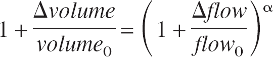
(Δ indicates change, subscript 0 denotes baseline, and α is a scaling constant). To examine whether a power law model is suitable during impulse response conditions, a value of α was estimated from least squares fitting of the logged time series. The flow changes estimated using Grubb's law followed the empirically derived flow changes very closely (r2 = 0.93) except in the longer return to baseline (Fig. 9). The value of α calculated from the current data was 0.23, which is comparable to reported values of 0.18 (Mandeville et al., 1999) and 0.31 (Jones et al., 2001). It is worth noting that a simple linear fit between volume and flow changes showed a slightly better fit than did the power law of Eq. 4 (raising r2 to 0.97; data not shown). Indeed, the power law of Eq. 4 can be well approximated as a linear relation because the fractional changes are reasonably small (<10%). Of particular interest is the close agreement between the temporal evolution of volume and flow changes. The remarkable similarity in width and time-to-peak of the flow and volume changes is in agreement with previously published data (Jones et al., 2001).
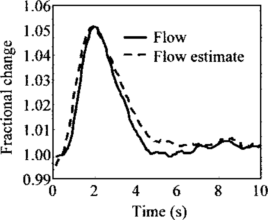
Estimation of blood flow changes from blood volume changes using a power law. Exponent was calculated as 0.23 by least squares fitting of logged response curves.
DISCUSSION
This study shows that the hemodynamic response to brief stimuli can be modeled as a linear convolution of a hemodynamic impulse response function with neural activity assessed by current source density. This conclusion confirms and extends the findings of Mathiesen et al. (1998) and Ngai et al. (1999), who report that peak hemodynamic activity is linearly related to the running sum of evoked field potential measurements. The present study may be extended by investigating the response to stimuli of longer duration. Whether the linear convolution model will explain the response to protracted stimuli will depend on possible nonlinearities introduced by hemodynamic effects. A hemodynamic refractory period well outside the neural refractory period has previously been reported (Cannestra et al., 1998; Huettel and McCarthy, 2000), suggesting that even if the mechanism underlying neural–hemodynamic coupling remains linear, the observed neural–hemodynamic coupling may not be linear. Ances et al. (2000) report a breakdown of a linear time-invariant model for stimuli of >8-second duration, suggesting that a linear neural–hemodynamic coupling may only exist during transient stimuli. These reports are consistent with our findings, which will be extended to studies of protracted stimuli in due course.
Metabolic costs of neural activation
The underlying mechanism by which hemodynamic responses to stimulation are triggered is still unclear; however, the prevailing opinion is that these responses serve the “metabolic needs of neural activation.” Quantifying the idea of “metabolic needs of neural activation” is itself an area of some dispute; however, recent studies are starting to shed light on the problem. A study by Sibson et al. (1998) shows a 1:1 relation between oxidative glucose metabolism and glutamate-neurotransmitter cycling. Since glutamate cycling is a measure of synaptic activity, and since energy consumption in cortex is dominated by excitatory glutamatergic signaling (87%) (Bonvento et al., 2002), this implies a 1:1 coupling between cortical oxidative glucose metabolism and synaptic activity. Since evoked field potentials measure primarily EPSP activity (Mitzdorf, 1985; Nakagawa and Matsumoto, 2000; Nicholson and Freeman, 1975), a coupling between EFP measurements (and hence CSD analysis) and oxidative glucose metabolism can also be inferred. Field potentials are a linear superposition of EPSPs but may appear nonlinear because of spread of the EPSP latencies. However, when averaged over a neural ensemble, it is to be expected that EFPs (and hence CSDs) will couple linearly to EPSP activity to a good approximation. A plausible conclusion is that current sinks and sources may be interpreted as linearly coupled to the oxidative glucose metabolism involved in excitatory, glutamatergic signaling. The present study attempts to extend this picture by showing that hemodynamic changes can be modeled as a linear function of current sink/source magnitudes. The tentative inference to be drawn from the above considerations is that hemodynamic changes (experimentally measured) are linearly related to oxidative glucose metabolism (as experimentally assessed through the quantification of current sinks and sources).
It has also been shown that fractional changes in neuronal oxidative metabolism have a 1:1 relation with fractional changes in neural spiking rate (Smith et al., 2002), from which it was inferred that hemodynamic changes are coupled to spiking rate. However, evidence that hemodynamic responses primarily reflect the metabolic needs of excitatory inputs is provided by the elegant study of Mathiesen et al. (1998). By modulating both inhibitory and excitatory inputs to Purkinje cells, they find hemodynamic responses to be independent of spiking rate but linearly related to summed field potential activity. These results suggest that inhibitory interactions may be metabolically “cheap.” Under conditions of tight coupling between afferent and efferent activity of a neuronal ensemble, hemodynamic responses will of course couple with both EPSP activity and spiking output.
Mechanisms underlying neural modulation
The frequency modulation and paired pulse paradigms were used to obtain a range of neural and hemodynamic response magnitudes. However, the CSD data have certain implications about the underlying neural modulation. First, both the frequency-dependent and paired pulse data show inhibition of the neural response within approximately 600 milliseconds of the first stimulus pulse. In addition, plotting the first two individual pulse responses from each frequency data set reveals an inhibition curve within the standard errors of that derived from the paired pulse experiments (data not shown). The similarity between the two data sets leads to the tentative hypothesis that the same neuromodulatory phenomena may be responsible for both effects.
Second, since there is a decrease in CSD magnitude, the data imply a decrease in afferent input to the cortex, rather than inhibitory intracortical interactions. This conclusion is consistent with several recent reports that identify a critical role for the thalamus in stimulus response modulation. Two of these reports find thalamic frequency-dependent response inhibition to diminish markedly during free whisking (Nicolelis and Fanselow, 2002) or during simulation of an awake state by injection of acetylcholine or stimulation of brain stem reticular formation (Castro-Alamancos, 2002). A further report suggests a major role for thalamocortical response conditioning combined with a role for intracortical response modulation (Chung et al., 2002). It therefore seems likely that the response modulation seen in cortical structures is more a reflection of thalamic processing than a property of the neocortex per se.
Recent work in this laboratory (Berwick et al., 2002) and elsewhere (Lahti et al., 1999; Peeters et al., 2001; Shtoyerman et al., 2000) has found much greater hemodynamic response magnitudes in unanesthetized animals as compared with anesthetized animals. In addition, neural modulation of the response to repetitive stimuli has been found to be much diminished in the awake (or simulated awake) state (Castro-Alamancos, 2002; Nicolelis and Fanselow, 2002). Thus, the much greater hemodynamic response observed in unanesthetized animals may simply reflect an increase in underlying cortical activity rather than an altered neural–hemodynamic coupling. Repetition of the present study in unanesthetized animals awaits completion of the necessary ongoing technical developments.
CONCLUSIONS
This study used general linear modeling to identify hemodynamic impulse response functions corresponding to a single “neural event.” The impulse response functions were estimated from two different data sets, and the estimates were found to be highly correlated. Peak flow and volume changes were approximately 5% and 1%, respectively, in response to a single neural event, which was in turn caused by a single electrical stimulus pulse of 0.3-millisecond duration at 1.2 mA. These data and analyses imply that neural–hemodynamic coupling during transient electrical stimuli can be modeled as a linear convolution of an impulse response function with a suitable train of “neural events.” Since the “neural events” used were current sinks, it is proposed that the hemodynamic impulse responses identified serve to support the metabolic costs involved in producing excitatory postsynaptic potentials.
Footnotes
Acknowledgments:
The authors thank the Center for Neural Communication Technology (University of Michigan), and the NIH grant that supports them, for supply and assistance with multichannel electrophysiology probes.