
Abstract
Recent studies have shown that the haemodynamic responses to brief (<2 secs) stimuli can be well characterised as a linear convolution of neural activity with a suitable haemodynamic impulse response. In this paper, we show that the linear convolution model cannot predict measurements of blood flow responses to stimuli of longer duration (>2 secs), regardless of the impulse response function chosen. Modifying the linear convolution scheme to a nonlinear convolution scheme was found to provide a good prediction of the observed data. Whereas several studies have found a nonlinear coupling between stimulus input and blood flow responses, the current modelling scheme uses neural activity as an input, and thus implies nonlinearity in the coupling between neural activity and blood flow responses. Neural activity was assessed by current source density analysis of depth-resolved evoked field potentials, while blood flow responses were measured using laser Doppler flowmetry. All measurements were made in rat whisker barrel cortex after electrical stimulation of the whisker pad for 1 to 16 secs at 5 Hz and 1.2 mA (individual pulse width 0.3 ms).
Introduction
The mechanisms by which haemodynamic responses are coupled to neural activation remain incompletely characterised. Since many neuroimaging techniques (most notably fMRI) use haemodynamic measurements as a surrogate for measurements of neural activity, understanding of this coupling is critical for accurate data interpretation. Recently, we reported that a simple linear convolution of neural activity with an identified haemodynamic impulse response provided a good characterisation of the observed haemodynamic responses over the range of stimuli tested (1 to 5 Hz, 2-sec duration). If this model were found to be generally applicable, it would greatly simplify data analysis, since neural activity could be linearly related to haemodynamic responses. However, there are many reports of nonlinearity in haemodynamic responses in the literature (e.g. Ances et al, 2000; Huettel and McCarthy, 2000; Miller et al, 2001; Pfeuffer et al, 2003; Vazquez and Noll, 1998), and so it is unlikely that a simple linear convolution model (LCM) is general.
One method of inducing nonlinearities in the haemodynamic response is to use stimuli of different durations. Although some studies find the haemodynamic response to be linear (Boynton et al, 1996), most BOLD fMRI studies in humans have found the haemodynamic response to be nonlinear with brief stimuli (<2- to 4-sec) and linear for longer stimuli (e.g. Vazquez and Noll, 1998; Pfeuffer et al, 2003; Soltysik et al, 2004). Since these studies have been conducted without a complementary neural measure, it is not known whether these nonlinearities are because of the coupling between stimulus input and neural activity or that between neural activity and haemodynamic changes. In contrast, animal studies can measure both neural activity and flow responses. For example, Ances et al (2000) found that, taking into account neural nonlinearities, responses to brief stimuli (<4 secs) were linear, while responses to longer stimuli were better explained by a nonlinear model. Similarly, our previous work (Martindale et al, 2003) found the response to brief stimuli to be well modelled by a linear convolution of measured neural activity with a haemodynamic impulse response. An attempt to explain the apparent contradiction between human and animal studies can be found in the discussion.
The coupling between neural activity and haemodynamics is thought to be due to a primary active coupling between neural activity and blood flow changes, with a further passive mechanism linking blood flow and blood volume changes (e.g., Buxton et al, 1998; Friston et al, 2000; Mandeville et al, 1999). This paper reports attempts to model the first of these relationships (that is, between neural activity and local blood flow changes); however, in the experiments described, both laser Doppler flowmetry (LDF) data (yielding blood flow changes) and optical imaging spectroscopy data (yielding blood volume changes) were acquired concurrently. Identification of a nonlinear system describing the second relationship (the coupling between flow and volume changes) based on the insights of Mandeville et al (1999) and Buxton et al (1998) is described elsewhere (Kong et al, 2004).
The measurement techniques employed here (current source density (CSD) analysis of evoked field potentials and LDF) are particularly well suited for a study of the coupling between neural activity and blood flow responses. Current source density analysis resolves the spatial ambiguities inherent in evoked field potential recordings into a laminar distribution of current sinks and sources. The primary current sink has previously been found to colocalise extremely well with layer IV as visualised by cytochrome oxidase histology (Jones et al, 2004). A recent autoradiography study (Gerrits et al, 2000) has shown that maximal CBF (both at rest and during stimulation) is also observed in layer IV. Thus, CSD data and LDF data (which is a spatial average over depths) have their major signal sources colocalised in layer IV.
The purpose of this study was to test whether the previously identified LCM (or indeed any LCM) could adequately predict the blood flow responses to stimuli of long (>4 secs) duration. Having found a LCM to be inadequate, we implemented both a recently published second-order linear control system (Rosengarten et al, 2003) and a more heuristic nonlinear model. The second-order linear system was found to provide a poor fit to the post-stimulus data. In contrast, the nonlinear convolution model was found to provide a good fit to the data over the whole response.
Materials and methods
Since the current work is in large part an extension to a previous study (Martindale et al, 2003), much of the methods used are the same and the reader is directed to the previous work for more complete methodological details.
Animal Preparation
Hooded Lister rats weighing between 250 and 400 g were kept in a 12-h dark/light cycle environment at a temperature of 22°C with food and water ad libitum. Before surgery, animals were anaesthetised with urethane (1.25 g/kg intraperitoneally) with additional doses (0.1 mL) administered if necessary. Atropine was also administered (0.24 mg/kg subcutaneously) to reduce mucous secretions during surgery. Rectal temperature was maintained at 37°C throughout surgical and experimental procedures using a homeothermic blanket (Harvard). Animals were tracheotomised to allow artificial ventilation and measurement of end-tidal CO2. The femoral vein and artery were cannulated to allow drug infusion and measurement of mean arterial blood pressure, respectively. Animals were placed in a stereotaxic frame (Kopf Instruments). Physiological parameters were continuously monitored and maintained within normal ranges (pO2=83.3±5.9, pCO2=35.6±8.3, MaBP=103.5±3.1, mean±standard deviation across all animals). All procedures were performed in accord with Home Office regulations.
Data Acquisition
Animals were used for either LDF measurements (nine animals) or electrophysiology measurements (six animals), yielding a total of 15 animals in the study. Before blood flow measurements (n=9), the skull overlying the somatosensory cortex was thinned to translucency with a dental drill under constant cooling with saline. A plastic ‘well’ was attached to the thinned skull and filled with saline (37°C) to reduce specularities from the skull surface. The LDF probe was positioned normal to the cortical surface, with care being taken to avoid any visible large vessels. For electrophysiological measurements (n=6), the skull overlying the somatosensory cortex was removed completely, and the dura overlying the chosen barrel area was removed. The multielectrode probe was then inserted normal to the cortical surface under micromanipulator control.
Stimulus Presentation and Paradigms
All stimulus presentation was controlled through a 1401plus (CED Ltd, UK) running custom-written code with stimulus onset time locked to either the CCD camera or the electrophysiology recording unit. Electrical stimulation of the whole whisker pad was delivered via tungsten electrodes inserted in an anterior direction on each side of the whisker pad. All electrical stimuli were presented at 1.2 mA with a 0.3-ms individual pulse width at a rate of 5 Hz. Stimuli were presented for durations of 1, 2, 4, 8, or 16 secs and were randomly interleaved with an interstimulus interval (defined as the time from the end of one stimulus to the start of the next) of 45 secs. This very long ISI was used to ensure that there were no interaction effects between adjacent stimuli. Each animal was presented with 30 trials per condition and the stimulus design was the same for both optical and electrophysiological measurements.
Localisation of Activated Region in the Barrel Cortex
Somatosensory cortex was monochromatically illuminated at 590 nm (narrow bandwidth interference filter, ±5 nm) and images were recorded using a 12-bit CCD camera (SMD 1M60). The whisker barrel cortex was located by electrically stimulating the entire whisker pad (5 Hz, 1 sec, 1.2 mA). In all, 30 trials were collected at 15 Hz, each of 12 secs duration, stimulus onset at 8 secs, 15 secs inter-stimulus interval. Images were analysed using a variation of a signal-source separation algorithm (Molgedey and Schuster, 1994) exploiting a weak temporal model, as previously described (Zheng et al, 2001). The resultant barrel activation maps were registered with images of cortical surface to guide insertion of the electrophysiology probe. Localisation of the barrel cortex using this method has been shown to exhibit excellent concordance with cytochrome oxidase histology (Jones et al, 2001, 2002; Zheng et al, 2001).
Laser Doppler flowmetry and Electrophysiology
Laser Doppler flowmetry provides a measure of blood flow by quantifying the Doppler shift imparted to incident photons by moving blood cells. After localisation of barrel cortex, an LDF probe (PeriFlux 5010, Perimed, Stockholm, 780 nm illumination, 0.25 mm separation) was placed over the area of interest. Visual inspection of cortical surface through the translucent thinned skull preparation allowed large vessels to be avoided during placement of the LDF probe. The signal from the LDF probe was analysed by an LDF spectrometer, which includes a proprietary linearisation algorithm (Nilsson, 1984) to reduce errors caused by changes in blood volume. The LDF signal was then digitised continuously using a 1401plus (CED Ltd, UK). The time constant of the LDF recordings was 0.2 secs, and the bandwidth was 12 kHz.
Laminar recordings of evoked field potentials were made using a multielectrode probe with 16 recording sites on a single shaft (100 μm intersite spacing, area of each site 177 μm2, impedance 1.5 to 2.7 MΩ, probe width: 33 μm tip, 123 μm at uppermost electrode; CNCT, University of Michigan). The probe was inserted under micromanipulator control until the uppermost electrode just penetrated the cortical surface. Recordings were averaged over 30 trials for each stimulus condition, with stimulus onset ‘jittered’ within a 20 ms window to reduce the effects of 50 Hz mains noise. The measured evoked field potentials were digitised at 6kHz with 16-bit resolution using a ‘Medusa Bioamp’ (TDT, Florida) driven by a custom-written Matlab (The Mathworks Inc., USA) interface. The data were subjected to CSD as described previously (Martindale et al, 2003, see also Mitzdorf (1985) and Rappelsberger et al (1981) for a more general discussion). Assuming homogeneity and anisotropy of the rat barrel cortex, a one-dimensional CSD equation can be applied to depth-resolved field potentials to estimate the underlying current sinks and sources. The data were subsequently interpolated and filtered to give an apparent spatial resolution of 50 μm.
Current Source Density Data Preprocessing
Preliminary analysis of the CSD data was identical to that described previously (Martindale et al, 2003). Since the spatial pattern of activation did not vary across stimuli, the first principal component (accounting for >80% of the variance in every data set) was used to collapse the data across the spatial dimension, yielding one time series per stimulation condition. Since the responses to individual stimulus pulses were resolvable as scaled copies of one another, the absolute value of the current sink depth after each stimulus pulse was used to represent the data. The first pulse response to each stimulus was then normalised to unity (see Figure 1).
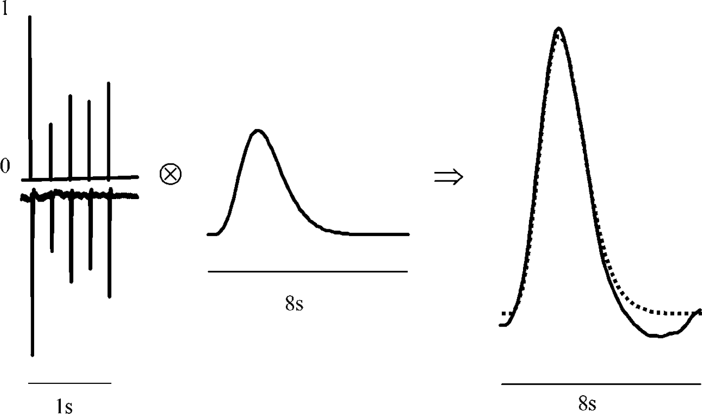
Schematic of LCM. Neural activity is represented as delta functions normalised to a single 0.3ms 1.2 mA pulse response. Neural activity is then convolved with an impulse response to yield a model (dashed line) of the data (solid line).
Linear Convolution Modelling
The LCM is shown diagrammatically in Figure 1 and represented mathematically as
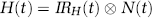
where H(t) is the haemodynamic response, IR H (t) is the haemodynamic impulse response and N(t) is the neural activity. The neural activity is convolved with a haemodynamic impulse response, and the result of this process models the data. The impulse response functions can be obtained either by measurement or by deconvolving more complex stimuli by putting the known neural and haemodynamic responses into a general linear model. The advantage of the latter method is that a substantial increase in signal to noise can be obtained. An impulse response for flow changes was previously obtained (Martindale et al, 2003) and found to be excellently modelled as a gamma-variate function:
where δ is the mean, τ the width, and C the scaling constant (previously identified flow impulse response: δ=2.37 secs, τ=0.76 secs, and C=10.6).
In applying the LCM to the current data, there were two questions which we wished to ask. Firstly, could the previously obtained LCM (i.e. convolution of the neural activity with the previously obtained impulse response) be used to fit the data? Secondly, is there any LCM (i.e. convolution of the neural activity with some new impulse response) which would fit the data? In practice, both questions can be answered using the same method. For each stimulus duration, a design matrix was constructed in which the neural activity was used to weight the inputs, and the shape of the estimated finite impulse response was unconstrained: thus a finite impulse response of n time-points duration consisted of n estimated parameters. If the resulting impulse response could be convolved to model the data, then a LCM was applicable. Furthermore if the impulse responses were identical to the previously identified impulse responses, then the LCM was the same as the previously obtained model.
Second-Order Linear System Modelling
During the acquisition of data for the current study, a control theory approach to modelling the blood flow responses to long stimulation was proposed by Rosengarten et al (2003). We implemented their second-order linear system and used nonlinear least-squares optimisation to obtain parameters for the current data set, using a simple step input as the stimulus. Our parameters were all within one standard deviation of those reported in Rosengarten et al (2003) for 0.3-ms pulses, with the exception of natural frequency, indicating that we were indeed modelling very similar responses (our parameters: τD=1.32 secs, K=15.29%, ξ=0.58, τ v =3.42 secs, ω=1.56 secs−1).
Nonlinear Convolution Modelling
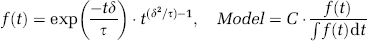
The LCM of Equation (1) was modified to include two independent but concurrent mechanisms: one impulse response convolved linearly with the neural activity; another impulse response convolved with neural activity multiplied by some weighting function W(t):

The modified convolution model of Equation (3) is shown schematically in Figure 2. Inspection of the data suggests a weighting function which is initially high but rapidly decays to zero. Somewhat heuristically, the weighting function was assumed to have the form:
Schematic of the modified, nonlinear convolution model.
An exponential decay was chosen as the weighting function because of its mathematical simplicity and few parameters.
Unlike the LCM, the parameters of the nonlinear convolution model could no longer be estimated using general linear modelling. Instead, a Levenberg–Marquardt algorithm for nonlinear least-squares minimisation (Matlab optimisation function ‘lsqnonlin’) was used to optimise the free parameters of the model, with the impulse responses being modelled as gamma-variate functions (equation (2)). This gave a total of seven free parameters to fit (three for each impulse response and a time constant for the exponential weighting). The entire data set was used in the parameterisation of the model, and the error function was constructed to fit the responses from stimulus onset to response cessation (so as to model the entire blood flow response but avoid fitting baseline noise). Response cessation was empirically judged to occur at approximately 7 secs after stimulus cessation in the maximum duration (16 secs) case; thus, a period equal to stimulus duration plus 7 secs was used to generate the error functions.
Results
Neural Responses
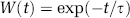
For each stimulation, there was a neural response to each individual stimulus pulse. The neural responses to stimulus pulses showed rapid suppression to ∼30% of the initial pulse response amplitude and a subsequent rise to a stable level of ∼50% of the initial pulse response amplitude (Figure 3a). Overlaying the first second of each stimulus response showed that an identical pattern of activity was seen regardless of the stimulus duration. Furthermore, this pattern of activity was found to be within one standard deviation of previous data (Martindale et al, 2003; 2 secs, 5 Hz stimulus, data not shown). These results show there to be a consistent, nonlinear relationship between stimulus input and neural activity.
Data. (
Blood Flow Responses
In contrast to the neural data, responses to individual stimulus pulses were not resolvable in the blood flow data; rather, a single blood flow response was observed for each stimulus duration (Figure 3b). The responses to all stimuli peaked between 2 and 4 secs and the amplitude of the initial peak increased monotonically with stimulus duration up to 4 secs, before asymptoting at ∼25% for the 4-, 8- and 16-sec stimuli. However, after their initial peaks, the responses to 8- and 16-sec stimuli decreased to ∼50% of their peak deflections. This ‘peak and plateau’ pattern of response is consistent with our previous data (Jones et al, 2002) and that of others (Ances et al, 2000; Rosengarten et al, 2003; Ureshi et al, 2004).
Linear Convolution Model
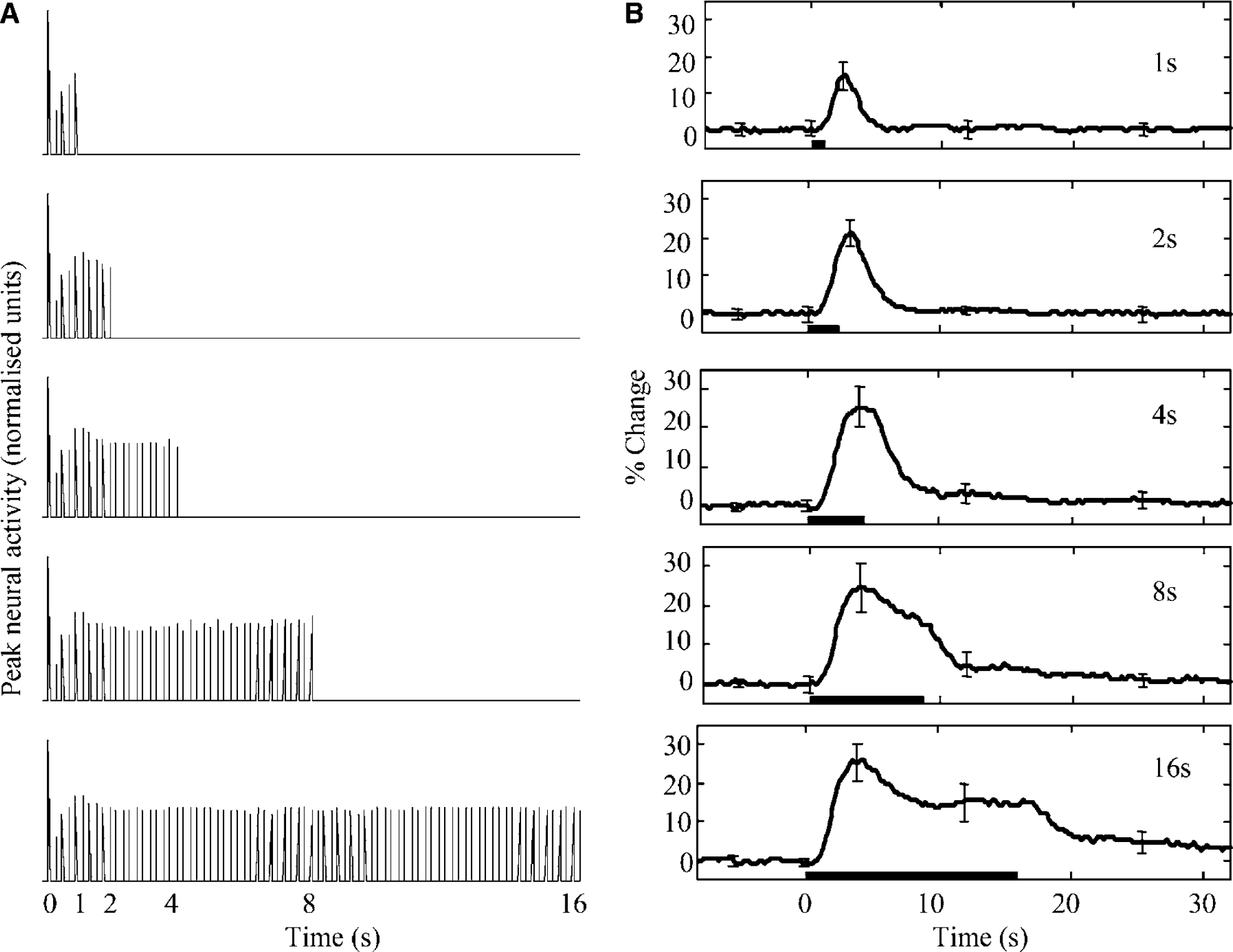
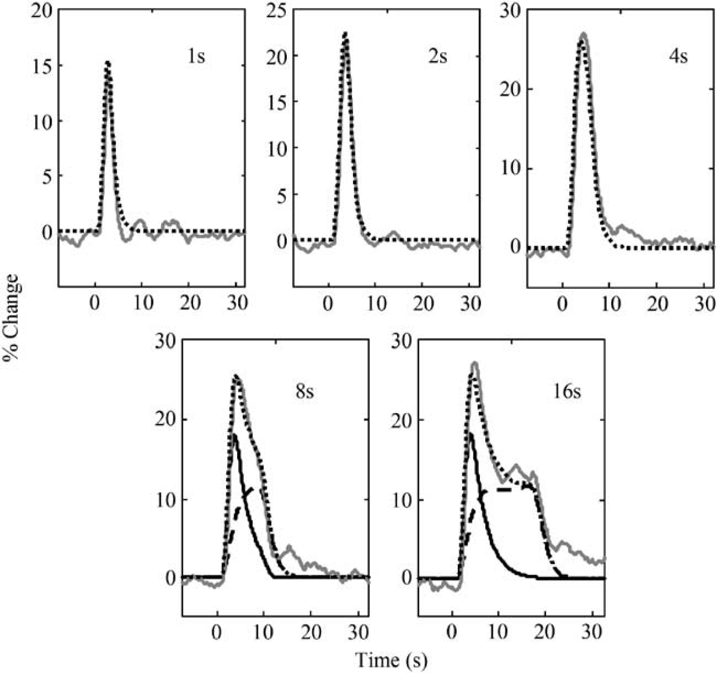
Figure 4 shows the LCM fits to the data for each stimulus duration, using unconstrained impulse responses. It is clear that while the 1-, 2- and 4-sec stimulus responses are well characterised by the LCM, the model gives a much poorer fit to the responses to 8- and 16-sec stimuli. It is important to note that unlike many deconvolution schemes, the design matrix used to deconvolve the impulse response explicitly contained information about the neural activity. Thus, the poorness of fit for the extended stimuli could not be ascribed to a nonlinearity in the relationship between stimulus input and neural activity; rather, the nonlinearity seen in the responses to 8- and 16-sec stimuli must have its origin in the coupling between neural activity and the blood flow responses.
Comparison of unconstrained linear model (dotted black lines) with observed responses (solid grey lines) for stimuli of different durations.
The mean impulse response derived from the 1 to 4 secs stimuli was compared with the flow impulse response previously identified in Martindale et al (2003) (equivalent to equation (2) with δ=2.37 secs, τ=0.76 secs, and C=10.6). There was a high degree of agreement between the two impulse response estimates (r2=0.96, data not shown), indicating that the responses to the 1 to 4 secs stimuli could be well modelled by the previously identified LCM. Above 4 secs duration, the LCM was inadequate.
Sccond-Order Linear System Modelling
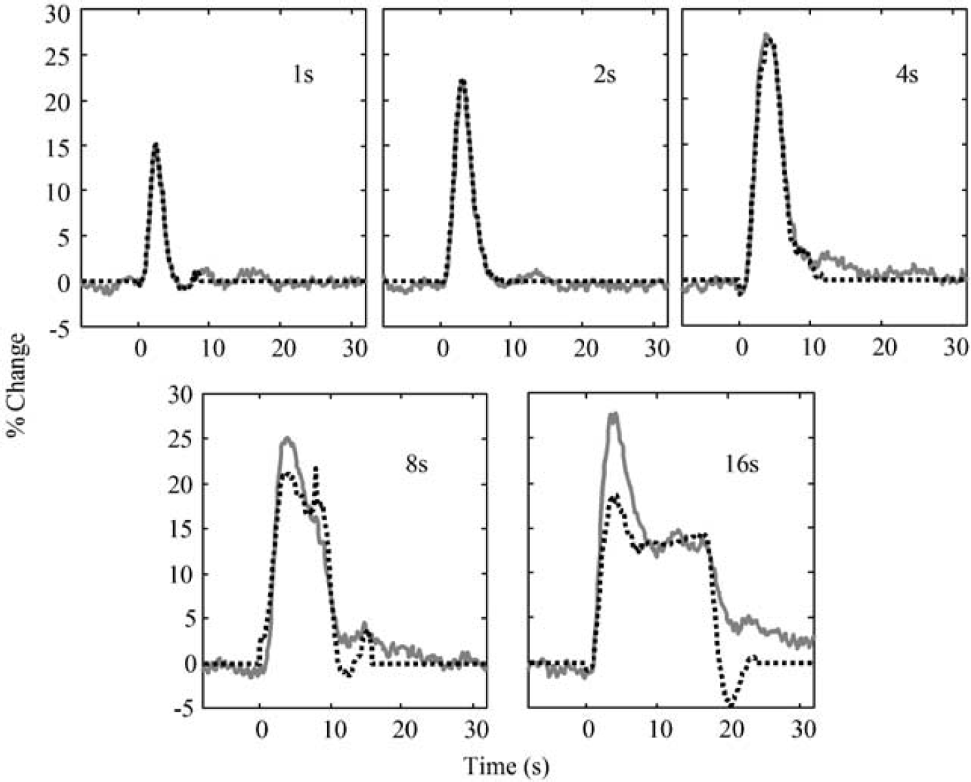
This model provided an excellent fit to the peak and plateau of the responses (Figure 5 shows the 16-sec stimulus data and model), but a very poor fit to the data after stimulus cessation. In fact, the pronounced undershoot in the modelled data after stimulus cessation is a necessary consequence of the second-order linear system: any sudden change (either stimulus onset or cessation) necessarily causes a transient in the response. The more heuristic nonlinear convolution model we propose (equation (3)) does not have this problem and provided an adequate fit to the data throughout the stimulation period.
Comparison of measured data (solid grey line) with second-order linear system (dashed black line) for a 16-sec stimulation. The model fits extremely well during stimulation, but extremely poorly after stimulus cessation.
Nonlinear Convolution Modelling
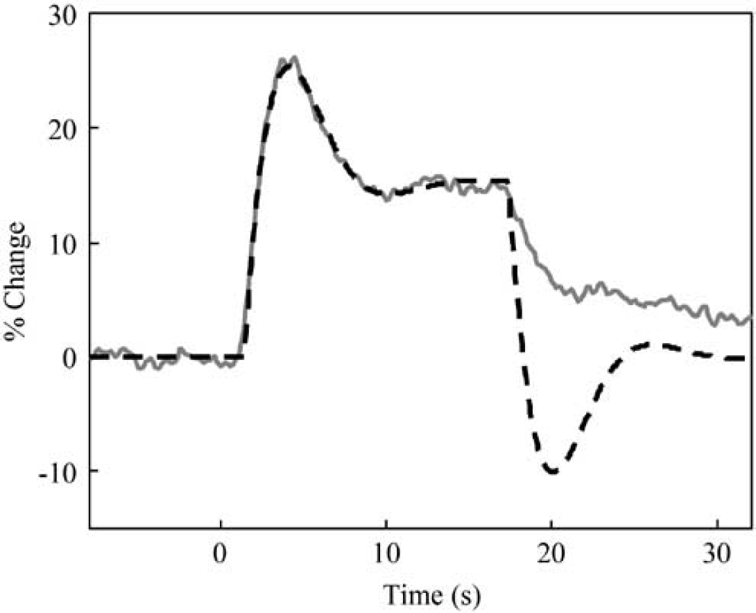
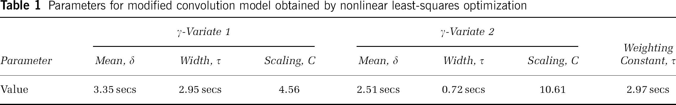
Optimisation of the nonlinear convolution model yielded the parameter values shown in Table 1. The fits of the nonlinear convolution model (dotted lines) to the LDF data (solid grey lines) are shown in Figure 6, along with the contributions of the two impulse response convolutions. The goodness of fit is high across all stimulus durations, as shown by the r2 values (0.87 to 0.95); however, there is a slight difference between the modelled and real data in the post-stimulus return to baseline for the 16-sec stimulus condition. This may reflect some contamination of the ‘active’ neural-flow coupling with some ‘passive’ venous effects.
Comparison of modified convolution model (dotted black lines) with LDF measured blood flow responses (solid grey lines). Also shown on the responses to 8- and 16-sec stimuli are the contributions from the ‘brief’ impulse response (solid black lines) and the ‘general’ impulse response (dashed black lines).
Parameters for modified convolution model obtained by nonlinear least-squares optimization
To test the generality of the model, data from a previous study which were well explained by the LCM (see Martindale et al, 2003) were re-analysed using the modified model. An acceptable fit was found under all stimulus conditions, with r2>0.91 in all cases (data not shown). The values of r2 followed no discernible pattern, indicating that deviations from the model were not systematic. The modified convolution model is able to model data from a wide range of different stimulation paradigms.
Figure 7 shows the impulse responses identified in the nonlinear convolution model, along with the exponential weighting term. Also shown is the impulse response function previously identified for the LCM for 2-sec 1 to 5 Hz stimuli. The term ‘general’ impulse response is used to denote IR 1 of equation (3) (convolved with neural activity), the ‘brief’ impulse response is taken to refer to IR 2 (convolved with exponentially weighted neural activity) and the ‘linear’ impulse response refers to the impulse response previously identified in Martindale et al (2003). Interestingly, the ‘linear’ and ‘brief’ impulse responses are very similar both in amplitude and in time course, while the ‘general’ impulse response is broader, with a longer latency and smaller amplitude. In Figure 6, it is apparent that the ‘general’ impulse response has little contribution to the early (<3 secs) ‘peak’ response, but dominates the later ‘plateau’ response. The similarity of the ‘brief’ and ‘linear’ impulse responses shows why a LCM can seem appropriate for brief (<4 secs) stimuli. Furthermore, these results suggest that the ‘peak’ and ‘plateau’ responses could be because of two independent and (in principle) separable mechanisms.
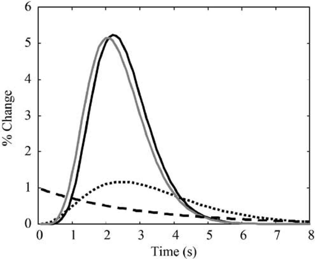
Previously identified impulse response (solid grey line) is almost identical to ‘brief’ impulse response in the modified convolution model (solid black line). The ‘general’ impulse response (dotted black line) is broader, of lower amplitude and longer latency. Also shown is the weighting function (dashed black line).
Discussion
Advantages of the Nonlinear Convolution Model
The nonlinear convolution model provides substantially better fits to the data (Figure 6) than either our previous LCM (Figure 4) or the second-order linear system of Rosengarten et al (2003) (Figure 5). Since most of the neural responses have the same amplitude (approximately half the initial stimulus pulse response amplitude), linear convolution cannot predict the ‘peak-and-plateau’ response pattern observed. The second-order linear system can predict the ‘peak-and-plateau’ response, but at the expense of a very poor prediction of the return to baseline phase of the response. The nonlinear convolution model we propose here effectively separates the ‘peak’ and ‘plateau’ components of the response and thus can model the data extremely well.
Previous authors have also found nonlinear components to be essential to model blood-flow responses from neural activity for longer (>4 secs) stimuli (Ances et al, 2000). The advantage of our current convolution approach is that each and every neural response is used in the modelling in an intuitive and physiologically interpretable manner.
Weighting Function and Nonlinear Convolution Model
As noted in the methods section, the choice of weighting function was somewhat arbitrary and so the interpretation that the model is somehow ‘true’ or ‘correct’ must be treated with care. Two variations on the model of equation (3) were also evaluated. In the first, the weighting function was a simple on–off switch function. The exact time of the switch was set manually, since the minimisation algorithm cannot operate on discrete functions. In the second variation, the impulse responses IR 1 and IR 2 were constrained to be identical,

with a weighting function of the form,
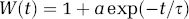
The weighting function is simply an exponential decline to a steady-state level, and the relative scaling between the exponential decay and the stable baseline is now parameterised by a rather than the relative amplitudes of the impulse responses. While both variations gave reasonable fits to the data (r2>0.8 for all data sets), neither variation was as good (in terms of r2 scores) as the model expressed in equation (3).
A further problem with the nonlinear convolution model of equation (3) is that the weighting function must be ‘reset’ for each stimulus train: that is, for two ‘well separated’ (e.g. ISI >∼2 secs) trains of stimulus pulses, the t of equation (3) must be reset to zero. This makes the translation of the model into control theory terminology somewhat difficult. We conjecture that a weighting function which takes into account the recent history of the neural input might be able to approximate an exponential decline over a short period of stimulation, but would ‘recover’ after a period of no stimulation. A weighting function of this form might even be able to account for ‘refractory’ behaviour. The plausibility and form of this kind of weighting function are ongoing research topics.
Origin of the Neural–Haemodynamic Nonlinearity
One noticeable feature of response nonlinearities is that they appear to be region specific. For example, both Soltysik et al (2004) and Pfeuffer et al (2003) find the nonlinearity in the BOLD response to vary as a function of spatial region and the latter study also finds the degree of BOLD nonlinearity to vary as a function of magnetic field strength. Pfeuffer et al (2003) argue that the early onset responses correspond to grey matter, while longer latency responses are of vascular origin, implicating the specific tissue type (capillaries versus larger vessels) as the source of response nonlinearity. Unpublished observations (Berwick, personal communication, 2004) show that the ratio of peak to plateau in the blood volume responses to 16 secs electrical stimuli is greater in arteries than in either parenchyma or veins, lending support to the idea that tissue type might be implicated in response nonlinearities.
However, this cannot be the whole story, since studies performed within a single region of tissue can observe different nonlinearities depending on the stimulus used. Laser Doppler flowmetry measurements are necessarily made from a well-mixed compartment, and the composition of this compartment does not change substantially through an experiment. Examination of the LDF responses to rat hindpaw stimulation shown in Figure 1 of Ureshi et al (2004) or Figure 7 of Matsuura and Kanno (2001) shows that for 15-sec stimuli at 1 Hz (0.1 ms pulse width) only a ‘plateau’ response is seen, while at 5 Hz a ‘peak and plateau’ response is seen and at 10 Hz only a ‘peak’ is seen. However, in those studies, it is unclear how much of this nonlinearity can be accounted for by the relationship between stimulus and neural activity. An interesting finding in the work of Rosengarten et al (2003) is that the response to electrical stimulation of the forepaw in rat shows the characteristic peak-and-plateau response for an individual pulse width of 0.3 ms, while for an individual pulse width of 5 ms only a plateau response is seen. Concurrent local field potential recordings showed no difference, indicating that the difference in response was not because of neural activity. Thus, the neural–haemodynamic nonlinearities can change even within the same region of tissue and with identical neural activity.
The control system approach taken in the work of Rosengarten et al (2003) finds two mechanisms in the ‘peak and plateau’ response and attributes these to a feedforward (peak response) and a feedback (plateau response) mechanism. These findings are similar to our own (‘brief’ and ‘general’ impulse responses), although couched in different mathematical terminology. The idea of two (or more) independent and complementary systems mediating the neural–haemodynamic coupling is one which appears to allow for modelling of the data, but which is as yet lacking a basis in neurophysiology.
Currently, neither the mechanism(s) mediating the cerebral blood flow response to neural activation, nor the site(s) at which these mechanisms act, are known for certain. Both nitric oxide (NO) and adenosine have been implicated in neural-flow coupling (Dirnagl et al, 1994), and a more recent study has implicated both NO and epoxygenase as potential mediators of the neural-flow coupling (Peng et al, 2004). Neither of these studies found a simple additive relationship between the mediators investigated and blood flow response, indicating that there is a rather complex interaction which may involve further mediators. Recent research into the origin of the mechanism(s) signalling blood flow changes has strongly implicated astrocytes as a potential site of a mediating signal (Zonta et al, 2003a, 2003b). The fact that epoxygenase (CYP2C11) is expressed in astrocytes in rat cortex (Peng et al, 2004) provides further evidence of the role of astrocytic processes in the neural-flow coupling; however, a role for other site(s) (e.g. vascular smooth muscle) in the neural-flow coupling cannot be ruled out. These results suggest the speculative hypothesis that the ‘peak’ and ‘plateau’ responses reported and modelled in the current paper might be because of differences in time courses of different mediators of the neural-flow coupling. Alternatively, the ‘peak’ and ‘plateau’ responses might be because of differences in the physical properties of the sites at which mechanisms act (e.g. vascular smooth muscle versus astrocytic processes). Further research in this area is necessary to decide which (if any) of these hypotheses is correct.
Discrepancy Between Human and Animal Studies
As noted in the introduction, most human fMRI BOLD studies find the response to brief stimuli to diverge from linearity, whereas there is good evidence in animal studies for claiming that response nonlinearities only become apparent at longer stimulus durations. It seems that this apparent divergence can be ascribed simply to the different analysis approaches taken.
In animal studies, a concurrent neural measure is often taken, and the high temporal resolution of the measurement techniques (electrophysiology and usually LDF) allow the acquisition of responses to brief stimuli. As shown by us and others (Ances et al, 2000; Martindale et al, 2003; Ngai et al, 1999) these responses can be well characterised by a linear model. When extending this finding to stimuli of longer duration, the linear model fails to predict the data and so the responses to long stimuli are termed ‘nonlinear’. Due to the lower temporal resolution and signal-to-noise of BOLD studies, responses to long duration stimuli are taken as the ‘gold standard’ and used to generate the impulse responses (usually with neural activity assumed to be represented as a simple step-function). This linear model does not work for brief stimuli, and so those responses are termed ‘nonlinear’ in the fMRI literature. The present work shows that while nonlinearities in the neural responses must be taken into account, it is the responses to brief stimuli which are best characterised as nonlinear. As a caveat, it should be noted that LDF primarily measures capillary blood flow changes, while BOLD fMRI is more sensitive to venous effects. However, although this may introduce some intrinsic differences between the measured signals, the major signal characteristics are comparable.
The use of anaesthesia is known to affect the coupling between neural activity and haemodynamic changes (e.g. Smith et al, 2002) and may introduce a confounding effect between animal and human studies. However, inspection of a recent paper (Pfeuffer et al, 2003) shows the ‘peak-and-plateau’ response pattern described in the current paper to be present in awake humans, indicating that this response type is neither a function of anaesthetic nor of species. In the current study, every effort was made to keep anaesthetic depth constant across animals, as is evidenced by the extremely consistent data obtained. An awake animal preparation is currently under development (Berwick et al, 2002; Martin et al, 2002), which will allow further investigation of the effects of anaesthesia on neural–haemodynamic coupling.
Conclusion
The current study measured neural activity and blood flow responses to stimuli varying in duration from 1 to 16 secs at 1.2 mA and 5 Hz. Neural responses quickly (∼1 sec) reached a steady state at ∼50% of the initial response magnitude, while haemodynamic responses showed a distinctive ‘peak-and-plateau’ response. The LCM was unable to predict the responses to stimuli of duration greater than 4 secs; however, a nonlinear convolution model was able to predict the responses to all stimuli. In addition, the nonlinear convolution model was also valid for previous data sets. Since the nonlinearity in the coupling between stimulus input and neural activity is implicit in the modelling process, the nonlinearity in the modified convolution model must be because of a nonlinear neural–haemodynamic coupling. The works of Ureshi et al (2004), Rosengarten et al (2003) and Matsuura and Kanno (2001) indicate that simple manipulations of applied stimuli can induce changes in the neural–haemodynamic nonlinearities, and future work is planned to use these manipulations as an investigative tool.
Footnotes
Acknowledgements
This work was supported by EPSRC grant GR/R46274/01, MRC project grant G0100538, NIH grant 1R01NS044567–01, and an MRC research studentship. We gratefully acknowledge the technical staff of the laboratory (Marion Simkins, Natalie Walton, Malcolm Benn) for their assistance. We also gratefully acknowledge the Centre for Neural Communication Technology (University of Michigan), and the NIH grant which supports them, for supply and assistance with multi-channel electrophysiology probes. We thank both referees for their comments.