Sage Journals: Discover world-class research

Abstract

Functional hemodynamic responses are the composite results of underlying variations in cerebral oxygen consumption and the dilation of arterial vessels after neuronal activity. The development of biophysically based models of the cerebral vasculature allows the separation of the neuro-metabolic and neuro-vascular influences on measurable hemodynamic signals such as functional magnetic resonance imaging or optical imaging. We describe a multicompartment model of the vascular and oxygen transport dynamics associated with stimulus-driven neuronal activation. Our model offers several unique features compared with previous formulations such as the ability to estimate baseline blood flow, volume, and oxygen consumption from functional data. In addition, we introduce a capillary compliance model, arterial and venous oxygen permeability, and model the dynamics of extravascular tissue oxygenation. We apply this model to multimodal optical spectroscopic and laser speckle imaging of the rat somato-sensory cortex during nine conditions of whisker stimulation. By fitting the model using a psuedo-Bayesian framework to incorporate multimodal observations, we estimate baseline blood flow to be 94 (±15) mL/100 g min and baseline oxygen consumption to be 6.7 (±1.3) mL O₂/100 gmin. We calculate parametric, linear increases in arterial dilation (R² = 0.96) and CMRo₂ (R² = 0.87) responses over the nine conditions. Other parameters estimated by the model include vascular transit time and volume reserve, oxygen content, saturation, diffusivity rate constants, and partial pressure of oxygen in the vascular compartments and in the extravascular tissue. Finally, we compare this model to earlier work and find that the multicompartment model more accurately describes the observed oxygenation changes when compared with a single compartment version.

Keywords

CBF and oxidative metabolism human and experimental studies hemodynamics optical imaging and spectroscopy NIRS (near-infrared spectroscopy)MRI hemodynamics

Introduction

The ability of magnetic resonance imaging or optical techniques to measure functional changes in blood volume, flow, or hemoglobin oxygenation has led to important advances in modern neuroscience and has contributed to our current understanding of the functional anatomy of the brain (reviewed by Nair, 2005). However, the interpretation of these hemodynamic-derived measurements is complicated by the fact that these changes are the result of the competing effects of the increased metabolic demand for oxygen to support glycolysis and the increased supply of oxygen offered by the elevated regional perfusion of blood via the dilation of feeding arteries (reviewed by Buxton et al, 2004; Mintun et al, 2001). Imaging methods, such as the blood oxygen level-dependent signal in functional magnetic resonance imaging (fMRI) or optical imaging, measure these composite changes and are less revealing of underlying neuronal activity than direct measures of electrophysiologic or metabolic function (Nair, 2005). In addition, the relative amplitudes and temporal dynamics of the different components of the functional hemodynamic response (i.e., oxy- and deoxy-hemoglobin, blood volume, and blood flow changes) and the underlying vascular and metabolic changes are dependent on the baseline physiologic states and are thus sensitive to fluctuations in baseline blood flow and oxygen saturation (Nair, 2005). This limits the reproducibility of hemodynamic measurements (Aguirre et al, 1998) and the use of functional imaging in clinical diagnosis. Thus, the utility of functional hemodynamic imaging could be improved if imaging measurements provided a reliable measure of metabolic function while accounting for the influences of intersubject and intrasubject variability in baseline physiology.

The introduction of vascular descriptions, such as the Balloon (Buxton and Frank, 1997; Buxton et al, 1998) and Windkessel models (Mandeville et al, 1999a, b ), have helped to shed light on the metabolic and neuronal functions of the brain by providing an explanation of the hemodynamic parameters measured by fMRI or optical methods. Such vascular modeling has been instrumental in progressing the understanding of the relationships between blood flow, volume, and oxygenation responses and exploring their coupling to neuronal activation (reviewed in Buxton et al, 2004; Zheng et al, 2005). By separating and identifying the individual contributions of arterial dilation and oxygen consumption to the measured hemodynamic response, these models help to elucidate the differences between the effects of vascular ʻplumbing' and the cerebral metabolic rate of oxygen consumption (CMRO₂) (Boas et al, 2003; Buxton and Frank, 1997; Buxton et al, 1998, 2004; Herman et al, 2006; Kocsis et al, 2006; Mandeville et al, 1999a, b ; Mintun et al, 2001; Zheng et al, 2002, 2005). Distinguishing these differences could enable the quantitative interpretation of hemodynamic signals for the neurosciences. Such developments could potentially make longitudinal and cross-subject studies more fruitful and eventually lead to the use of functional imaging tools in clinical applications (Girouard and Iadecola, 2006; Nair, 2005).

In recent years, the development of invasive optical imaging experiments in animal models have allowed us to measure hemodynamic changes at a higher temporal and spatial resolution than has been previously possible with fMRI methods or in human models (Devor et al, 2005; Dunn et al, 2005; Sheth et al, 2005; Vanzetta et al, 2005; Zheng et al, 2005). The detailed information from these types of experiments has been invaluable in examining the effectiveness of assumptions made in vascular models. With this more comprehensive information, discrepancies are being noted between experimental results and the assumptions of the earlier, vascular models based on single-compartment, vascular changes (Zheng et al, 2005). In particular, Zheng et al (2005) noted that observed deoxy-hemoglobin changes measured by optical imaging spectroscopy were inconsistent with the predictions of a single-compartment model. To reconcile these differences, multicompartment models of the vascular network have been recently described (Kocsis et al, 2006; Zheng et al, 2005), which model the hemodynamic changes in all three vascular compartments, that is, arterial, capillary, and venous compartments.

In this paper, we present a multiple compartment model of the vascular and oxygen transport changes to model the composite hemodynamic response. We introduce several improvements that extend from previously described single- (Buxton et al, 1998, 2004; Mandeville et al, 1999b) and three-compartment models (Kocsis et al, 2006; Zheng et al, 2005). In particular, we introduce a capillary compliance model motivated by experimental observations of microvascular (or parenchymal) volume changes indicative of increased capillary perfusion (Vanzetta et al, 2005). In addition, we extend the description of oxygen transport used by Zheng et al (2005) to model oxygen extracted from the arterial and venous compartments and to allow potential changes in the oxygen tension within the extravascular parenchyma tissue. The role of oxygen transport from the arteries and veins has been motivated by recent experimental results (Berwick et al, 2004; Vovenko, 1999) and theoretical descriptions (Herman et al, 2006; Kocsis et al, 2006; Sharan and Popel, 2002).

Another defining characteristic, which significantly distinguishes this work from previous models, is that our model allows the estimation of absolute baseline properties from measurements of relative, functional changes in hemodynamic parameters. Although this model is formulated using normalized parameters, we are able to estimate baseline values by exploiting the complement of the percent and absolute (i.e., micromolar) functional changes calculated from the multimodality methods, such as optical spectroscopy and laser speckle imaging. This allows us to determine the absolute scale of these parameters, to within the uncertainty inherent in the measurement methods and, thus, infer baseline hemoglobin concentration, blood volume, and blood flow in physiologically relevant units. In addition, because the baseline oxygen saturation of each compartment is estimated as a parameter in the model, this allows us to calculate the absolute baseline oxygen delivery and baseline CMRO₂ from experimental data. The ability of the model to predict such baseline conditions is a significant development over previous models, where baseline conditions have typically been assumed (i.e., Buxton et al, 2004; Zheng et al, 2005). Calculation of baseline conditions helps to quantify accurately the hemodynamic changes being modeled and allows validation of modeled CMRO₂ and blood volume values by comparison with previously published literature.

Theory

General Description of Multi-Compartment Model

In contrast to previous models, our multicompartment model is built using an inductive or bottom-up approach (Riera et al, 2005), schematically illustrated in Figure 1. Model error is minimized by the simultaneous comparison of the model predictions to experimental multimodality measurements to estimate CMRO₂ and arterial dilation defined by hidden state variables in the model. We also incorporate the underlying biophysical principles for each imaging method (i.e., observation models), which give rise to the hemodynamic measurements. This advancement in methodology allows us to fuse multimodality information from differing measurement sources to directly infer the common physiologic states, which manifest as functional contrast in each imaging modality. Our model provides a direct estimate of the vascular and metabolic changes from the measurements of blood flow, volume, and oxygenation and combined within a pseudo-Bayesian statistical framework. The model provides a more robust estimation of the state variables by accounting for the differing sources of noise and measurement errors associated with individual instrumentation. In addition, the bottom-up framework offers several advantages including an extendable structure for future work as shown and discussed by Riera et al (2005).

Figure 1

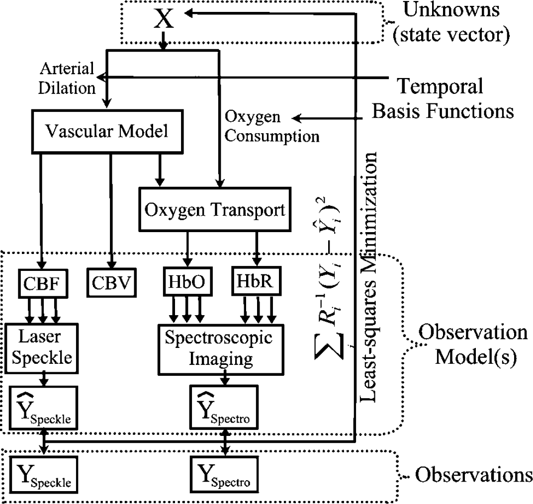
Schematic to the model framework: The proposed multicompartment model is based on a bottom-up approach to state/parameter estimation. A vector of unknowns (X) is used in a nonlinear through a set of differential equations describing the vascular and oxygen transport components of the hemodynamic response from a system input arterial dilation and oxygen consumption changes. The model outputs predict the changes in blood flow, volume, and oxygenation. These predictions are inputs into observation models, which describe measurement process for each measurement modality and are based on the biophysical principles governing each method. Multiple observation models create predictions of multimodality data, which are minimized to the experimental data using a pseudo-Bayesian fusion model, in the form of a weighted least-squares cost function.

Vascular Model

The vascular component of the model is described by a set of physical relationships that depict three connected, compliant, vascular compartments (namely the arterial, capillary, and venous compartments) and a constant volume compartment to model the pial venous structure (Table 1). The model of vascular changes described in this work is an extension of several previously proposed vascular models (reviewed in Buxton et al, 2004; Zheng et al, 2005). These models are built around the relationships between blood flow and volume changes originally proposed in the Balloon model (Buxton and Frank, 1997; Buxton et al, 1998) and later extended to include an empirical description of vascular compliance in the Windkessel model (Mandeville et al, 1999a, b ).

Table 1

Variables used in vascular model

Description	Symbol	Comments	Value	Citation
Resistance	R_n(t)	Resistance of nth compartment	Modeled-dynamic
	R _total	Total vascular resistance	1 (AU)
Capacitance	C_n(t)	Capacitance of nth compartment	Modeled-dynamic
	F_n,m(t)	Flow from compartment n –> m	Modeled-dynamic
Flow	F_in(t)	Flow into system	Modeled-dynamic
	F_out(t)	Flow out of system	Modeled-dynamic
	P_n(t)	Pressure of nth compartment	Modeled-dynamic
Pressure	P _in	Mean arterial blood pressure	1 (AU)
	P _out	Mean venous blood pressure	0 (AU)
	Φ_A	Baseline arterial volume fraction	25%
Volume Fraction	Φ_C	Baseline capillary volume fraction	15%	(Duong and Kim, 2000; Zheng et al, 2005)
	Φ_v	Baseline venous volume fraction	60%
Windkessel model	β	Windkessel vascular reserve	Modeled-static
	τ	Windkessel (vascular) transit time	Modeled-static

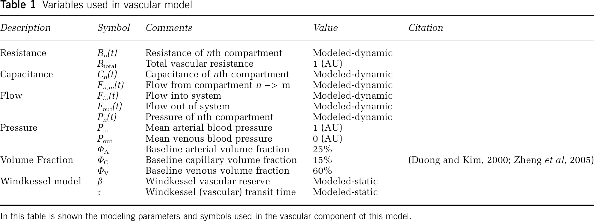
In this table is shown the modeling parameters and symbols used in the vascular component of this model.

The vascular compartments can be represented by an analogy to bridge a circuit of resistor and capacitor (electrical) elements as depicted in Figure 2 (Mandeville et al, 1999b). The resulting differential equations that govern changes in blood flow and volume are driven by the active dilation of the arteries, which decreases the input vascular resistance of the system. The pressure gradient between compartments (equivalent to electrical potential difference) drives the flow of blood (analogous to electrical current) between compartments. As the pressure increases, the vascular compartment expands causing blood volume to increase. The increase in blood volume in a compartment is equivalent to the build-up of charge on a nonlinear capacitor, whose capacitance decreases as the compartment expands against the pressure of the surrounding brain, leading to a saturating blood volume expansion function. Finally, the heart and systemic circulation create a constant pressure drop across the entire system and are modeled as a single constant DC voltage source.

Figure 2

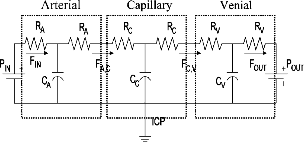
Schematic of the Windkessel vascular model: The Windkessel vascular model can be described based on an analogy to the electrical circuit shown here. Cerebral blood volume is equivalent to electrical charge. The flow of charge (i.e., current) models blood flow changes and is proportional to the blood pressure drop across compartments and inversely proportional to vascular resistance. Nonlinear capacitor elements model the vascular compliance of each compartment and the relationship between the cross-sectional area of a vascular segment and its vascular resistance.

The correspondence of this model with an electrical circuit readily allows the derivation of the differential equations to model the physical flow and volume changes based on Kirchoff's relationships and summarized by the following physical principles.

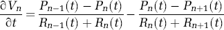
The flow between each compartment is calculated using the Ohm's law analogy (V = IR), where I, V, and R are analogous to the blood flow, blood pressure, and vascular resistance, respectively. The pressure (P) drop across vascular compartments (n → n + 1) is the product of the flow (F) from the nth into the (n + 1)th compartment and the vascular resistance (R) between the compartments,

P_{n} (t) - P_{n + 1} (t) = F_{n, n + 1} (t) [R_{n} (t) + R_{n + 1} (t)]

(1)

This leads to the set of differential equations that describe the differential volume changes in each compartment based on flow mismatch,

\frac{\partial V_{n}}{\partial t} = F_{n - 1, n} (t) - F_{n, n + 1} (t)

(2a)

\frac{\partial V_{n}}{\partial t} = \frac{P_{n - 1} (t) - P_{n} (t)}{R_{n - 1} (t) + R_{n} (t)} - \frac{P_{n} (t) - P_{n + 1} (t)}{R_{n} (t) + R_{n + 1} (t)}

(2b)

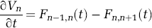
In this model, the capillary and venous compartments are compliant. The capacitance (C_n) describes the variable vascular compliance and hence the limit for volume changes in these compartments. In the electrical circuit analogy, charge build-up on these capacitors models blood volume changes. However, in the vascular network, compliance modeled by capacitance is a nonlinear function of the pressure (P_n) between the vascular compartment and the intracranial pressure and varies according to an inverse power law relation of Windkessel volume reserve (Mandeville et al, 1999b).

C_{n} (t) = A_{n} [P_{n} (t)]^{(1 / β_{n}) - 1} n \in {C a p i l l a r y, V e n o u s}

(3)

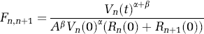
In this model, β_n is the Windkessel vascular reserve of the nth compartment. We assume the vascular reserve to have the same value for both the capillary and venous compartments. A_n is a scaling constant determined by the initial conditions,

A_{n} = V_{n} (0) / (F_{n - 1, n} (0) (R_{n - 1} (0) + R_{n} (0)))^{1 / β}

(4)

Combining equations (1)–(4), the flow in the capillary and venous compartments is a function of the pressure, volume, and the resistance of the compartments and is described by

F_{n - 1, n} = \frac{P_{n - 1} - V_{n} (t)^{β} / A^{β}}{R_{n - 1} (t) + R_{n} (t)}

(5a)

F_{n, n + 1} = \frac{V_{n} (t)^{α + β}}{A^{β} V_{n} (0)^{α} (R_{n} (0) + R_{n + 1} (0))}

(5b)

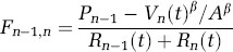
where α = 2 and represents laminar flow in the compartments (Mandeville et al, 1999b).

Volume expansion of the arteries is caused by the active dilation of these vessels. The changes in arterial volume (ΔV_A) are determined by the change in the diameter of the compartment (ΔD_A).

\frac{V_{A} (t)}{V_{A} (0)} = (\frac{D_{A} (t)}{D_{A} (0)})

(6)

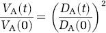
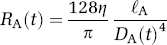
The arterial resistance (R_A) is proportional to the vessel's length (ℓ_A) and inversely proportional to the fourth power of its diameter (D_A) according to Poiseuille's Law (Washburn, 1921). η represents the viscosity of blood and is removed with normalization.

R_{A} (t) = \frac{128 η}{π} \frac{ℓ_{A}}{D_{A} (t)^{4}}

(7)

We sequentially apply differential temporal update to the arterial, capillary, and finally the venous compartment to calculate the blood flow and volume changes for each of the vascular compartments. This update is driven by changes in the arterial resistance, which is an input to the system and is described within the state vector. The value of the hydrostatic pressure of the subsequent compartment (i.e., capillary) at the previous time instance, and the vascular resistance and inflow to the present (i.e., arterial) compartment at the current time instant are used to calculate the differential update in the system. The same procedure is repeated to update the capillary and the venous compartments. The fourth compartment representing the pial veins is assumed to have constant blood volume and is defined by the flow and mean transit time (τ_pial) of the vascular segment. The mean transit time is determined by an additional parameter in the state model. The inclusion of a pial compartment was motivated by experimental observations outlining the role of these structures in the measurement of hemodynamic changes (Nielsen et al, 2000; Watanabe et al, 1994).

The differential equations (defined by equations (1)–(5)) can be formulated with variables of flow and resistance represented as unit-normalized quantities. Thus, the model naturally estimates relative changes in the hemodynamic parameters. In this work, we apply this model to data measurements by laser speckle and optical spectroscopic imaging. The laser speckle measurement is related to a relative change in blood flow, whereas spectroscopic measurements can approximate the absolute (i.e., micromolar) changes in oxy- and deoxy-hemoglobin concentrations. An additional state parameter, baseline total-hemoglobin (HbT_o), is used to scale the fractional changes in volume predicted by the model to the absolute concentration changes calculated from the optical measurements. This scaling factor has the physiologic interpretation of the total hemoglobin concentration in the imaging volume. Because this value is calculated from the functional data, this scaling factor encompasses errors in partial volume or optical path length that were not accounted for in the calculation of hemoglobin changes from the optical data.

At baseline, the relationship between the Windkessel volume and the incoming blood flow is given by the vascular transit time (V_w(0) = F_in(0)τ), where the Windkessel volume is equal to the sum of the volumes of the three-vascular compartments. We assume initial volume fractions of 25%, 15%, and 60% for the arterial, capillary, and venous compartments, respectively (Duong and Kim, 2000; Zheng et al, 2005). The sum of the initial total resistance in the three compartments is set at unity. The baseline arterial resistance (R_a(0)) is estimated by the state vector and the remaining resistance is equally distributed between the capillary and venous compartments (Boas et al, 2003).

Arterial Dilation

The arteriolar dilation variations that drive the flow and volume changes in the vascular network are defined in the state vector (X) and are estimated as part of the minimization of the residual model error with the hemodymanic measurements. We use a temporal Gaussian function to describe the response of arteriolar resistance during cerebral activation (Boas et al, 2003),

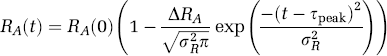
R_{A} (t) = R_{A} (0) (1 - \frac{Δ R_{A}}{\sqrt{σ_{R}^{2} π}} \exp (\frac{- (t - τ_{p e a k})^{2}}{σ_{R}^{2}}))

(8)

This function is defined by the baseline resistance (R_A(0)), the functional percent change in resistance (ΔR_A), the time-to-peak (τ_peak), and the temporal width (σ_R) of the response. These four parameters are estimated in the model as part of the state vector by the fitting procedure. The temporal basis function reduces the degrees of freedom of the arteriolar resistance by estimating a subset of state variables instead of the full dynamic variation and is similar to the use of temporal basis functions in the generalized linear model used in fMRI. As a future extension, this model could be improved with the inclusion of an explicit model of the release of vaso-reactive signaling molecules to model the response to measured neuronal stimulation (Riera et al, 2005).

Oxygen Transport Model

In addition to vascular effects, increased neuronal activity results in a localized increase in the mitochondrial function (Mintun et al, 2001) (Table 2). This increase results in elevated oxygen consumption. Cerebral metabolism increases the extraction of oxygen from the vascular network, whereas increased blood flow competes to lower the oxygen extraction fraction. Blood flow is usually the dominant factor that determines the overall blood oxygenation (i.e., deoxy-hemoglobin changes). The second element of our model describes the process of oxygen extraction from the vascular compartments. We introduce a model of the oxygen transport dynamics between the arterial, capillary, and venous compartments and the extravascular parenchyma tissue, which considers the differing permeability of these vessels. The oxygen extraction from all three compartments is based on recent experimental observations of such effects in animal models (Berwick et al, 2004; Tsai et al, 2003; Vovenko, 1999). The system is built on the principle of oxygen diffusion caused by the gradient of oxygen content between the vascular compartments and the extravascular tissue (c_nO₂ where n ∈ {arterial, capillary, venous, and tissue}) (Herman et al, 2006; Zheng et al, 2002). The vessels of the pial veins are assumed to negligibly contribute to oxygen delivery to the tissue and are only affected by the washout effects of increased flow.

Table 2

Variables used in oxygen transport model

Description	Symbol	Comments	Value	Citation
Partial pressure O₂	p_nO₂(t)	Partial pressure of O₂ in vascular segments or tissue	Modeled-dynamic
	p_inO₂	Mean incoming pO₂	100 mm Hg	(Herman et al, 2006)
	p_tissueO₂(0)	Baseline tissue pO₂	16 mm Hg
Oxygen saturation	S_nO₂(t)	Baseline {Art, Cap, Vein}	Modeled-static
Modeled-dynamic
Oxygen content	C_nO₂(t)	Baseline {Art, Cap, Vein, Tissue}	Modeled-static
Modeled-dynamic
Diffusivity rate constant	K_n	Oxygen permeability rate constant	Modeled-static
Cerebral metabolism	CMRO₂(t)	Metabolism temporal basis function	Modeled-static

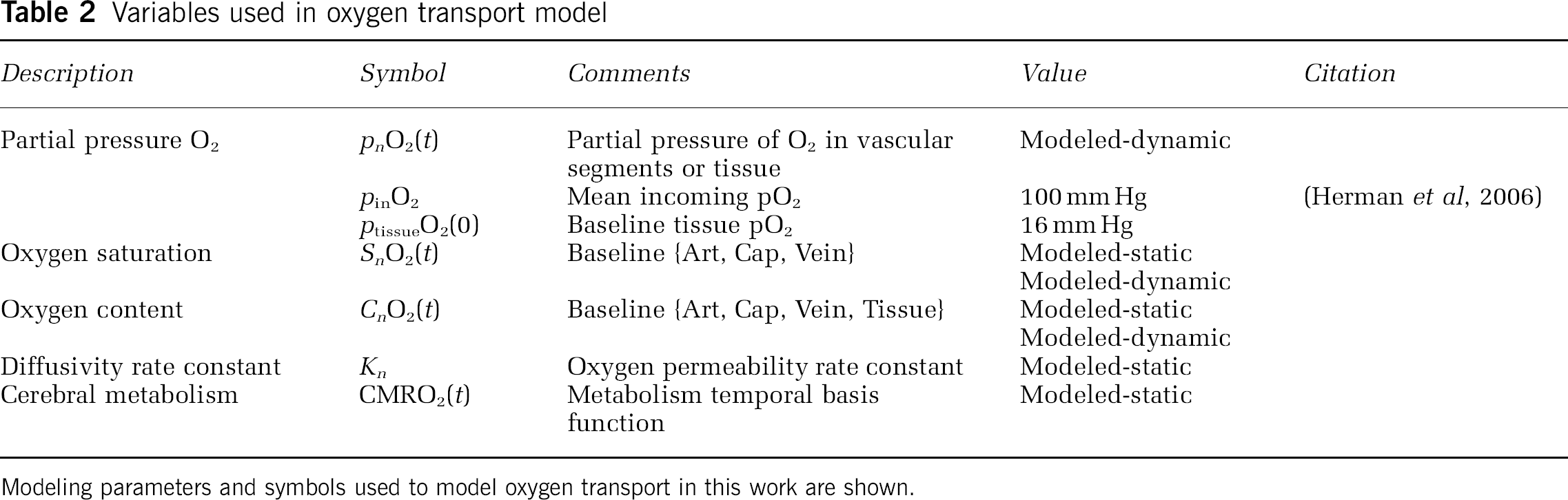
Modeling parameters and symbols used to model oxygen transport in this work are shown.

The oxygen content is the amount of oxygen carried within the blood and is the sum of the oxygen bound to hemoglobin and oxygen dissolved in the blood plasma (Habler and Messmer, 1997).

c_{n} O_{2} (t) = α_{p} p_{n} O_{2} (t) + H_{n} \cdot H G B \cdot S_{n} O_{2} (t)

(9)

The Hüfner number (H_n) is the amount of oxygen bound per gram of hemoglobin (H_n = 1.39 mL O₂/gm Hb (Habler and Messmer, 1997)). The hemoglobin content of blood (HGB) is assumed to be 16 gHb/dL of blood (Habler and Messmer, 1997). Finally, α_p is the solubility of oxygen in blood plasma (α_p = 0.0039 ml O₂/mm Hg dL (Habler and Messmer, 1997; Herman et al, 2006)). In the extravascular tissue, oxygen solubility is greater than in the plasma (α_t = 0.0118 mL O₂/mm Hg dL (Herman et al, 2006)). In the tissue, oxygen content depends only on oxygen partial pressure (i.e., c_tO₂(t) = α_t · p_tO₂(t)). Under normal physiologic conditions, the amount of plasma-dissolved oxygen in the blood offers a negligible contribution (~ 2% to 3%). However, including plasma oxygen allows this model to be generic enough to be used to model hyperoxic or hyperbaric conditions in future work.

To define oxygen transport between the vascular segments and the surrounding tissue, we derive a system of differential equations dependent on (i) the flow changes described by the vascular component of the model and (ii) changes in mitochondrial metabolism, which result in changes in oxygen consumption in the extravascular tissue compartment (Herman et al, 2006; Zheng et al, 2002).

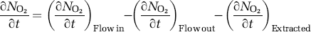
The changes in the oxygenation of each vascular compartment are functions of the amount of oxygen flowing into and out of the compartment and are governed by the blood flow and the oxygen extracted from the compartment to the surrounding extravascular tissue. Oxygen extraction is driven by the differences in the oxygen content between the vascular compartments and the surrounding tissue (Zheng et al, 2002, 2005),

\frac{\partial c_{N} O_{2} (t)}{\partial t} = - K_{N} [c_{N} O_{2} (t) - c_{T} O_{2} (t)]

(10)

where n ∈ {Arterial, Capillary, Venous} In equation (10), K_N is the intrinsic rate constant for this process and can be defined from the baseline relationships between SO₂, blood flow, and the pO₂ levels of the compartment and extravascular tissue. In this model, we include the effect of oxygen diffusion across both the arterial and venous walls, which has been suggested by experiential findings (Berwick et al, 2004; Vovenko, 1999).

To derive the equations for oxygen transport, we assume that all compartments obey the principles of mass balance of the amount of O₂ (N_O2), that is,

\frac{\partial N_{O_{2}}}{\partial t} = {(\frac{\partial N_{O_{2}}}{\partial t})}_{F l o w i n} - {(\frac{\partial N_{O_{2}}}{\partial t})}_{F l o w o u t} - {(\frac{\partial N_{O_{2}}}{\partial t})}_{E x t r a c t e d}

(11)

Using the relationship between the amount of oxygen carried in each compartment and the oxygen concentration $N_{O_{2}} (t) = c_{n} O_{2} (t) V_{n} (t)$ , we arrive at a set of differential equations for the delivery of oxygen into each of the vascular compartments,

\begin{aligned} \frac{\partial N_{O_{2}}}{\partial t} = & F_{I n} (t) \cdot c_{I n} O_{2} (t) - F_{o u t} (t) \cdot c_{o u t} O_{2} (t) \\ - K \cdot [\frac{1}{2} (c_{I n} O_{2} (t) + c_{O u t} O_{2} (t)) - c_{T} O_{2} (t)] \cdot V_{n} (t) \end{aligned}

(12)

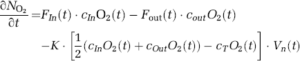
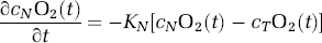
The mean oxygen content of a vascular segment has been defined as the average of the concentration (content) of either end (i.e., c_nO₂(t) = 1/2(c_InO₂(t) + c_OutO₂(t))). In the extravascular compartment, the change in the amount of oxygen is the difference between oxygen delivered to the tissue and oxygen consumed,

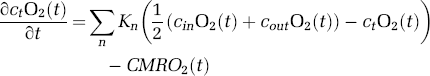
\begin{aligned} \frac{\partial c_{t} O_{2} (t)}{\partial t} = & \sum_{n} K_{n} (\frac{1}{2} (c_{i n} O_{2} (t) + c_{o u t} O_{2} (t)) - c_{t} O_{2} (t)) \\ - C M R O_{2} (t) \end{aligned}

(13)

The system of equations described by (12) and (13) can be solved using a discrete temporal update. The baseline CMRO₂ and rate constants (K_n) can be calculated from the baseline conditions, namely the baseline oxygen content in each compartment and the tissue is at steady state.

After solving for the oxygen content in each compartment, the oxygen saturation of hemoglobin and the partial pressure of oxygen dissolved in the plasma can be recovered with the nonlinear inversion of equation (9). The saturation of hemoglobin is also related to the partial pressure of oxygen by the hemoglobin dissociation curve described using Kelman's equation (Severinghaus, 1979) and can be used to derive temporal changes in the oxy- and deoxy-hemoglobin content in each compartment.

CMRO2

We use a modified version of the gamma variate function as a temporal basis function to describe functional changes in CMRO₂

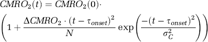
\begin{aligned} C M R O_{2} (t) = C M R O_{2} (0) \cdot \\ (1 + \frac{Δ C M R O_{2} \cdot (t - τ_{o n s e t})^{2}}{N} \exp (\frac{- (t - τ_{o n s e t})^{2}}{σ_{C}^{2}})) \end{aligned}

(14)

where CMRO₂(0) represents the baseline CMRO₂ in the mitochondria and ΔCMRO₂ represents the maximum percent change in CMRO₂ from its baseline value. τ_peak is the time to maximum change in CMRO₂ and σ_C is the temporal width of the response and N is a normalizing factor.

Measurement Models

The final component of this system is a model of the observation process depicted in Figure 1. We use module measurement model functions to describe the biophysics by which the auxiliary states (HbO₂, HbR, CBV, and CBF) are measured by the imaging modalities. Separating the measurement model allows us to readily extend this work to multimodality imaging measurements. In this work, we focus on the analysis of region-of-interest averages from laser speckle and optical spectroscopy. The measurement models are assumed to have uniform sensitivity to each compartment and these measurements represent the sum or the average of the contributions from all the vascular compartments (n ∈ {Arterial, Capillary, Venous, Pial vein}),

Y_{S p e c t r a l, H b X} (t) = \sum_{n} Δ H b X_{n} (t)

(15a)

Y_{S p e c k l e} (t) = \sum_{n} C B F_{n} (t) / \sum_{n} C B F_{o}

(15b)

The framework of this model allows the incorporation of true measurement sensitivity profiles, such as those obtained from the consideration of the optical photon transport process or fMRI measurement models. This could be extended to the fusion of multimodality data into image reconstructions of hemodynamic and metabolic changes and will be explored in future work.

Materials and methods

Experimental Methods

Animal preparation: The MGH Subcommittee on Research Animal Care approved all experimental procedures. Male Sprague—Dawley rats (250–350 g, n = 7) were anesthetized with 2% halothane and prepared as previously described in Dunn et al (2005). The skull over the somato-sensory cortex was thinned until transparent (approximately 100 μm). After surgery, anesthetic was switched to a 50 mg/kg bolus of α-choralose followed by continuous infusion at 40 mg/kg/h.

Stimulation protocol: A whisker deflection stimulus was used for stimulus as described in Devor et al (2003). The stimulus consisted of a single whisker deflection of varying amplitude (from 1 to 9) and 20 ms duration. The angular velocity increased from 203°/s (vertical displacement of 240 μm, condition 1) to 969°/s (vertical displacement of 1200 μm, condition 9), with equal amplitude increments. Stimuli were presented using a rapid, randomized event-related paradigm.

Description of optical spectroscopy system and analysis: Multi-wavelength spectroscopic imaging of total hemoglobin concentration and oxygenation were performed using the instrument and methods described in Dunn et al (2005). Briefly, the cortex was illuminated by a filtered mercury xenon arc lamp (10-nm band pass filters centered at wavelengths of 560, 570, 580, 590, 600, and 610 nm). Images were acquired onto a cooled 12-bit CCD camera at a frame rate of 18 Hz. The modified Beer—Lambert law was used to convert these spectral images into images of oxy- and deoxy-hemoglobin concentration changes. Differential path-length factors were used to account for the individual optical path lengths at each wavelength (Kohl et al, 2000).

Description of laser speckle system and analysis: Blood flow was imaged using laser speckle contrast by the method and instrument described in Dunn et al (2005). Images of relative CBF changes were determined by calculating the changes in the speckle contrast in a series of laser speckle images. The speckle contrast is calculated as the ratio of the standard deviation to the mean pixel intensities, 〈I²-〈I〉² 〉 ^0.5/〈I〉 over a 7 × 7 pixel sliding window (Briers, 2001). Speckle contrast images were averaged across trials and the averaged set was converted to relative blood flow (1 + ΔCBF/CBF_o) by converting each speckle contrast value to an intensity autocorrelation decay time (Briers, 2001) and dividing by baseline (Dunn et al, 2005).

Determination of hemodynamic response: Both laser speckle and spectroscopic results were deconvolved using the stimulus presentation timing to determine the blood flow and hemoglobin responses. Colocalized regions-of-interest were manually selected and averaged for each experimental run of all animals. The group average of the seven animals was calculated after normalizing to the amplitude of the ninth condition. The measurement error was computed from the variance of the data compared with the average of the seven rats.

Model parameters and initial conditions: We use a nonlinear, Levenberg—Marquardt algorithm implemented in Matlab (Marquardt, 1963) to estimate the states that describe the CMRO₂ and arterial dilation functions. A differential time step of 2 ms was used for the update of the vascular and oxygen transport models. Smaller time steps were also tested to verify that the results were independent of this choice. Multimodality measurements were integrated using a weighted least-squares cost function, where the weights were determined by the inverse of the measurement variances for each modality as depicted in Figure 1. These weights were calculated from the variance in the estimate of the hemodynamic responses across the seven rats (Table 3).

Table 3

State variables

	Symbol	Description	Physiological range	Citation
Dynamic
Arterial dilation temporal basis	ΔR_A	Change arterial resistance	(0–10) %	—
	τ_peak	Time to maximum resistance change	(0–6) s	—
	σ_A	Width of temporal resistance change	(0–6) s	—
	ΔCMRO₂	Relative change CMRO₂	(0–10) %	—
CMRO₂ temporal basis	τ_onset	Time to onset of CMRO₂ change	(0–6) s	—
	σ_c	Width of temporal CMRO₂ change	(0–6) s	—
Structural
Resistance	R_A(0)	Initial arterial resistance	(0.20–0.90) AU	(Mandeville et al, 1999b; Boas et al, 2003)
Windkessel parameters	β	Windkessel vascular reserve	(1–5) AU	(Mandeville et al, 1999b; Boas et al, 2003; Zheng et al 2005)
	τ	Vascular transit time	(0.5–4) s	(Mandeville et al, 1999b; Zheng et al, 2002; Boas et al, 2003)
	τ_pial	Pial venous transit time	(0–4) s	—
Baseline volume	[HbT]₀	Total baseline hemoglobin	(40–140) μmol/L	(Zheng et al, 2005; Boas et al, 2003)
	S_aO₂	Baseline arterial saturation	(95–100) %
Oxygen saturation	S_cO₂	Baseline capillary saturation	(60–90) %^a	(Herman et al, 2006)
	S_vO₂	Baseline venous saturation	(55–89) %^a

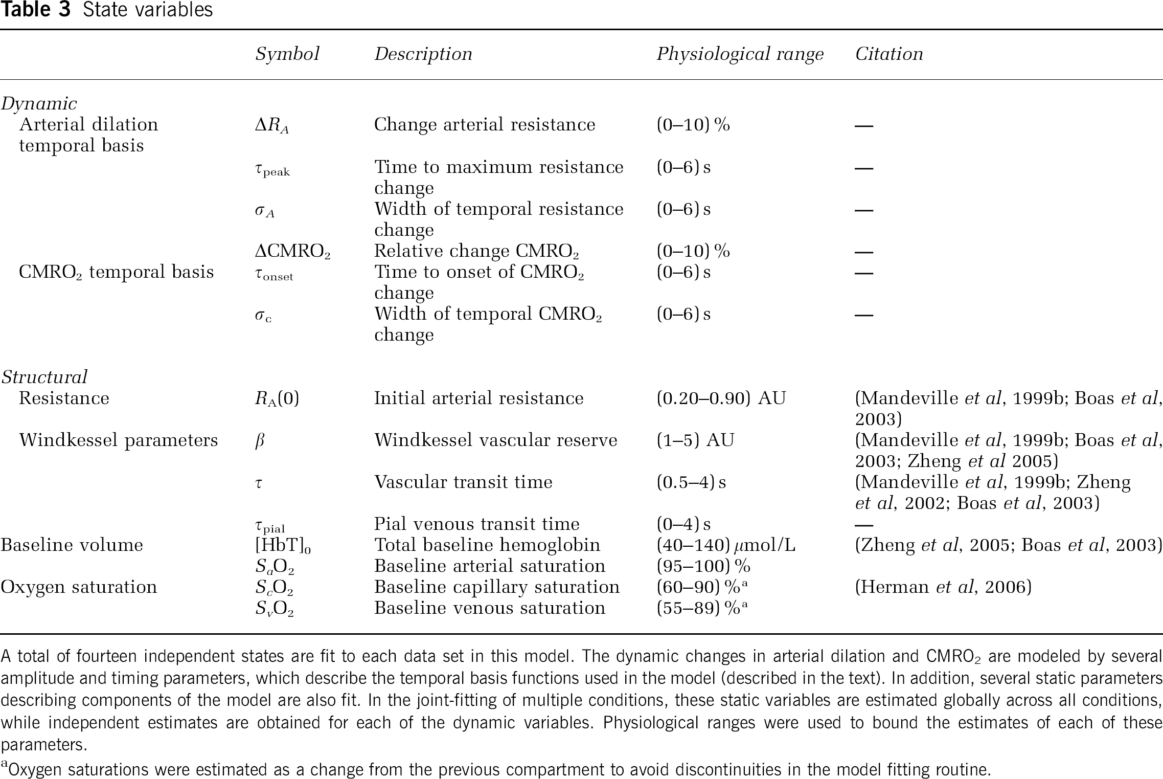
A total of fourteen independent states are fit to each data set in this model. The dynamic changes in arterial dilation and CMRO₂ are modeled by several amplitude and timing parameters, which describe the temporal basis functions used in the model (described in the text). In addition, several static parameters describing components of the model are also fit. In the joint-fitting of multiple conditions, these static variables are estimated globally across all conditions, while independent estimates are obtained for each of the dynamic variables. Physiological ranges were used to bound the estimates of each of these parameters.

Oxygen saturations were estimated as a change from the previous compartment to avoid discontinuities in the model fitting routine.

In Table 4, we summarize the model parameters estimated in the minimization process. The physiologic range of values for each parameter was used to impose a constraint on the upper and lower bounds of fitting values. The fitting routine was iterated until a defined convergence criterion (10⁻⁶ times the variance of the measurement error) was met. Each of the nine stimulus conditions was independently fit and the process took approximately 120 mins per condition (Pentium(R) 4; 3.0 GHz). We verified that the final estimate was independent of the choice of the initial guess for each state and the same initial guess was used for each of the nine conditions.

To estimate the confidence-bounds for each of the model parameters, we performed a Markov Chain Monte Carlo sampling of the state-space (Carter and Kohn, 1996). We used the change in χ² value at each sample step to approximate ʻenergy cost' to determine the probability of the acceptance of each step using the equation,

P (k | {j \leq k}) = [1 i f Δ χ^{2} \leq 1 e^{- Δ χ^{2}} e l s e],

(16)

where k defines the index current iteration and {j < k} is the set of all previous steps. The density of samples approximates the nth-dimensional probability density function, where n is the number of degrees-of-freedom of the state-vector. This defines the confidence bounds on each of the estimated parameters.

Table 4

State estimates

	Variable	Stimulus condition									Mean	Fit together
		1	2	3	4	5	6	7	8	9
Dynamic
Arterial dilation temporal basis	ΔR_A	0.94	1.05	1.41	1.72	1.69	1.84	2.57	2.65	3.00	*	—
	τ_peak	3.00	3.11	2.96	3.12	3.11	3.03	3.32	3.26	3.22	*	—
	σ_A	2.38	1.97	1.35	1.15	1.48	1.32	1.55	1.56	1.36	—	—
CMRO₂ temporal basis	ΔCMRO₂	0.53	0.24	0.34	0.35	0.22	0.27	1.28	0.36	0.28	—	—
	τ_peak	1.49	1.86	1.68	1.49	1.71	1.91	1.32	1.37	1.27	—	—
	σ_c	1.77	1.15	1.11	1.72	1.61	1.54	2.12	1.84	1.08	—	—
Structural
Resistance	R_A(0)	0.73	0.77	0.74	0.73	0.76	0.77	0.66	0.68	0.76	0.73	0.79
	β	1.32	1.33	2.27	2.79	1.21	1.14	2.94	1.52	1.19	1.75	1.45
Windkessel parameters	τ	0.79	0.68	0.65	1.31	0.70	0.66	0.75	0.62	0.61	0.75	0.60
	τ_pial	1.27	0.77	0.75	1.09	0.59	0.71	1.40	0.80	0.63	0.89	0.96
Baseline volume	[HbTJ₀	113.8	118.7	114.3	133.4	112.9	110.7	133.4	92.4	87.7	113.04	102.5
	S_aO₂	0.940	0.940	0.950	0.972	0.947	0.943	0.973	0.939	0.938	0.95	0.938
Oxygen saturation	S_cO₂	0.709	0.704	0.731	0.749	0.740	0.712	0.732	0.730	0.747	0.73	0.694
	S_vO₂	0.635	0.631	0.656	0.687	0.667	0.635	0.655	0.656	0.673	0.66	0.616

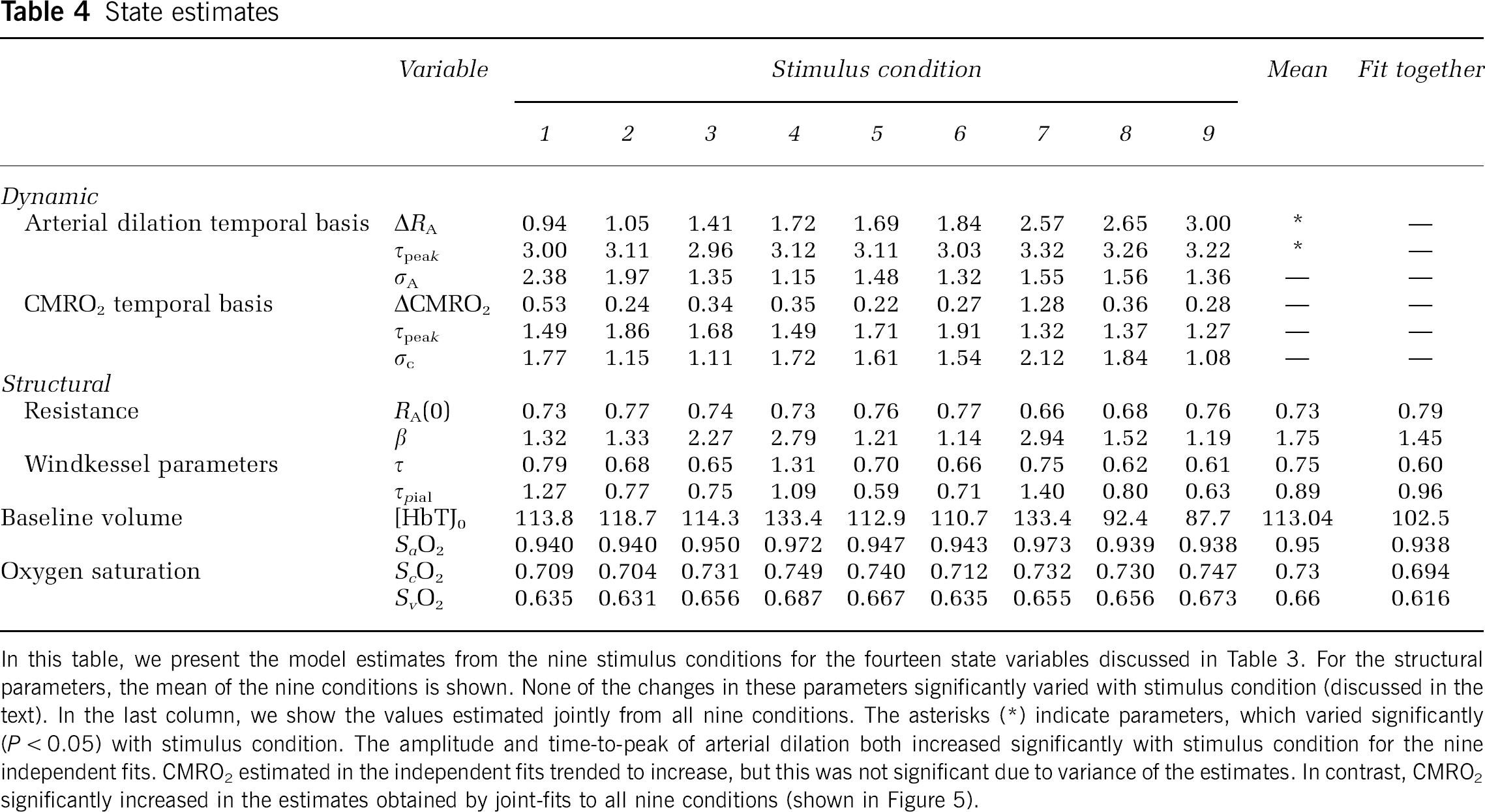
In this table, we present the model estimates from the nine stimulus conditions for the fourteen state variables discussed in Table 3. For the structural parameters, the mean of the nine conditions is shown. None of the changes in these parameters significantly varied with stimulus condition (discussed in the text). In the last column, we show the values estimated jointly from all nine conditions. The asterisks (*) indicate parameters, which varied significantly (P < 0.05) with stimulus condition. The amplitude and time-to-peak of arterial dilation both increased significantly with stimulus condition for the nine independent fits. CMRO₂ estimated in the independent fits trended to increase, but this was not significant due to variance of the estimates. In contrast, CMRO₂ significantly increased in the estimates obtained by joint-fits to all nine conditions (shown in Figure 5).

Single-compartment Windkessel model: We compare results from the proposed multicompartment vascular model with the previously published, single-compartment version of the Windkessel model (Mandeville et al, 1999b; Boas et al, 2003) using a similar fitting procedure. A single-compartment simplification of the current model was constructed from a dilating artery and a single compliant (Windkessel) compartment (Mandeville et al, 1999b). In our construction of the single-compartment model, we follow the same model framework as used in our multicompartment model and diagramed in Figure 1. We used temporal basis functions to describe the arterial dilation and CMRO₂ time courses while performing a nonlinear minimization to estimate the unknown states. This inductive modeling approach is similar to fitting of arterial dilation described in Boas et al (2003), but represents a significant deviation from the deductive approaches used in most other similar model descriptions (Zheng et al, 2002). This allows us to infer arterial dilation and CMRO₂ from the joint set of measurements within the same pseudo-Bayesian framework used in the multiple compartment model and thus make direct comparisons of the results.

The single-compartment model had 11 degrees-of-freedom (refer to Table 3), where the pial transit time was eliminated and the capillary and venous oxygen saturations were reduced to a single compartment. The bounded ranges for all parameters were the same as the multicompartment model in agreement with the previous literature (Boas et al, 2003). The baseline vascular fractions were assumed to be 25% and 75% for the arterial and Windkessel compartments, respectively.

Calculating baseline parameters: A unique feature of this model is that the concentration of baseline total hemoglobin is fit from the scale between the percent-change predictions of the model and the micromolar measured changes in hemoglobin concentrations calculated from the spectroscopic optical data. This value sets the scale for the entire model. This allows the value of baseline blood flow to be calculated from the equation,

C B F_{o} = H b T_{o} / (τ H G B)

(17)

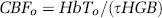
The vascular transit time (τ) is also estimated as part of the model. HGB is the hemoglobin content of blood, assumed to be 16 g Hb/dL (Habler and Messmer, 1997). Note that if HGB is unknown, we can still estimate hemoglobin flow (g Hb/sec).

Oxygen delivery is the product of the incoming flow of blood and oxygen content of the blood (defined in equation (9)). The partial pressure of oxygen in incoming arterial blood was assumed to be 100 mm Hg (Herman et al, 2006), which equates to an oxygen saturation of 98.7% (Severinghaus, 1979). Similarly, at baseline steady state, CMRO₂ is the product of blood flow and the oxygen extraction fraction across the compartments (OEF = (s_inO₂–s_outO₂)/s_inO₂). The drops in oxygen content across each vascular compartment are defined by parameters fit in this model and are determined by the baseline oxygen saturation of each compartment.

Results

Multicompartment Estimates

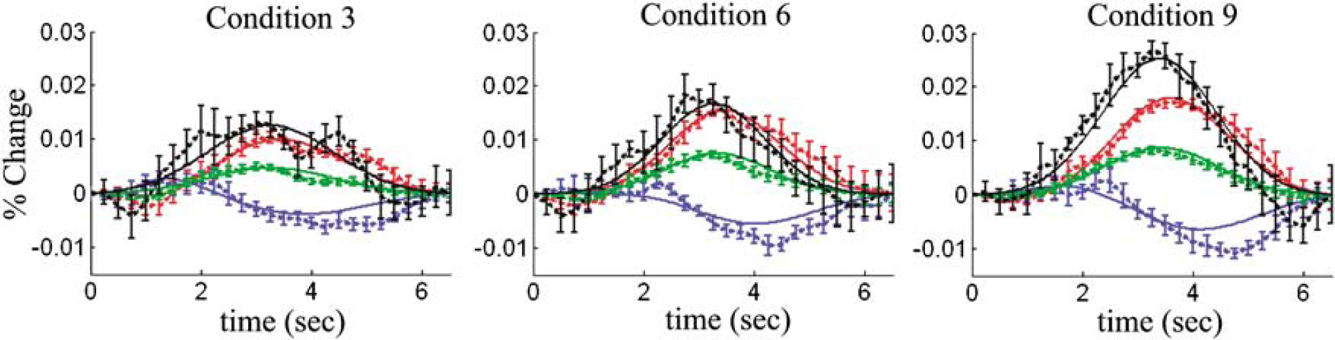
The unknown state parameters listed in Table 3 were estimated using the multicompartment model to fit the region-of-interest averaged response of the seven rats. The response curves from each of the nine conditions were fit independently and state estimates for each of these nine stimulus amplitudes are provided in Table 4 and the model fits to the experimental data for (representative) conditions 3, 6, and 9 as shown in Figure 3. The fits modeled nearly all the variance of the response for the hemodynamic parameters and yielded highly significant R² fits to each of the nine conditions, as summarized in Table 5. The partial R² values (adjusted for the model degrees-of-freedom) were calculated from the variance of the individual hemodynamic measurements (HbO₂, HbR, total-HB, and/or CBF) and the model results. This allowed us to examine the goodness-of-fit for each of the multimodal observations. The calculation showed nearly equally distributed variances across each of the measurements and showed that the model equally incorporated each of the measured components.

Figure 3

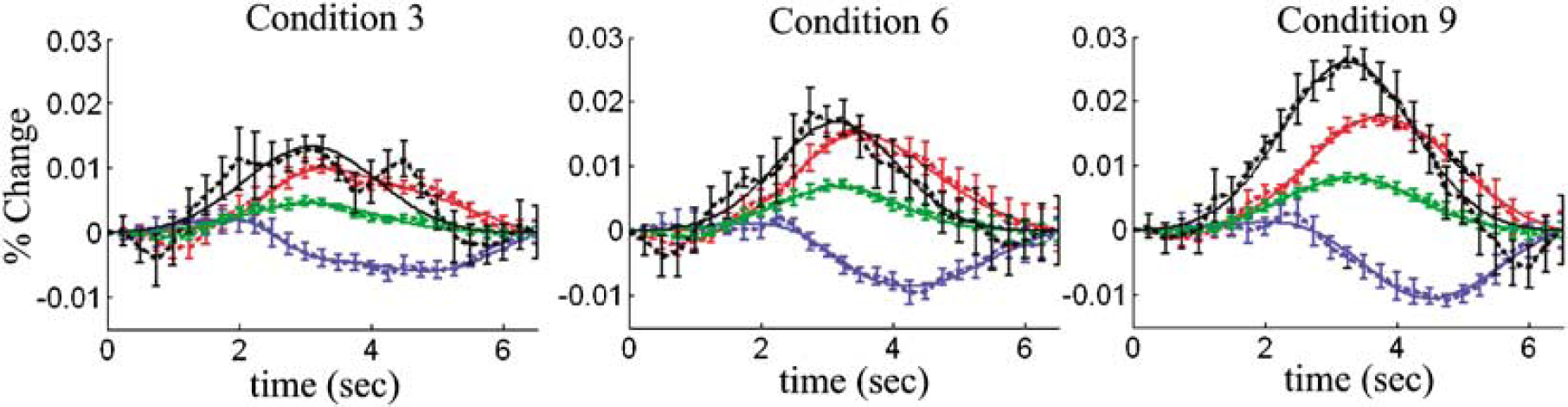
Multicompartment model fit to the experimental data: the experimental data (dotted lines) was fit using the multicompartment model (solid lines). Here we show representative results from the model fits to stimulus conditions 3, 6, and 9. The error bars show standard error estimated from the seven rats used in this experiment. Each condition was fit independently to generate these plots. The R² values for these fits are shown in Table 5. Blood flow (black) was measured by laser speckle imaging (Dunn et al, 2005). Total-, oxy- and deoxy-hemoglobin changes (green/red/blue) were calculated from measurements by optical spectroscopy (Dunn et al, 2005).

The state parameters estimated by this model consist of both structural and functional properties of the system. The parameters characterizing the functional response (CMRO₂ and arterial dilation) are expected to differ between the stimulus conditions, whereas the structural estimates are expected to remain constant. To test this hypothesis, we grouped the results of conditions 1 to 3, 4 to 6, and 7 to 9 and performed a one-way analysis of variance (ANOVA) test between groups. As expected, the estimates of the functional states varied significantly (P < 0.05) across the three groups, as indicated with an asterisk in Table 4. We found that magnitude and time-to-peak of the estimated arterial dilation and CMRO₂ responses increased with stimulus condition. These estimates are shown in Figure 4. In contrast, the estimate for the structural parameters did not vary significantly across the three groups. For these parameters, the mean of the nine conditions is shown in Table 4. The Windkessel vascular reserve (β) was estimated in the range of 1.1 to 2.9 (mean 1.8) for all nine conditions. Similarly, the estimate of the vascular transit time (τ) was also conserved across the three groups of conditions with a range of 0.61 to 1.31 secs (mean 0.70 secs). In addition, we estimated baseline total-hemoglobin to be 88 to 133 μmol/L (mean 113 μmol/L).

Figure 4

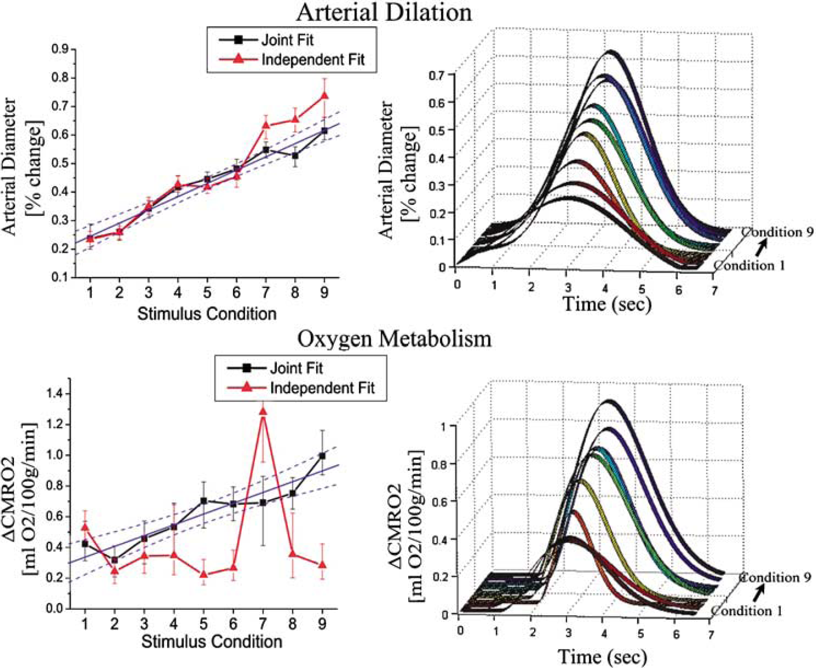
Parametric estimates in CMRO₂ and arterial dilation changes: The multicompartment model estimated parametric increases in both arterial dilation and CMRO₂ changes over the nine stimulus amplitudes. In the plots on the left, we show the parametric changes in the diameter of the arterial vessels (expressed as a percent change) and CMRO₂ (expressed in mL O₂/100 g min as described in the text). The temporal basis functions estimated from the model fits to the nine conditions (fit jointly) are shown in the figures on the right, where the evoked response lasted from 1.5 to 6 secs. The results of both the independent (red lines-triangle) and joint (black lines-square) model fits of the nine conditions were consistent. However, the joint estimates had lower variance than the independent fits for both estimates. The changes in both CMRO₂ and arterial diameter were linear with the stimulus condition (R² = 0.87 and 0.96, respectively). The blue lines show the linear fit to the estimates from the joint fitting, with 95% confidence bounds.

Table 5

Single- and multi-compartment model fits to experimental data

	Stimulus condition
	1	2	3	4	5	6	7	8	9
Multi-compartment
R²_adj–HbO₂	0.94	0.98	0.97	0.90	0.99	0.98	0.98	0.99	0.99
HbR	0.81	0.98	0.98	0.95	0.96	0.98	0.97	0.99	0.98
HbT	0.94	0.96	0.93	0.87	0.99	0.97	0.98	0.99	0.99
CBF	0.92	0.73	0.86	0.92	0.99	0.96	0.98	0.92	0.97
Total	0.91	0.95	0.95	0.89	0.98	0.98	0.98	0.98	0.99
Single-compartment
R²_adj–HbO₂	0.94	0.96	0.93	0.85	0.98	0.97	0.95	0.98	0.98
HbR	0.62	0.81	0.66	0.68	0.81	0.79	0.76	0.81	0.74
HbT	0.94	0.95	0.90	0.87	0.98	0.95	0.97	0.98	0.98
CBF	0.93	0.63	0.85	0.92	0.97	0.93	0.98	0.88	0.95
Total	0.89	0.88	0.87	0.87	0.95	0.93	0.94	0.95	0.95

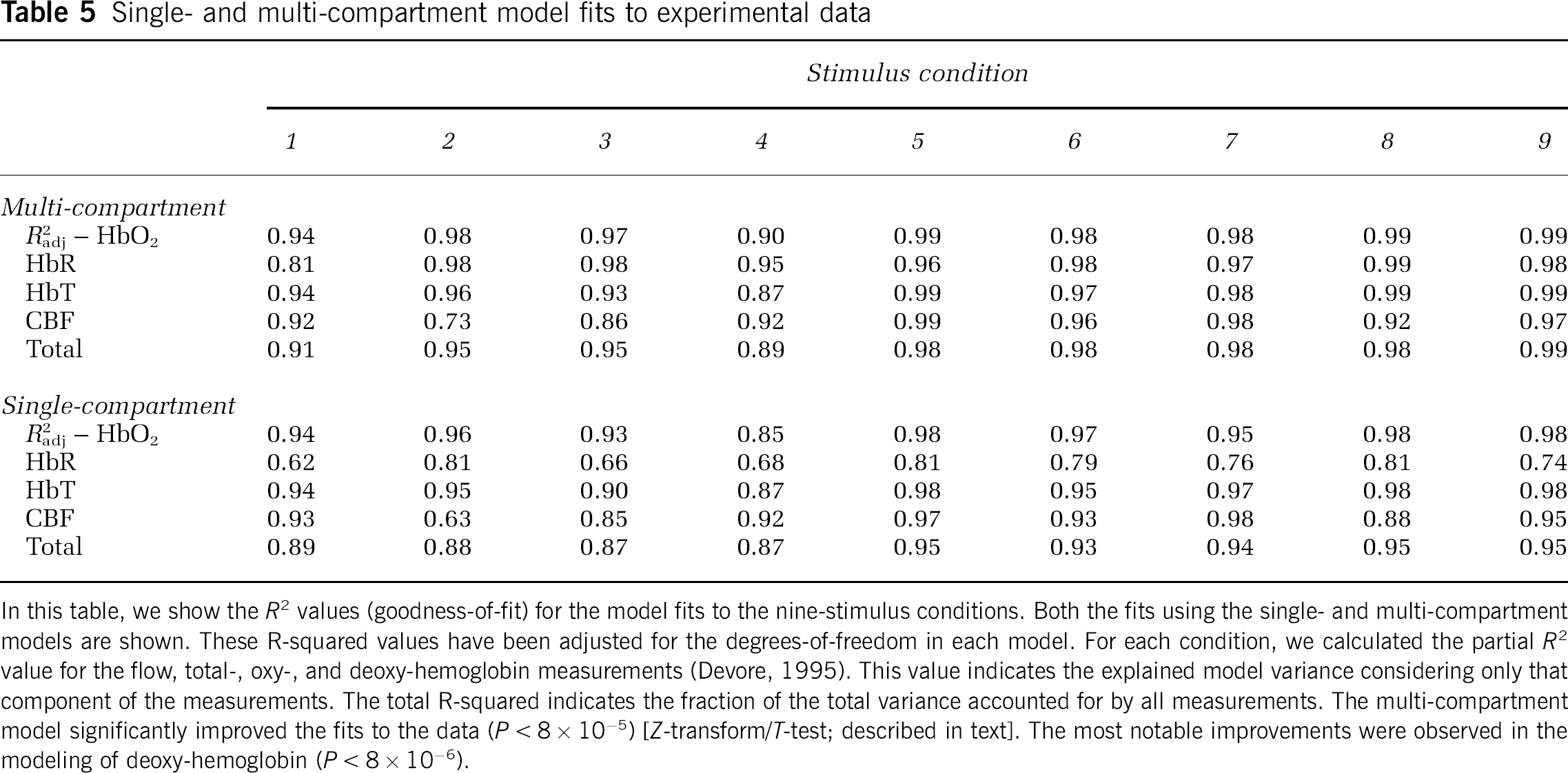
In this table, we show the R² values (goodness-of-fit) for the model fits to the nine-stimulus conditions. Both the fits using the single- and multi-compartment models are shown. These R-squared values have been adjusted for the degrees-of-freedom in each model. For each condition, we calculated the partial R² value for the flow, total-, oxy-, and deoxy-hemoglobin measurements (Devore, 1995). This value indicates the explained model variance considering only that component of the measurements. The total R-squared indicates the fraction of the total variance accounted for by all measurements. The multi-compartment model significantly improved the fits to the data (P < 8 × 10⁻⁵) [Z-transform/T-test; described in text]. The most notable improvements were observed in the modeling of deoxy-hemoglobin (P < 8 × 10⁻⁶).

To examine the influence of the choice of temporal basis functions used to model arterial dilation and CMRO₂, we examined other combinations of symmetric (Gaussian: equations (8)) and asymmetric (modified Gamma function: equations (14)) functional forms. No parameters except for the offset time (τ_onset or τ_peak) and temporal width (σ) varied significantly (P < 0.05: two-way ANOVA). In addition, all four combinations gave equal goodness-of-fit values (R²) for all individual measurements and the overall model (P < 0.05; Z-transform T-test). The models dependence on the initial seed of the Levenberg—Marquardt algorithm was also tested. Results did not significantly vary (P < 0.05: two-way ANOVA) (shown in Figure 5C).

Figure 5

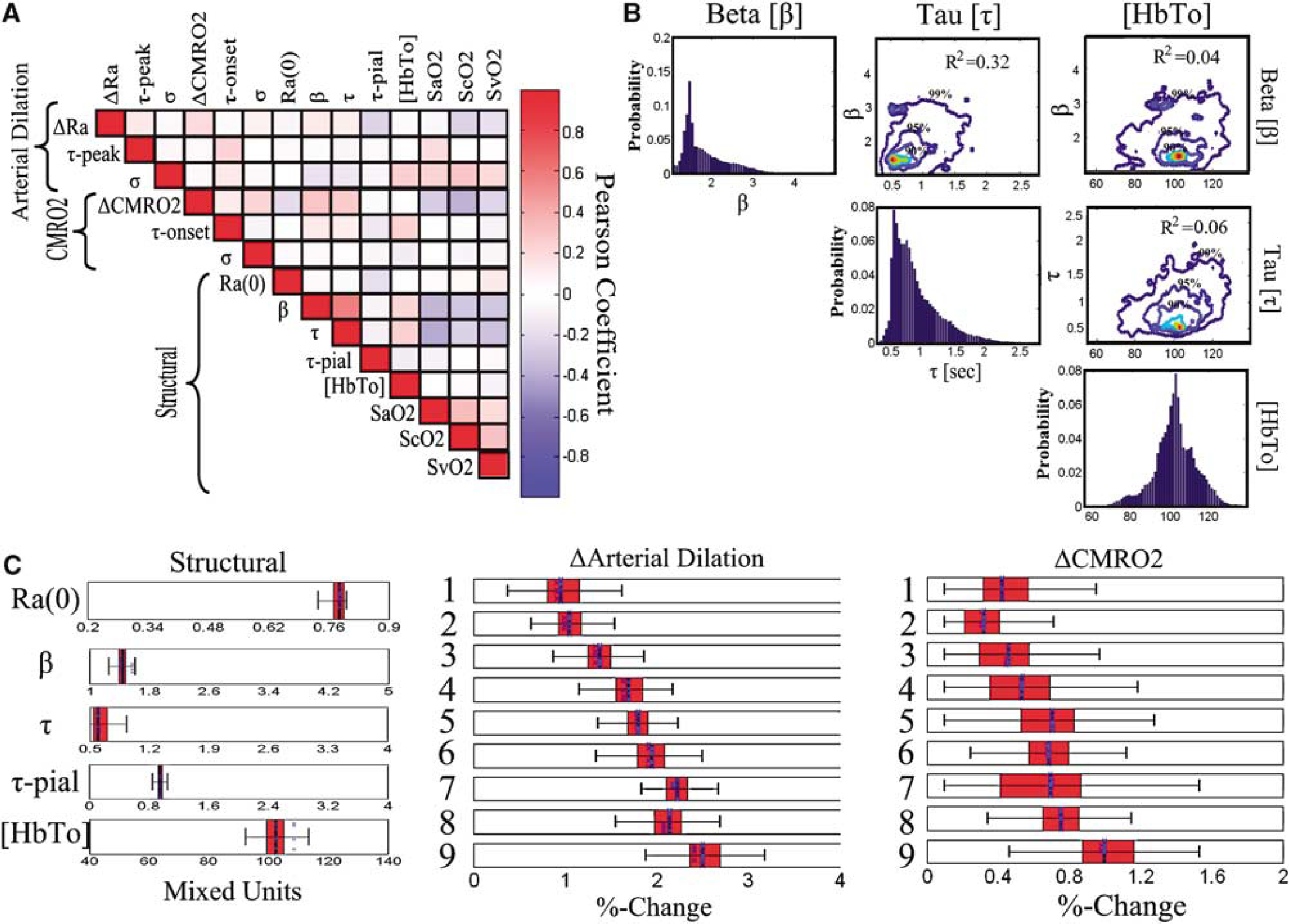
Markov chain Monte Carlo results: We used Markov chain Monte Carlo techniques to examine the variance in the estimates of each state fit by the model and the independence of these estimate (Carter and Kohn, 1996). In subplot (A), we show a correlation matrix formed from the pair-wise correlation of the uncertainties in the state variables. High correlation indicates interdependence between two variables, which could indicate crosstalk between these parameters in the model. In subplot (B), we show probability densities for three of the structural parameters (β, τ, and [HbT_o]). The histograms (diagonal element subplots) show the probability densities projected through all other degrees-of-freedom and indicate the error in the estimate (i.e., width of peak). The contour plots are created by the cross-section of this probability density along the two degrees-of-freedom in the plot (i.e., the correlation between β and [HbT_o] top right image). These cross-sections indicate the interdependence of these two variables by showing the correlation between them. Contour lines are indicated at the 99%, 95%, and 90% boundaries. In subplot (C), we show the mean and uncertainties in the parameter estimates fit to the nine conditions simultaneously. The model fits were repeated for 50 iterations of uniformly sampled initial positions for the Levenberg—Marquardt algorithm. The final minimization values are shown as scatter points for each parameter. Irregardless of starting position, all final estimates fell within the model uncertainty of each parameter.

Joint Estimates Using all Stimulus Conditions

After fitting the nine stimulus conditions independently and noting the constancy of the structural parameters, we concatenated the state-vectors such that the model independently estimated the arterial dilation and CMRO₂ functions for each condition, but used common estimates for the structural and static variables. This procedure was used to reduce the degrees-of-freedom of the model and simultaneously incorporate data from all nine conditions, thus giving a better estimate of the arterial dilation and CMRO₂ responses. The structural parameters from this fit were consistent with the average values obtained from the independent fits (see Table 4).

The arterial dilation and CMRO₂ changes estimated using all nine conditions are shown in Figure 4. The variance in these estimates was reduced as compared with the results obtained by independently fitting each condition. The solid lines shown in Figure 4 show the linear fits through the estimates from the simultaneous fitting of all nine conditions. The arterial dilation response increased linearly with stimulus amplitude (R² = 0.96). Similarly, the CMRO₂ change increased linearly with stimulus amplitude (R² = 0.87).

Model Uniqueness

To examine the uniqueness of the model fits, we examined the results using Markov chain Monte Carlo simulations to estimate the variance in each of the estimates. This approach was followed to examine underlying connections between the individual states and their estimates. In Figure 5, we show the correlation of the error in the state estimates for the joint-fitting of all nine conditions. In such an image, a high degree of correlation would indicate interdependence between two (or more) state variables. Instead, we observe low correlation between most of these individual state estimates, which indicates that these states were fairly independently estimated. Only a few of these correlations met a significance criterion (P < 0.05). First, a minor positive correlation was observed between the estimates of the Windkessel vascular reserve (β) and transit time (τ) (R² = 0.32). In addition, we noted a slight negative correlation between the baseline SO₂ for the three compartments and fractional change in CMRO₂ (R² = 0.07, 0.13, 0.05; S_aO₂, S_cO₂, S_vO₂). A similar negative correlation was observed between the uncertainty in the estimate of the Windkessel vascular reserve and transit time and SO₂. This result is not surprising since baseline SO₂ and transit time determine baseline CMRO₂. To further examine the state estimates of the Windkessel vascular reserve (β), transit time (τ), and baseline total hemoglobin ([HbT_o]), in Figure 5B, we show the cross-section through the probability distribution clouds along these degrees-of-freedom. Contour lines are shown at the 99%, 95%, and 90% boundaries. In these plots, correlation between these variables would manifest as alignment along the diagonals of the plots. The largest correlation was observed between vascular reserve and transit time. The histograms for the projection along the axis of each degree-of-freedom yield the confidence bounds for each of the states.

Comparison to the Single-Compartment Windkessel Model

To further examine the validity of the proposed multiple compartment model, we compared our results with those from the previously described single-compartment Windkessel models (Boas et al, 2003; Mandeville et al, 1999b). We found that the shortcomings of single-compartment Windkessel model were primarily seen in the fits of the oxygenation component of the hemodynamic response to the experimental data (shown in Figure 6). This result is in agreement with the similar findings by Zheng et al (2005) of a multicompartment model. The degree-of-freedom adjusted R² and partial R² values for both the multicompartment and single Windkessel-compartment model fits are shown in Table 5. Using a Z-transform, we performed a paired T-test of these fits (Devore, 1995). We found that the single Windkessel-compartment model had significantly worse agreement for the deoxy-hemoglobin (P < 8 × 10–⁶) and oxy-hemoglobin (P < 2 × 10⁻⁴) time courses. The blood flow and volume estimates were also significantly better in the multicompartment model by this test (P < 6 × 10⁻³ and P < 2 × 10⁻³). The overall model fit to all observations was also significantly better for the multicompartment model (P < 8× 10⁻⁵).

Figure 6

Single-compartment model fit to the experimental data: The experimental data (dotted lines) was fit using the single-compartment model (solid lines). Here we show representative results from the model fits to stimulus conditions 3, 6, and 9. Each condition was fit independently to generate these plots. The R² values for these fits are shown in Table 5. Blood flow, and total-, oxy- and deoxy-hemoglobin changes are shown in black, green, red, and blue, respectively. The error bars represented standard errors estimated from the seven rats used in this experiment.

The estimates of arterial dilation and CMRO₂ are shown in Figure 7. We found that the estimates of CMRO₂ and the errors in the estimates are significantly higher for the single compartment than for the multiple compartment model. This is in agreement with findings reported previously (Zheng et al, 2005).

Figure 7

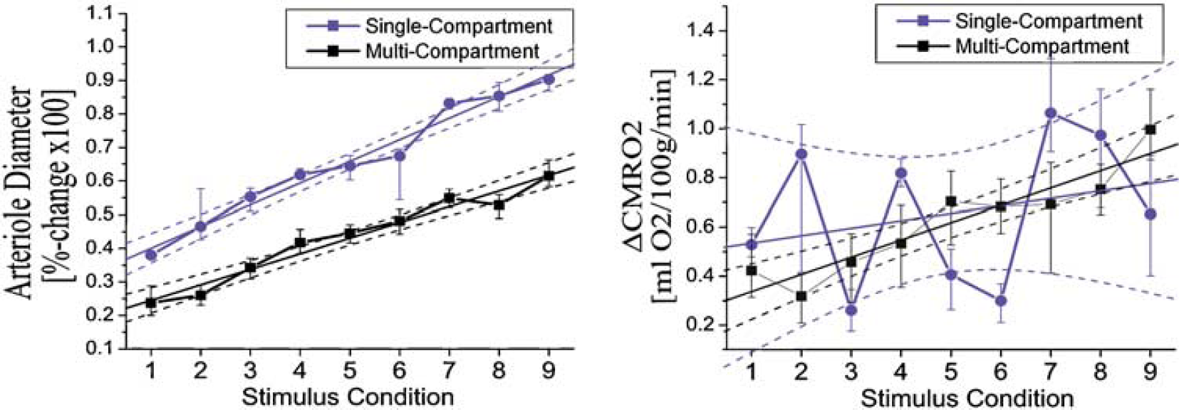
Comparison of CMRO₂ and arterial dilation changes from single- and multi-compartment models: In these two plots, we show the parametric changes in arterial diameter (left) and CMRO₂ (right) estimated by the single-compartment (blue line; circle) and multicompartment (black line; square) models. Both estimates are from the joint-fitting of the nine conditions. In both models, arterial diameter changes were linear with stimulus amplitude (R² = 0.98 (single) and R² = 0.96 (multi)). The single-compartment estimates were significantly greater than the multi-compartment estimates (P < 2 × 10⁻⁶) (paired T-test). CMRO₂ changes estimated with the multicompartment model were linear (R² = 0.87) with stimulus condition. The single-compartment estimates were more variable (R² = 0.08). Owing to this variance, the difference in the two model estimates was not significant.

Estimated Baseline Properties

Our model allows the estimation of the vascular transit time, baseline oxygenations, and the absolute baseline hemoglobin concentration. These can be used to estimate baseline blood flow and oxygen consumption from the initial relationship between the initial Windkessel volume and incoming blood flow (V_w(0) = F_in(0) · τ). At baseline, we can assume steady-state conditions and relative CMRO₂ can be calculated directly from the baseline blood flow and oxygen extraction fraction (OEF) (i.e., rCMRO₂(0) = F_in(0)OEF). The estimates of these baseline properties are shown in Table 6. From the mean of the nine stimulus conditions, we estimate baseline blood flow to be 94 ± 15 mL/100 g min using an assumed hemoglobin content (HGB) of 16 g/dL (Habler and Messmer, 1997). From the oxygen carrying capacity of oxy-hemoglobin (H_n = 1.39 mL O₂/gHb (Habler and Messmer, 1997)), we calculated baseline oxygen delivery to be 20.0 ± 3.1 mL O₂/100 g min. Our model estimated a baseline oxygen extraction fraction of 0.33 ± 0.02 based on the model fit values of the oxygen saturation in the three compartments. From these values, the baseline CMRO₂ is estimated at 6.7 ± 1.3 mL O₂/100 g min. These baseline values were consistent for the nine independent fits and the joint-estimates (shown in Table 6). None of these estimated baseline values showed any significant crosstalk with stimulus condition (one-way ANOVA).

Table 6

Estimates of baseline properties

	Stimulus condition									Mean		Fit together	Literature
	1	2	3	4	5	6	7	8	9
Baseline flow	87	105	107	61	98	101	107	89	87	94 ± 15	104 ± 12	mL/100 g min	70 (Herman et al, 2006)
													56 (Mintun et al, 2001)
Baseline	18.6	22.4	22.8	13.1	20.9	21.5	22.9	19.1	18.6	20.0 ± 3.1	22.1 ± 2.6	mL/100 g min
O₂ delivery
Baseline	0.35	0.36	0.33	0.30	0.32	0.35	0.33	0.33	0.31	0.33 ± 0.02	0.37 ± 0.01	[AU]
OEF
Baseline	6.6	8.0	7.6	4.0	6.7	7.6	7.6	6.4	5.9	6.7 ± 1.3	8.2 ± 0.8	mL/100 g min	5.6 (Herman et al, 2006)
CMRO₂

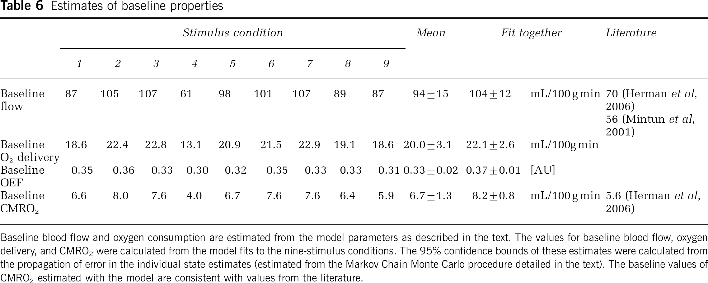
Baseline blood flow and oxygen consumption are estimated from the model parameters as described in the text. The values for baseline blood flow, oxygen delivery, and CMRO₂ were calculated from the model fits to the nine-stimulus conditions. The 95% confidence bounds of these estimates were calculated from the propagation of error in the individual state estimates (estimated from the Markov Chain Monte Carlo procedure detailed in the text). The baseline values of CMRO₂ estimated with the model are consistent with values from the literature.

Flow—Volume and Flow—Consumption Ratios

From the functional responses, we found that the ratio of maximum flow to maximum volume changes was 2.84 (range 2.83 to 2.85). There was a small increasing trend in this ratio with stimulus condition (R² = 0.78; P < 0.006 one-way ANOVA). This value was consistent with existing literature values of 2.33 (hypercapnic challenge) (Wu et al, 2002) but lower than those reported in functional studies 5 to 6 (sensory stimulation) (Mandeville et al, 1999a). Note that attention must be given to the vascular compartments averaged in estimating the flow—volume ratio as inclusion of the arterial compartment will produce smaller estimates of the ratio then when considering only the capillary and venous compartments.

We also found that the ratio of maximum CMRO₂ change to maximum flow change was 0.40 ± 0.05. This also did not vary significantly with stimulus condition (one-way ANOVA). The estimates of these values were more conserved in the joint fitting results. Previous studies in humans have reported values of the CMRO₂:flow ratio of 0.56 ± 0.8 (Hoge et al, 2005) and 0.3 (Kastrup et al, 2002), which are consistent with our reported values here.

Compartmentalized Changes in Hemodynamics

In Figure 8, we show the predicted hemodynamic changes in each of the vascular compartments for stimulus condition 9. The time courses of blood flow and oxy-, deoxy-, and total-hemoglobin changes are shown for the three vascular compartments and the modeled observation (i.e., the sum or mean of the three compartment changes shown in equation (15)). The neighboring plots show the time course of the initial response from 0 to 2 (3) seconds after stimulus. We found similar dynamic behavior with the model fits to the other eight experimental conditions. We did not note any differences between the independent and the joint estimates for the nine conditions.

Figure 8

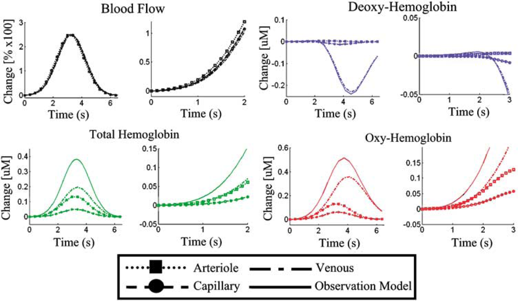
Compartmental hemodynamic changes: Vascular changes were modeled in the arterial, capillary, and venous compartments. The time courses plotted here from the ninth stimulus condition show the representative changes in these three compartments. The solid lines show the predicted observation model for either laser speckle imaging (blood flow) or spectroscopic imaging. The figures to the right of each plot show an enlargement of the initial onset regions.

Discussion

We have showed that the model proposed in this work was able to reproduce the majority of the measured hemodynamic responses, as noted by the large R² values for the model fits to each condition shown in Table 5.

In the model fits to the parametric whisker stimulus, our estimates of the change in CMRO₂ and arterial dilation increased linearly with stimulus amplitude (R² = 0.87 and 0.96, respectively). We were able to estimate these changes independently for the nine conditions and jointly by estimating these changes using the complete parametric data and assuming common values for baseline properties for the nine conditions. We found that the parameter estimates were consistent whereas the variance decreased for the joint estimation as expected.

We used Monte Carlo methods to verify that the state estimates were robust to the starting position of the minimization routine. We also verified that the model estimated consistent values for all nine stimuli conditions for the state variables representing structural and baseline properties as hypothesized. This finding supports the utility of the model to infer details of the vascular anatomy.

Multi- Versus Single-Compartment Models

We found that the higher temporal resolution and spectroscopic information of optical imaging requires a more detailed model than previously shown single-compartment models (Buxton et al, 1998, 2004; Mandeville et al, 1999b), In agreement with previous work (Zheng et al, 2005), we found that the multicompartment model performed better than the single-compartment formulation, even after the additional degrees-of-freedom for the more complicated model were accounted for (P < 8 × 10⁻⁵). Both models accurately reproduced the relationship between flow and volume, as indicated by the goodness-of-fit of blood flow and volume measurements by both models (refer Table 5), consistent with the previous report by Zheng et al (2005). Although estimates of arterial dilation were significantly higher in the single-compartment model (P < 2 × 10⁻⁶), both models predicted a linear relationship with stimulus condition (R² = 0.98 (single) and R² = 0.96 (multi)).

Further, we found that the multicompartment model performed significantly better at modeling oxy- and deoxy-hemoglobin measurements and the overall data set. The single-compartment model had significantly lower R² values for model fits to oxy- and deoxy-hemoglobin data in all nine stimulus conditions than the multicompartment model. We found that the CMRO₂ changes predicted by the multicompartment model were significantly better correlated with stimulus condition than the single-compartment model (R² = 0.08 (single) and R² = 0.87 (multi)). Owing to the large variance in the estimate of CMRO₂ changes in the single-compartment model, the difference in the two estimates was not statistically different (paired T-test).

Compartmentalized Changes in Hemodynamics

The predicted response curves for each of the vascular compartments, shown in Figure 7, are in qualitative agreement with previously published experimental findings (Vanzetta et al, 2005). We found that the largest magnitude of blood volume changes originated from the venous compartment whereas the arterial compartment had the largest fractional volume changes. Blood volume changes in the arteries initiated and peaked slightly before the volume changes in the capillaries and veins.

We found that the magnitude of the change in blood flow response of all three compartments was nearly identical but slightly lagged from the arterial to venous compartments consistent with Zheng et al (2005). In addition, we found that the majority of the contrast of oxy- and deoxy-hemoglobin changes arose from the venous structures. These large changes are the result of the large washout effects in this compartment with the lowest initial SO₂. We estimated venous oxygen saturation to be around 62% to 66%, which allows large changes in the blood oxygenation in response to the same magnitude of increased blood flow and volume changes as the other compartments. In comparison, the oxygen saturation of the arterial (95%) is very close to that of the feeding artery (98.7%) and changes in oxy- and deoxy-hemoglobin arise from blood volume changes with little influence of flow. We also observed larger and more latent oxyhemoglobin changes then total-hemoglobin that can be explained by the contribution of blood flow changes, which wash out the baseline deoxy-hemoglobin concentration.

Total oxygen content in tissue depends on contributions from arteries, veins, and capillaries. We find that at baseline the arteries and veins supplied 34% (2.8 ml O₂/100 g min) of the total oxygen delivered to the tissue (13% arterial; 21% venous) with the capillary compartment supplying the remaining 66% (5.4 ml O₂/100 g min). Comparable theoretical modeling predicts that 70% of oxygen exchange to tissue occurs through the capillaries (Sharan and Popel, 2002).

Another important contribution made in this model is allowance for dynamic changes in tissue oxygenation. In qualitative agreement with recent work examining stimulus-evoked tissue oxygenation (Offenhauser et al, 2005), we found that tissue oxygenation (p_tissueO₂) changes were biphasic. During early onset of the response (1 to 2 secs), an initial dip (i.e., -8% for condition 9) in the tissue oxygenation was observed coinciding with an increase in CMRO₂. After the return of CMRO₂ to baseline, the tissue oxygenation was observed to surpass its baseline value (i.e., +28% for condition 9).

Determination of Baseline Properties

A key feature of our model is the bottom-up methodology that allows us to recover baseline blood volume and oxygenation properties of the tissue from the measured hemodynamic responses. The estimates of the baseline oxygen delivery (20.0 mL O₂/100 g min) and CMRO₂ (6.7 mL O₂/100 g min) calculated with this model are consistent with the physiologic ranges reported in the previous literature (Habler and Messmer, 1997; Mintun et al, 2001; Herman et al, 2006). Our estimates of blood flow are slightly higher than those found in the literature. This could be explained by the assumption for the hemoglobin content of blood, which affects the absolute magnitude of the blood flow response. Baseline OEF was also calculated based on using the values of baseline oxygen saturation and was found to be 0.37 ± 0.01, which is within the range in previously published results that have suggested a wide range of values (0.2 to 0.7) (Buxton et al, 2004; Zheng et al, 2002, 2005).

Model Assumptions and Future Extensions

There are several assumptions and model simplifications presented in this work, which are important to recognize in the context of interpreting these results. Concerning the estimation of absolute functional and baseline parameters, this calculation relies on the quantitative accuracy of both measurement methods. In this work, we have assumed that optical spectroscopy can provide a measure of absolute hemoglobin changes. This accuracy depends on the propagation of light in the tissue and the path length correction applied to calculate hemoglobin changes from the optical spectroscopy. The absolute quantities of blood flow, volume, and CMRO₂ are calculated by scaling between the model and the measurements using relative amplitudes and time courses of each predicted hemodynamic change and the actual magnitudes of the experimental data. Thus, uncertainties in the model estimates are linear with uncertainties in the absolute magnitude of the optical data, and thus dependent on systematic errors in the estimates of optical path length or partial volume errors in the measured data. However, the estimate of relative changes in CMRO₂, blood flow or volume are unaffected by these errors. These errors will limit the estimation of absolute, but not relative, changes in noninvasive human imaging with methods such as fMRI or diffuse optical imaging. In this work, we assumed laser speckle to provide a relative measure of blood flow changes as showed by comparison with laser Doppler (Dunn et al, 2001). However, the speckle imaging techniques make assumptions about the relationship between velocity and flow, which need to be considered in more detail in the future.

Conclusions

We conclude that the proposed multiple compartment model makes the following significant contributions: (i) The multicompartment model shows significant improvements in the modeling of measured oxy- and deoxy-hemoglobin changes. (ii) The bottom-up framework of this model allows for inclusion of multimodality data in a Bayesian model. This setup improves the accuracy of the estimated states by compensating for uneven measurement noise across modalities and can be readily extended to the analysis of human functional neuroimaging measurements. (iii) Our model allows the estimation of baseline hemodynamic and metabolic parameters from the time courses of dynamic hemodynamic measurements. We can use the relationship between absolute and relative changes in hemoglobin concentration to estimate baseline blood volume and oxygen consumption. This feature offers a significant improvement over previous models and could open the door to examine differences in baseline hemodynamic properties in normal and disease models.

Footnotes

Acknowledgements

TJH is funded by the Howard Hughes Medical Institute predoctorial fellowship program. MSA is funded by the Rudolph Hermann Doctoral fellowship at UTA.

References

Aguirre

Zarahn

D'Esposito

(1998) The variability of human, BOLD hemodynamic responses. Neuroimage 8:360–9

Berwick

Redgrave

Jones

Hewson-Stoate

Martindale

Johnston

Mayhew

(2004) Integration of neural responses originating from different regions of the cortical somatosensory map. Brain Res 1030:284–93

Boas

Strangman

Culver

Hoge

Jasdzewski

Poldrack

Rosen

Mandeville

(2003) Can the cerebral metabolic rate of oxygen be estimated with near-infrared spectroscopy? Phys Med Biol 48:2405–18

Briers

(2001) Laser Doppler, speckle and related techniques for blood perfusion mapping and imaging. Physiol Meas 22:R35–66

Buxton

Frank

(1997) A model for the coupling between cerebral blood flow and oxygen metabolism during neural stimulation. J Cereb Blood Flow Metab 17:64–72

Buxton

Uludag

Dubowitz

Liu

(2004) Modeling the hemodynamic response to brain activation. Neuroimage 23(Suppl 1):S220–33

Buxton

Wong

Frank

(1998) Dynamics of blood flow and oxygenation changes during brain activation: the balloon model. Magn Reson Med 39:855–64

Carter

Kohn

(1996) Markov Chain Monte Carlo in Conditionally Gaussian State Space Models. Biometrika 83:589–601

Devor

Dunn

Andermann

Ulbert

Boas

Dale

(2003) Coupling of total hemoglobin concentration, oxygenation, and neural activity in rat somatosensory cortex. Neuron 39:353–9

10.

Devor

Ulbert

Dunn

Narayanan

Jones

Andermann

Boas

Dale

(2005) Coupling of the cortical hemodynamic response to cortical and thalamic neuronal activity. Proc Natl Acad Sci USA 102:3822–7

11.

Devore

(1995) Simple linear regression and correlation probability and statistics for engineering and the sciences. Belmont, CA, USA: Wadsworth Inc, 474–522

12.

Dunn

Bolay

Moskowitz

Boas

(2001) Dynamic imaging of cerebral blood flow using laser speckle. J Cereb Blood Flow Metab 21:195–201

13.

Dunn

Devor

Dale

Boas

(2005) Spatial extent of oxygen metabolism and hemodynamic changes during functional activation of the rat somatosensory cortex. Neuroimage 27:279–90

14.

Duong

Kim

(2000) In vivo MR measurements of regional arterial and venous blood volume fractions in intact rat brain. Magn Reson Med 43:393–402

15.

Girouard

Iadecola

(2006) Neurovascular coupling in the normal brain and in hypertension, stroke, and Alzheimer disease. J Appl Physiol 100:328–35

16.

Habler

Messmer

(1997) The physiology of oxygen transport. Transfus Sci 18:425–35

17.

Herman

Trubel

Hyder

(2006) A multiparametric assessment of oxygen efflux from the brain. J Cereb Blood Flow Metab 26:79–91

18.

Hoge

Franceschini

Covolan

Huppert

Mandeville

Boas

(2005) Simultaneous recording of task-induced changes in blood oxygenation, volume, and flow using diffuse optical imaging and arterial spin-labeling MRI. Neuroimage 25:701–7

19.

Kastrup

Kruger

Neumann-Haefelin

Glover

Moseley

(2002) Changes of cerebral blood flow, oxygenation, and oxidative metabolism during graded motor activation. Neuroimage 15:74–82

20.

Kocsis

Herman

Eke

(2006) Mathematical model for the estimation of hemodynamic and oxygenation variables by tissue spectroscopy. J Theor Biol 241:262–75

21.

Kohl

Lindauer

Royl

Kuhl

Gold

Villringer

Dirnagl

(2000) Physical model for the spectroscopic analysis of cortical intrinsic optical signals. Phys Med Biol 45:3749–64

22.

Mandeville

Marota

Ayata

Moskowitz

Weisskoff

Rosen

(1999a) MRI measurement of the temporal evolution of relative CMRO(2) during rat forepaw stimulation. Magn Reson Med 42:944–51

23.

Mandeville

Marota

Ayata

Zaharchuk

Moskowitz

Rosen

Weisskoff

(1999b) Evidence of a cerebrovascular postarteriole Windkessel with delayed compliance. J Cereb Blood Flow Metab 19:679–89

24.

Marquardt

(1963) An algorithm for least-squares estimation of nonlinear parameters. J Soc Indust Appl Math 11:431–41

25.

Mintun

Lundstrom

Snyder

Vlassenko

Shulman

Raichle

(2001) Blood flow and oxygen delivery to human brain during functional activity: theoretical modeling and experimental data. Proc Natl Acad Sci USA 98:6859–64

26.

Nair

(2005) About being BOLD. Brain Res Brain Res Rev 50:229–43

27.

Nielsen

Fabricius

Lauritzen

(2000) Scanning laser-Doppler flowmetry of rat cerebral circulation during cortical spreading depression. J Vasc Res 37:513–22

28.

Offenhauser

Thomsen

Caesar

Lauritzen

(2005) Activity-induced tissue oxygenation changes in rat cerebellar cortex: interplay of postsynaptic activation and blood flow. J Physiol 565:279–94

29.

Riera

Aubert

Iwata

Kawashima

Wan

Ozaki

(2005) Fusing EEG and fMRI based on a bottom-up model: inferring activation and effective connectivity in neural masses. Philos Trans R Soc London B Biol Sci 360:1025–41

30.

Severinghaus

(1979) Simple, accurate equations for human blood O₂ dissociation computations. J Appl Physiol 46:599–602

31.

Sharan

Popel

(2002) A compartmental model for oxygen transport in brain microcirculation in the presence of blood substitutes. J Theor Biol 216:479–500

32.

Sheth

Nemoto

Guiou

Walker

Toga

(2005) Spatiotemporal evolution of functional hemodynamic changes and their relationship to neuronal activity. J Cereb Blood Flow Metab 25:830–41

33.

Tsai

Johnson

Intaglietta

(2003) Oxygen gradients in the microcirculation. Physiol Rev 83:933–963

34.

Vanzetta

Hildesheim

Grinvald

(2005) Compartment-resolved imaging of activity-dependent dynamics of cortical blood volume and oximetry. J Neurosci 25:2233–44

35.

Vovenko

(1999) Distribution of oxygen tension on the surface of arterioles, capillaries and venules of brain cortex and in tissue in normoxia: an experimental study on rats. Pflugers Arch 437:617–23

36.

Washburn

(1921) The Dynamics of Capillary Flow. Physics Review Letters 12:273–83

37.

Watanabe

Harada

Kosaka

Shiga

(1994) Intravital microreflectometry of individual pial vessels and capillary region of rat. J Cereb Blood Flow Metab 14:75–84

38.

Luo

Zhao

(2002) Transient relationships among BOLD, CBV, and CBF changes in rat brain as detected by functional MRI. Magn Reson Med 48:987–93

39.

Zheng

Johnston

Berwick

Chen

Billings

Mayhew

(2005) A three-compartment model of the hemodynamic response and oxygen delivery to brain. Neuroimage 28:925–39

40.

Zheng

Martindale

Johnston

Jones

Berwick

Mayhew

(2002) A model of the hemodynamic response and oxygen delivery to brain. Neuroimage 16:617–37

A Multicompartment Vascular Model for Inferring Baseline and Functional Changes in Cerebral Oxygen Metabolism and Arterial Dilation

Abstract

Keywords

Introduction

Theory

General Description of Multi-Compartment Model

Vascular Model

Arterial Dilation

Oxygen Transport Model

CMRO2

Measurement Models

Materials and methods

Experimental Methods

Results

Multicompartment Estimates

Joint Estimates Using all Stimulus Conditions

Model Uniqueness

Comparison to the Single-Compartment Windkessel Model

Estimated Baseline Properties

Flow—Volume and Flow—Consumption Ratios

Compartmentalized Changes in Hemodynamics

Discussion

Multi- Versus Single-Compartment Models

Compartmentalized Changes in Hemodynamics

Determination of Baseline Properties

Model Assumptions and Future Extensions

Conclusions

Footnotes

Acknowledgements

References