
Abstract
This article deals with the problem of model selection for the mathematical description of tracer kinetics in nuclear medicine. It stems from the consideration of some specific data sets where different models have similar performances. In these situations, it is shown that considerate averaging of a parameter's estimates over the entire model set is better than obtaining the estimates from one model only. Furthermore, it is also shown that the procedure of averaging over a small number of “good” models reduces the “generalization error,” the error introduced when the model selected over a particular data set is applied to different conditions, such as subject populations with altered physiologic parameters, modified acquisition protocols, and different signal-to-noise ratios. The method of averaging over the entire model set uses Akaike coefficients as measures of an individual model's likelihood. To facilitate the understanding of these statistical tools, the authors provide an introduction to model selection criteria and a short technical treatment of Akaike's information–theoretic approach. The new method is illustrated and epitomized by a case example on the modeling of [11C]flumazenil kinetics in the brain, containing both real and simulated data.
Keywords
Hirotugu Akaike introduced the Akaike information coefficient (AIC) in 1973 (Akaike, 1973). Since then, the AIC has become a standard tool for model selection in regression analysis.
One interesting and usually overlooked feature of AIC is that the coefficient is an estimator of the Kullback-Leibler (K-L) distances of the models from the true generating mechanism of the data (Kullback and Leibler, 1951), regardless of whether the true model is in the set. This property is indeed quite powerful and has important consequences. First, it neatly formalizes the vague notion that no “true” model for the data exists. Truly the very word model implies simplification and idealization. Modeling has been defined as the process of constructing idealized representations that capture important aspects of complex biologic and physical systems (Chatfield, 1995). Second, if the “true” model does not exist, then the notion of a model selection procedure that selects the “best” model and discards others may lose appeal. An alternative possibility is that there may be more than one model that can be regarded as useful (i.e., able to provide a sufficiently close approximation to the data for the purpose at hand) (Chatfield, 1995). Third, recent work in statistics has shown that procedures that select the best model from a set, particularly in regression analysis, are intrinsically unstable (Breiman, 1996). This means that the model selection procedure introduces an amount of variance comparable to the error due to parameter estimation. Regression procedures can be “stabilized,” however, by appropriate averaging of parameter values over the entire model set (Breiman, 1996).
These considerations can be developed, with minimal conceptual and technical effort, into a new paradigm of “model weighted averaging” where estimates of the parameter of interest are obtained from the entire model class or a suitable subset (Buckland et al., 1997). This article introduces a model averaging approach into the context of classical compartmental modeling. Its evaluation will be carried out using illustrative data generated with positron emission tomography (PET).
THEORETICAL BACKGROUND
The problem of estimating the dimension of a model occurs in various forms in applied statistics (e.g., multiple linear and nonlinear regression, factor analysis, time-series modeling). Most of the foundations of the subject were laid down in the mid 1970s. The Cp criterion of Mallows (1973) and the PRESS criterion of Allen (1974) were introduced for use with linear regression. At the same time more widely applicable approaches were developed, including AIC, the cross-validation method (Stone, 1974), the Bayesian information coefficient (BIC) (Schwarz, 1978), and minimum description length (Rissanen, 1978). Work has proceeded on the lines of these methods and modified as well as new criteria have appeared in the literature (Burnham and Anderson, 1998).
Buckland et al. (1997) advocated the approach of model averaging introduced here, but the approach had been considered in the original work of Akaike (1978b, 1979). The model averaging approach is based on AIC by reasons of its information-theoretic background, its formal links to maximum likelihood (ML) theory, and its fundamental connections to the area of the foundations of statistics. These aspects will be briefly reviewed in the following sections. Since a model-averaging paradigm exists in the Bayesian framework, the relation between AIC, BIC, and Bayesian inference will be also sketched for the sake of completeness and clarity.
The Kullback-Leibler distance
The K-L distance between the models f and g is defined as:
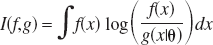
The function f is considered fixed, whereas g varies over a space of models indexed by its parameter vector θ. X is the sample space where x ε X. I(f,g) is amenable to two interpretations. One is of “information loss” when g is used to approximate f, and the second is of “distance” of g from the data-generating process f.
I(f,g) is a fundamental measure of information and is related to other information quantifiers (Soofi, 1994). If f is defined on the same parameter space of g (i.e., f(x) = g(x|θ0)), then for θ → θ0 I(f,g) is equal to the Fisher information matrix (Kullback and Leibler, 1951). I(f,g) has relations to the general concept of entropy H(x) = –log(f(x)) originated by Boltzmann (1877), to Shannon's entropy H(x) = ∫f(x) log (f(x)) dx in communication theory (Shannon, 1948) and can be interpreted as the cross-entropy between f and g (Soofi, 1994).
Estimation of Kullback-Leibler information
Akaike (1973) developed an estimator of the expected K-L information based on the maximized log-likelihood function. This finding makes it possible to combine ML estimation and model selection in a unified optimization framework. The criterion has a large sample formulation as:
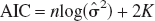
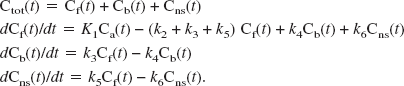
where log(L( ) is the value of the maximized log-likelihood over the unknown parameter vector θ, given the data and the model. K is the number of estimable parameters in the model. In the special case of least-squares estimation with normally distributed errors, apart from an additive constant, AIC can be expressed as:

with

where  are the estimated residuals from the fitted model and n is the sample size. In this case the number of estimable parameters is equal to the number of model parameters plus 1 for
  . In case of unequal variance at different time points, model estimates can be obtained by weighted least squares and the formula can be extended using the weighted residuals in place of
  . Note that the additive constant depends on the number of samples, n, but not on the number of parameters, K, thereby allowing comparisons among models only for a given data set.
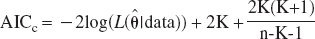
Assuming a set of M candidate models, AIC is computed for each model and the one with minimal AIC is selected. The selected model is also the one with minimal K-L distance from the true (unknown) data generating mechanism f. When K is large relative to n (n/K ≲ 40), the small sample formulation (Hurvich and Tsai, 1989; Sugiura, 1978) should be used as:
Model likelihood and Akaike weights
Define now:
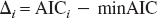
where minAIC is the minimum value of AIC for the model set. The likelihood of each model gi conditional to the data and to the model set is (Akaike, 1983):
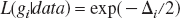
Therefore, one can compare models within a set by looking at their likelihood ratios. Note that an alternative interpretation of AIC is of a maximized-likelihood estimate where the right-hand term of Eq. 2a is a bias-correction factor due to the fact that both  and
and  are calculated from the same data set.
Since all L(gi|data) are conditional on the set of M models, it is appropriate to introduce the normalized coefficients:
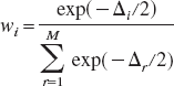
The coefficients wi, or “Akaike weights” (Burnham and Anderson, 1998), can therefore be interpreted as “weight of evidence” in favor of model i within the set (Akaike, 1978a, 1979, 1980, 1981; Buckland et al., 1997).
Akaike weights, model uncertainty, and model generalization
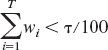
The Akaike weights possess an interesting interpretation in the model uncertainty framework. Suppose that each of the M models is a discrete point in a model space

represents the τ% confidence set conditional to the data and
This concept may be useful in the context of model selection and generalization (Breiman, 1996). In nuclear medicine, generalization refers to the common practice of selecting a model for a particular tracer on an initial data set (which we can refer to as the calibration set) and then applying this model for all subsequent studies.
The problem is that the calibration set may differ in terms of sampling, noise conditions, and parameter space from subsequent sets. For example, scan duration or time sampling may vary among studies due to technical or clinical constraints. Noise levels may also vary because of the amount of injected radioactivity, scanner type, as well as the size of the ROI. In addition, the calibration group may not be representative of a pathological population, nor indeed of the normal population (e.g., because of gender or age differences).
Therefore, unless the τ% confidence set (say, 90% confidence set) contains one model only, it may be appropriate not to discard the other models because these could provide better performance on slightly different sampling spaces.
Model averaging using Akaike weights
The concept developed in the Introduction considered a small model set where each model is a useful approximation of the data-generating process. By useful it is meant that from each model one can obtain estimations of θi sufficiently close to the true value of the parameter of interest, θ. The relative “closeness to the truth” of each model can be quantified in the K-L metric with AIC.
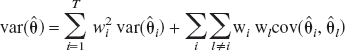
Therefore, instead of obtaining estimates of θ from the best model in the set, one can use the Akaike weights to calculate:
where  is the ML estimate of θ in model i (Buckland et al., 1997). Obviously, θ is assumed to be common to all models.
Note that T in Eq. 6 can be determined in two very different ways. First, one can set T = M and therefore use all the models in the set. This is appropriate if M is small and the set has been defined on previous experiments. If the set is too big, however, or if some models give little or no contribution to the final estimate (i.e., their Akaike weights are generally small), then it may be appropriate to restrict the model set by setting a threshold τ as explained previously. In this case an additive uncertainty will be added owing to the model class selection procedure, but we may expect that this contribution to the total variance will be smaller than using models that have little to do with the data.
Estimates for var( ) can be obtained from linear combinations of var(
 ) plus a component representing model misspecification bias.
Following Buckland's formalization (Buckland et al., 1997), let βi = θ – θi be the bias arising in estimating θ under model i. Suppose further that E(βi) = 0 where expectation is taken over all possible models. Define:
Taking expectation over all possible models of this expression gives  .
.
Denote now: 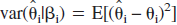 and
and 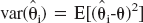 , then
 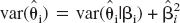 . This yields:

where the covariance term accounts for all models being estimated on the same data set. The covariance term will be in general unknown; however one can take, as an estimate, its upper bound that is equal to the geometric mean of var(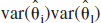 )var(
)var( ) (Buckland et al., 1997). This gives:
Variance in Eq. 8 can be estimated by substituting  and
and  . Alternatively, var(
 ) can be obtained from Eq. 7 using bootstrap resampling (Buckland et al., 1997). See Efron and Tibshirani (1993) for an introduction to the bootstrap and Turkheimer et al. (1998) for an application of bootstrap to PET data.
Relation to other model-selection criteria
The framework developed so far does not fit the AIC criterion uniquely. Consider for example the BIC criterion (Schwarz, 1978). By defining Δi = BICi – minBIC analogously to Eq. 3, then exp(–Δi/2) is equal to the posterior probability of model i conditional on model space
Applications to compartmental modeling
Although the theory developed so far is of general use, this article focuses on the class of compartmental models used in PET for the kinetic modeling of TACs (Gunn et al., 2001; Mazoyer et al., 1986). In this context, AIC has been extensively used for model selection, and Hawkins et al. (1986) is usually the original reference for its application to PET.
The general setup for the model selection problem in PET may assume that a set M is defined consisting of a small number of physiologically meaningful compartmental models. No recipe for the definition of M is provided here. Indeed, this is not a statistical problem; model construction is a fundamental activity that is based on the existing knowledge about the system of interest (Chatfield, 1995).
In general terms, it is expected that M will contain a small number of models with a certain number of compartments. Models may not be necessarily nested, and some of models' parameters may be fixed. M may contain simultaneously models calculated over different input functions (e.g., sampled from blood, a reference region, or any other type of tomographic measurement).
Note that this framework does not apply to graphical methods like the Patlak (Gjedde, 1981; Patlak and Blasberg, 1985) or the Logan plot (Logan et al., 1990) because they are applied to reduced sets of data, the estimations are independent of the number of compartments, and, in the case of the Logan plot, they do not provide estimates in the ML sense.
Therefore, the ensuing section will evaluate the usefulness of Akaike weights in the model selection problem over such model class.
EXPERIMENTAL SECTION
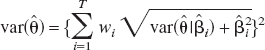
The problem of model selection is common to all tracers used in PET. For the sake of clarity, this section focuses on the kinetic analysis of those radioligand studies that enable the quantitative description of neuroreceptor binding sites in the brain (Cunningham and Lammerstma, 1994; Mintun et al., 1984). A general analysis of compartmental models in PET is presented by Gunn et al. (2001), where a distinction is made between “macro” parameters (e.g., the total volume of distribution), which have the same interpretation across a set of particular compartmental models, and “micro” parameters, the interpretation of which is model specific. In this context, we consider the general compartmental model illustrated diagrammatically in Fig. 1A. This model represents the possible exchanges of the tracer between a vascular (plasma) compartment and three tissue compartments: a “free” pool, a “non–specifically bound” pool, and a “specifically bound” pool. The corresponding rate equations for this model are as follows:

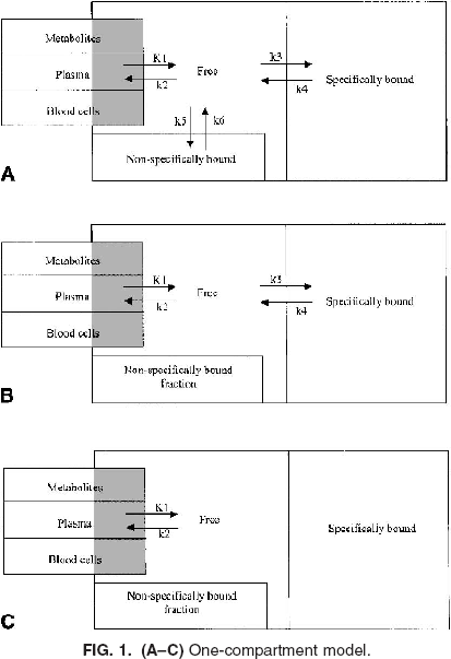
Ctot(t) denotes the total concentration of radioligand in the tissue as a function of time, comprising free (Cf(t)), non–specifically bound (Cns(t)), and specifically bound (Cb(t)). It is here assumed that measures of the concentration of label in arterial whole blood [Cwb(t)] and of the parent radioligand in arterial plasma [input function Ca(t)] are available. It is also assumed that radiolabeled metabolites of the parent in plasma do not cross the blood–brain barrier.
K1 and k2 – k6 are the rate constants; K1 is the unidirectional clearance of the ligand from plasma to tissue whereas k2 models the clearance from tissue to plasma; k5 and k6 model the exchanges of the free tissue compartment with the nonspecific binding space; k3 = Kon Bavail, where Kon is the bimolecular association rate constant and Bavail is the concentration of available binding sites; and k4 = Koff is the dissociation rate constant of the ligand-binding site complex. Finally, because of the limited spatial resolution of PET, the total PET signal comprises also label in the vasculature. Denoting the vascular volume fraction as Vb yields:
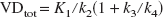
The parameter of interest in this model is usually the ratio k3/k4 termed “binding potential” (Mintun et al., 1984). A simplification often used is the description of the radioligand uptake in terms of volume of distribution. The total volume of distribution (VDtot) is the partition ratio between the total concentration of ligand in the tissue and that in plasma that would be attained in a steady-state equilibrium between the two. The estimate of this parameter is generally more stable than the estimates of microparameters (K1, k2- k6) and can be calculated as:
The three compartments model can be simplified to two compartments (Fig. 1B) by assuming a fast equilibration between the free and the nonspecific fractions in the tissue (Koeppe et al., 1991). In this case, the volume of distribution is calculated as:
If tissue compartments are indistinguishable than the model reduces to one compartment only (Fig. 1C). Concurrently VDtot becomes:
The compartment model above is here defined for illustrative purposes only. There is no suggestion that this model is generally “right” or that it is the most practical.
Measured data set: Modeling ligand binding to the GABA receptor
For several radioligands, the difference in fit quality between models is small (Carson et al., 1998; Lammertsma et al., 1996). As an example, this section focuses on the kinetic modeling of ligands binding to the central benzodiazepine (GABA) receptor in the brain. Consider the data of Koeppe et al. (1991) on the compartmental modeling of [11C]flumazenil, a high-affinity antagonist for GABA receptors.
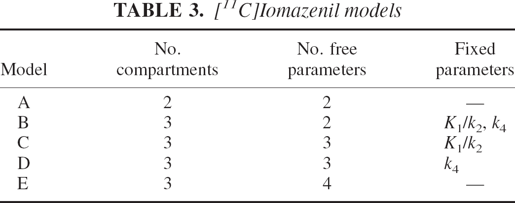
In this study, three models were considered. The first, the two-parameter model, is shown in Fig. 1C. The second, the three-parameter model, is the two-compartment model shown in Fig. 1B where the ratio K1/k2 was fixed to a value estimated with an ROI placed on the pons. The third is the four-parameter model shown in Fig. 1B with all parameters to be estimated. Blood volume, Vb, was inserted in all three models as estimated from the entire brain volume. For reasons that will be clearer later, we label these models respectively as model A, model C, and model E (Table 3).
For each model, the χ2 reported by Koeppe et al. (1991) for six ROIs averaged over six subjects were multiplied the degrees of freedom, e.g.,
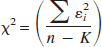
to obtain the sum of the squared residuals. The Akaike weights were then calculated as in Eq. 5 using the AICc of Eq. 2c and are shown in Table 1. Note that, since the χ2 were averaged, these weights are not mean weights, but weights relative to the mean likelihood.
Akaike information coefficient weights for [11C]flumazenil models
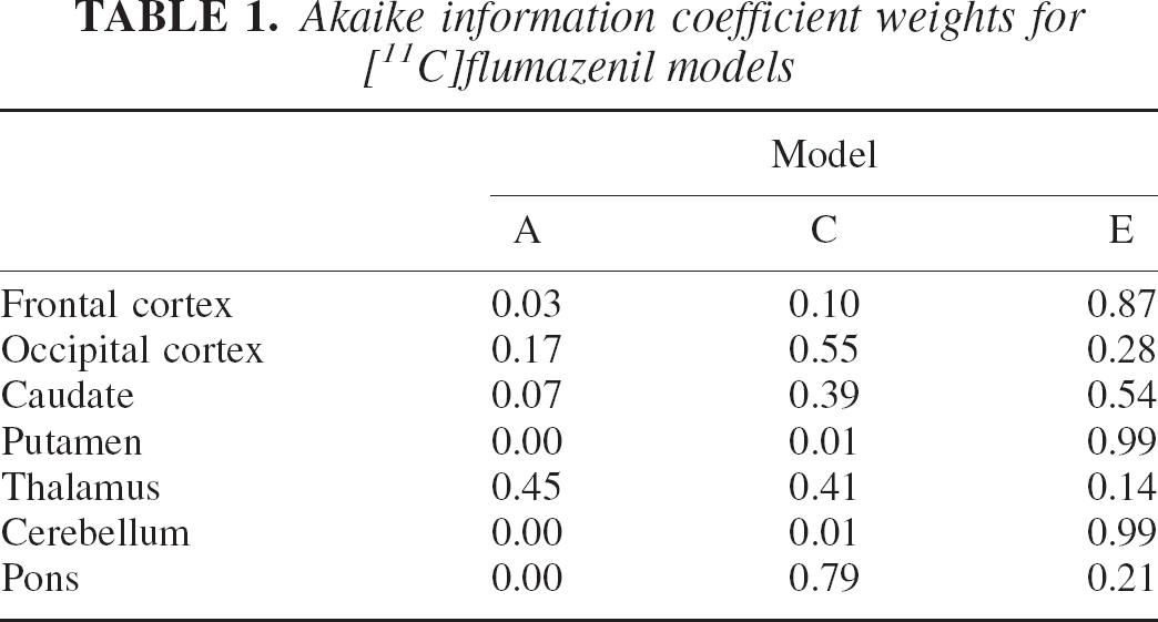
For the values of the estimated parameters the reader is referred to Table 2 where values are reported for use in a simulation study, or to the original reference. Analysis of Table 1 suggests that model E is selected with little uncertainty in half of the regions (frontal cortex, putamen, cerebellum). Selection is far less clear-cut in the other cases. In the thalamus, for example, all three models considered offer similar likelihoods.
Kinetic parameters for [11C]flumazenil simulation
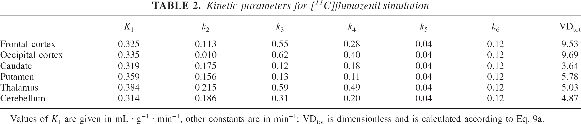
Values of K1 are given in mL · g–1 · min–1, other constants are in min–1; VDtot is dimensionless and is calculated according to Eq. 9a.
The data of Buck et al. (1996) provide further evidence that the problem relates more generally to the system being modeled and it is not peculiar of a single tracer or data set. In this case, the GABA receptor density was measured using [11C]iomazenil and a similar array of models was used. The data analysis considered the two-parameter model (model A following Buck's labeling), the four-parameter model (model E) and three subversions of it where either K1/k2 (model C) or k4 (model D) or both (model B) were fixed to preestimated values. These models are summarized in Table 3. The AICc values for Table 4 provides a picture very similar to the one provided by Table 1. In the case of the occipital cortex, the two-compartment model in its various arrangements (B, C, D, and E) provides similar likelihood. Note that although these models arise from the same compartmental structure, they provide numerical estimates of the parameters that differed markedly (Buck et al., 1996).
[11C]Iomazenil models
the five models are reported in Table 4 and were calculated for two regions (cerebellum and frontal cortex) and averaged over five subjects. The values were obtained from Table 2 of the original reference.
Akaike information coefficients weights for [11C]iomazenil models
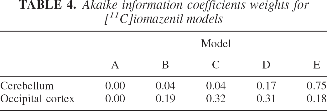
It is also remarkable that a region with low binding (i.e., the cerebellum) has consistently better fit with the maximum number of free parameters (model E). This observation echoes similar ones made in previous reports (Carson et al., 1998; Watabe et al., 2000) on the revealing fact that regions with little or no specific binding often require the most complex model. Most probably, the absence of a relatively large kinetic component due to specific uptake brings to the identifiability level a larger number of compartments, of comparable magnitude, that are involved in the nonspecific binding of the ligand. Alternatively, reference regions may be bigger than regions with specific binding and therefore possess a more favorable signal-to-noise ratio.
Synthetic data set: Simulated [11C]flumazenil study
The information acquired from the experimental data can now be used to attempt a numerical evaluation of the weighted average technique. The artificial data sets considered a “reality” similar to the one of the real data sets on [11C]flumazenil. Note that by “similar” it is not meant that we attempt to duplicate reality: this is not possible and, as it will be clear from the results, matching results between simulations and reality have not been obtained. Instead a scenario is created with useful similarities to these data.
The kinetic of [11C]flumazenil is simulated using the three-compartment, six-parameter model of Fig. 1A for six regions. Kinetic parameters for the regions were obtained from Koeppe et al. (1991) and are illustrated in Table 2. The constants for the nonspecific compartment (k5, k6) were obtained from k3, k4 values of the pons, where no specific binding is expected.
An artificial noiseless arterial input function resembling real ones was used to generate the TACs that consisted in 21 frames for a total of 60 minutes. Gaussian noise was then added to TACs with standard deviation proportional to the absolute activity in each frame. The noise proportionality constant varied from 5% for large regions (frontal and occipital cortex, cerebellum) to 7% or 8% for the smaller ones (caudate, putamen, thalamus) to match real conditions.
The simulation considered the estimation of the same three models used by Koeppe et al. (1991) and described in the previous section. Note that none of these models considers the additional third compartment simulating nonspecific binding of the tracer. This was arranged with the purpose of having the supposedly “true” model outside the model set. Indeed this situation may be quite realistic given that many tracers bind to nonspecific sites and PET data do not usually allow the estimation of models with more than three compartments.
Model parameters were estimated using a nonlinear least-square procedure performed using the Nelder-Mead simplex minimization routine (Nelder and Mead, 1965). Software was written in Matlab (The Mathworks Inc., MA, U.S.A.) and run on an Ultra-Sparc 10 Sun Workstation (SunSystems, Mountain View, CA, U.S.A.). Volumes of distribution were calculated according to Eq. 9c (model A) and Eq. 9b (models C and E).
The first set of results contemplates an overall numerical comparison between the model averaging and model selection methods. Two hundred artificial data sets, each with six regional TACs, were generated and the three models estimated. For each TAC, AICc coefficients for the three models were calculated. The parameter of interest, in this case the total volume of distribution VDtot, was calculated either from the model with lowest AICc (model selection) or as a weighted average from the three models (as in Eq. 6) using the Akaike weights.
RESULTS
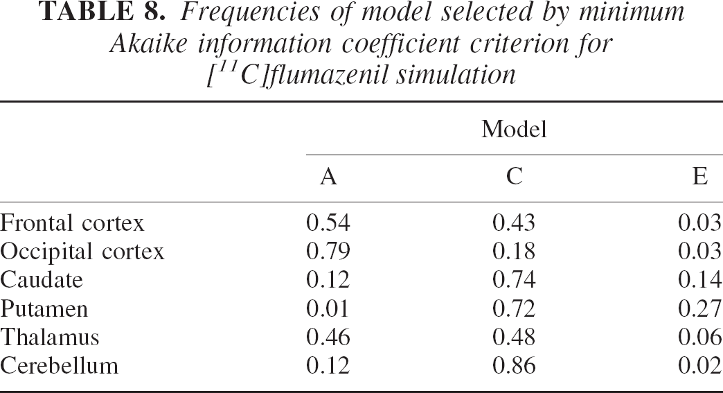
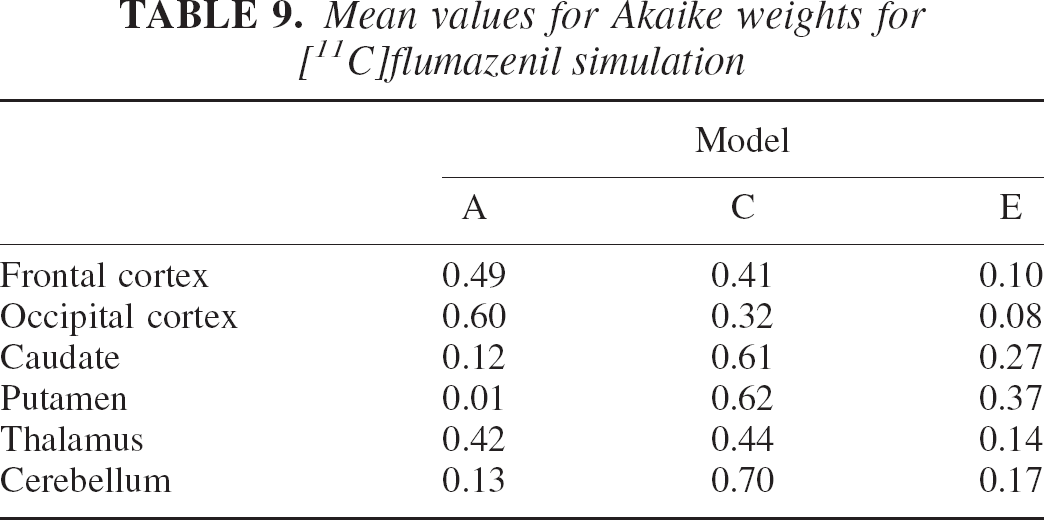
The results of the simulation are given in Tables 5, 6 and 7 in terms of percentage bias, standard deviation, and MSE over the estimated VDtot. Table 8 contains the frequencies of selection for each model by the minimum AICc procedure for the six regions. Table 9 shows the average weights for the AICc-weighted procedure.
Volume of distribution: bias for [11C]flumazenil simulation
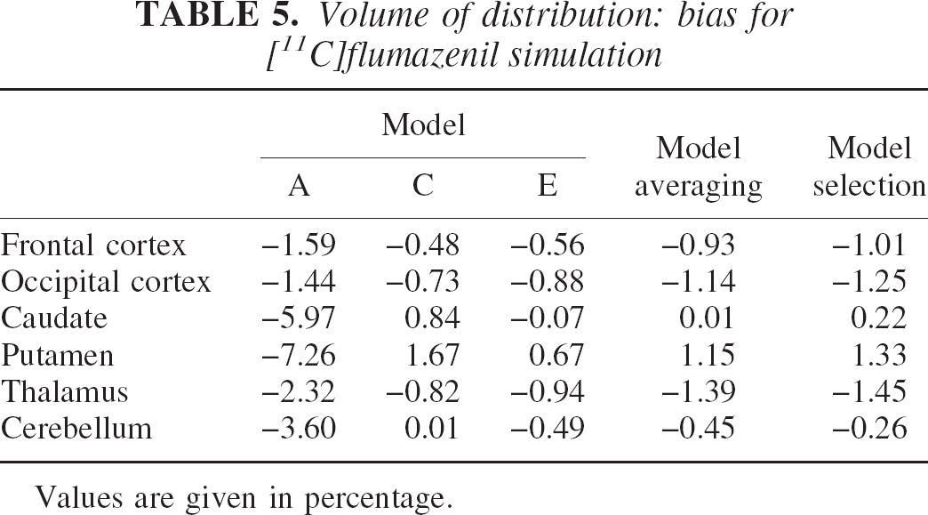
Values are given in percentage.
Volume of distribution: standard deviation for [11C]flumazenil simulation
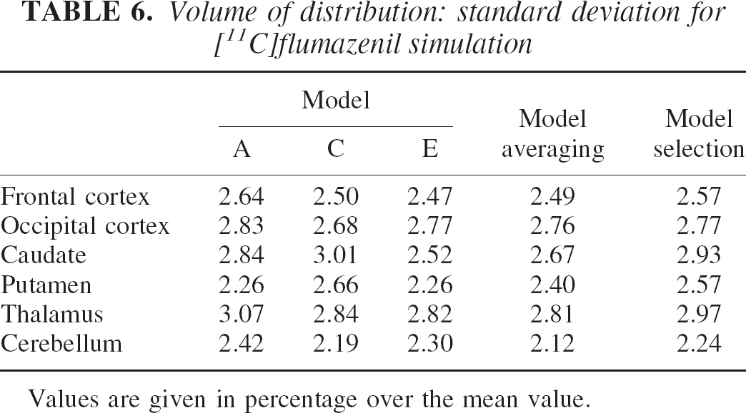
Values are given in percentage over the mean value.
Volume of distribution: mean squared error for [11C]flumazenil simulation
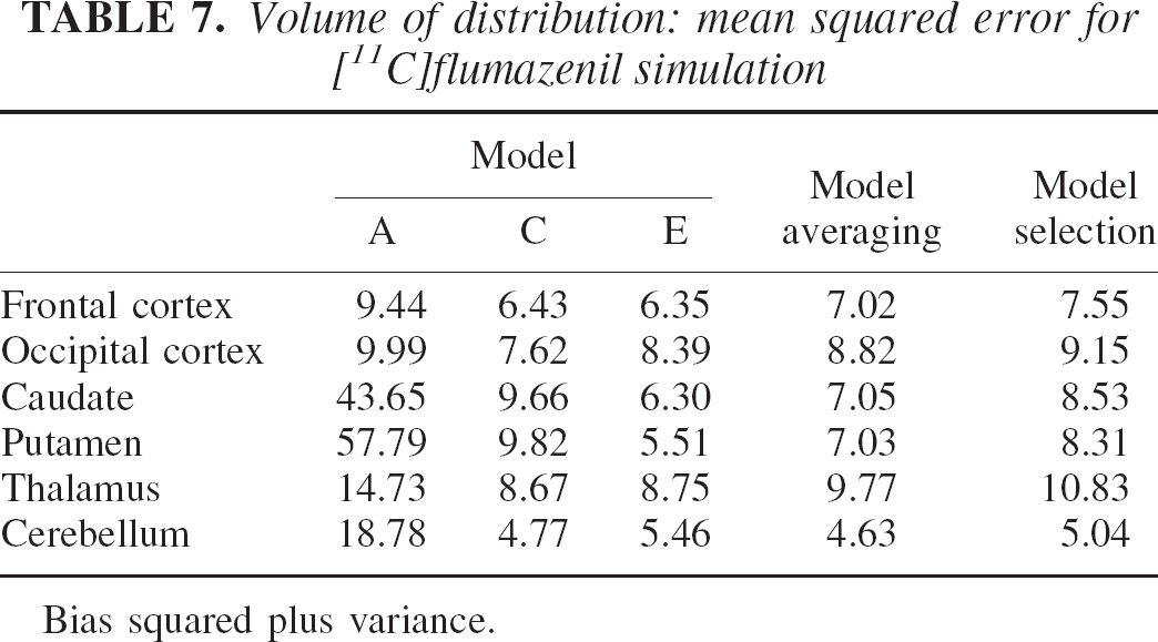
Bias squared plus variance.
Frequencies of model selected by minimum Akaike information coefficient criterion for [11C]flumazenil simulation
Mean values for Akaike weights for [11C]flumazenil simulation
Tables 5 and 6 and particularly the MSE values contained in Table 7 suggest that model E, the most complex model, performs better in the regions with lower specific uptake (i.e., the caudate and putamen), where the relative effect of the nonspecific component is greater. Instead, model C has slightly better results on the remaining regions. MSE values for model A are the highest for the three models in all regions and are reasonable only on the regions with high specific uptake (i.e., the cortex).
The model averaging method shows a general improvement of the MSE compared with that of the model selection that ranged from 21% to 10% in the low-uptake regions (caudate and putamen) and 8% to 4% in the remaining regions. Note in Table 9 how the AICc-weighted procedure balances all three models' contributions to obtain VDtot estimates.
Synthetic data set: Simulated [11C]flumazenil study revisited
The simulation results obtained so far can be used to deepen our analysis of the modeling process. Now consider that the previous comparison does not mimic exactly the way model selection is carried out in practice. Model selection is usually not carried out on all data sets but on a subset (e.g., 10 to 15 subjects), and the model selected in this subset is then used on the following data. Besides, one model and one model only is usually selected for use on all the ROIs (see Koeppe et al., 1991).
Therefore, to better simulate reality, the results of the previous simulation should be used in a different way. The model selection procedure shall now consist in using the results of the first 12 data sets (this is a common sample size in PET) to choose the model, and use this model on all ROIs for the remaining data sets.
In this case, the results of the first 12 simulations matched the ones of Table 8. Model A (two-compartment, two-parameter model) was the one more consistently selected for the high-uptake regions. Therefore, following real practice (Koeppe et al., 1991), model A should also be selected for all the other ROIs. This implies that the results of the “real practice” model selection procedure are the ones in the first column, those corresponding to model A. In this case, the improvement in MSE of the model averaging procedure toward a “realistic” model selection approach ranges from 10% to 30% in the cortical regions to 400% to 800% in the smallest ones (caudate and putamen).
Synthetic data set: Simulated [11C]flumazenil and generalization error
As explained previously, the generalization error is that error incurred by an estimation procedure when it is used on a sample space that is different from the sample space where it has been optimized. In our simulation, a traditional model selection procedure chose model A as optimal over the data set derived from the “normal” set of kinetic constants shown in Table 4. Now we construct a reasonable “pathologic” set by simulating a reduction in specific binding, manufactured with a 20% reduction of k3 in all ROIs. This new set of constants is used to generate 200 artificial data sets in the same fashion as before.
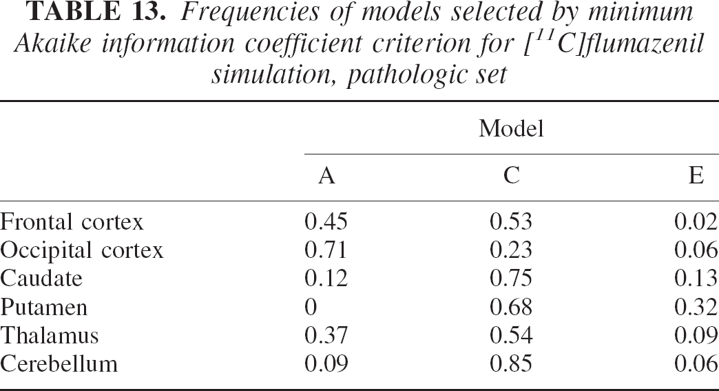
The results of this simulation are shown in the usual terms of bias, standard deviation, and MSE in Tables 10, 11, and 12. Table 13 shows frequencies of models selected by the minimum Akaike procedure. Table 14 shows the average weights for the AICc-weighted procedure.
Volume of distribution: bias for [11C]flumazenil simulation, pathologic set
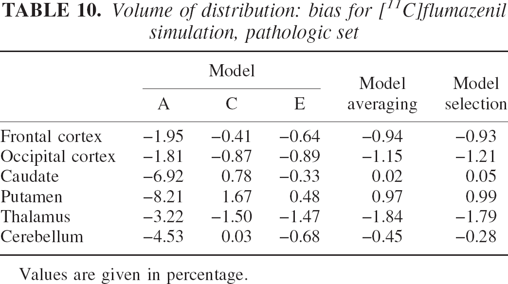
Values are given in percentage.
Volume of distribution: standard deviation for [11C]flumazenil simulation, pathologic set
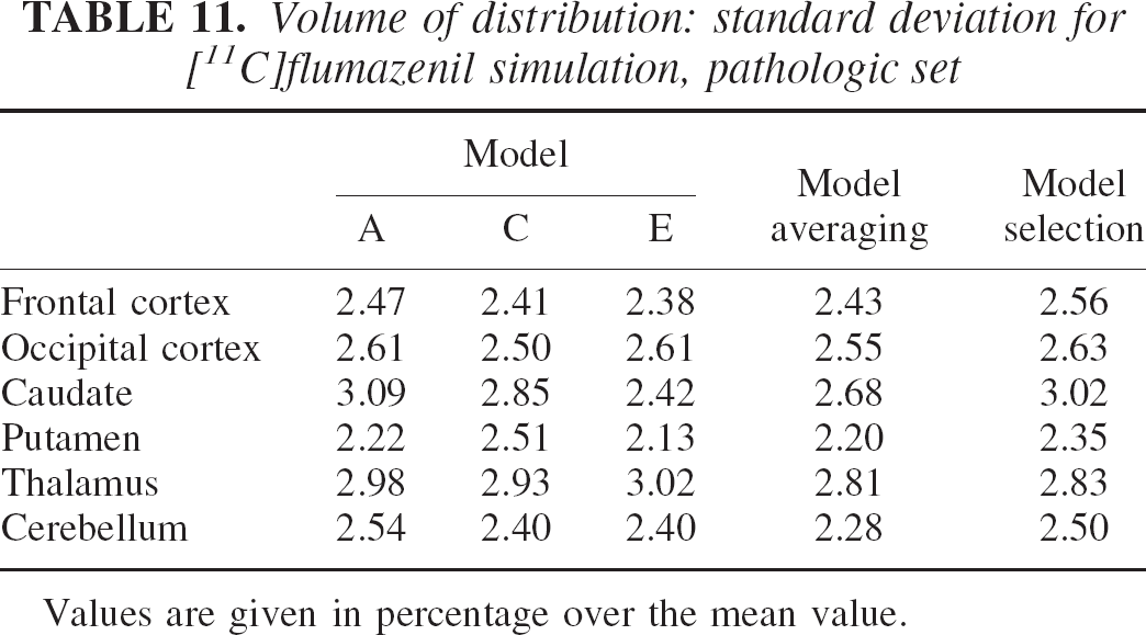
Values are given in percentage over the mean value.
Volume of distribution: mean squared error for [11C]flumazenil simulation, pathologic set
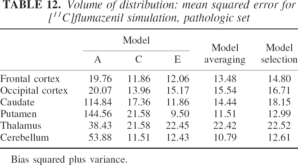
Bias squared plus variance.
Frequencies of models selected by minimum Akaike information coefficient criterion for [11C]flumazenil simulation, pathologic set
Mean values for Akaike weights for [11C]flumazenil simulation, pathologic set
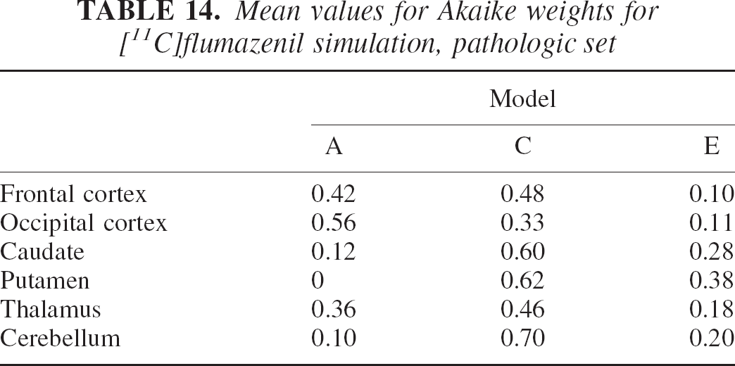
Table 12 shows that the reduction in specific uptake induced greater MSE owing to the relative increase of the nonspecific compartment contribution that is not considered by any of the three models used. As before, model averaging performed better than model selection in MSE terms over all regions. Table 14 illustrates how weights in the more complex models, C and E, have gradually increased to compensate for the change in kinetic properties of the system. Remember, however, that the model selected in the “normal” set was model A. Model A performance on the “pathologic set” is obviously degraded with an almost doubled increase in MSE compared with the model averaging method. Note that on this set, the model selected by the minimum AIC procedure was model C also for the frontal cortex (see Table 13).
DISCUSSION
The results contained in the experimental section, for real or simulated data, allow the following inferences. First, reality is complex and although no optimal model exists, better ones do. The distance of a model from the true data-generating mechanism can be calculated from its mean likelihood, and AIC coefficients are good estimates of this distance. Second, there may be instances where different models in a set may have comparable likelihood over the same data set. In this case, rejection of a model may cause more harm than good, and better estimates can be obtained by averaging the parameter of interest over the entire model set. The limitation is that all models must allow the estimation of the parameter of interest. Third, rejection of models can be even more harmful when one considers the generalization error, the error incurred when the model selected is applied on different data sets. Obviously, there will also be instances where model uncertainty will be low, and in this case model averaging will be reduced to the use of a single robust model. Finally, a method that allows the use of an array of models is a strong conceptual tool. For example, when physiologically appropriate, one could conceive the simultaneous use of blood and reference inputs to improve the statistical properties of the estimates. Furthermore, one could adapt more efficiently model complexity to varying spatial scales. This concept applies to the varying size of ROIs, as illustrated in the experimental section, but it could be also extended to multiscale approaches for the production of parametric maps (Turkheimer et al., 2000). These are among the possibilities that will be explored in future work.
Footnotes
Acknowledgments:
The authors would like to thank Kathy Schmidt (NIMH, Bethesda, MD, U.S.A.) for reading the manuscript and providing useful comments.