Sage Journals: Discover world-class research

Abstract

The construction of parametric positron emission tomography images of enzyme or receptor concentration obtained using irreversibly binding radiotracers presents problems not usually encountered with reversibly binding radiotracers. Difficulties are most apparent in brain regions having low blood flow and/or high enzyme or receptor concentration and are exacerbated with noisy data. This is especially true when minimal doses of radiotracer are administered. A comparison was recently reported of the irreversible monoamine oxidase A (MAO A) radiotracers [¹¹C]clorgyline (CLG) and deuterium-substituted [¹¹C]clorgyline (CLG-D) in the human brain using region of interest (ROI) analysis in which the authors observed an unexpected loss of image contrast with CLG-D compared with CLG. In order to more fully investigate patterns of binding of these irreversibly binding radiotracers, a strategy was devised to reduce noise in the generation of parametric images of the model term related to enzyme or receptor concentration. The generalized linear least squares (GLLS) method of Feng et al. (1995), a rapid linear method that is unbiased, was used for image-wide parameter estimation. Since GLLS can fail in the presence of large amounts of noise, local voxels were grouped within the image to increase the signal, and the GLLS method was combined with the standard nonlinear estimation methods when necessary. Voxels were grouped together depending on their proximity and whether they fell within a specified range of the time-integrated image. It was assumed that voxels meeting both criteria are functionally related. Simulations reflecting varying enzyme concentrations were performed to assess precision and accuracy of parameter estimates in the presence of varying amounts of noise. Using this approach, images were generated of the combination parameter λk₃ (λ = K₁/ k₂, where K₁ and k₂ are plasma-to-tissue and tissue-to-plasma transport constants, respectively) that is related to enzyme concentration as well as images of the transport constant K₁ for individual subjects. Reasonably high-quality images of both K₁ and λk₃ were obtained for CLG and CLG-D for individual subjects even with low injected doses averaging 6 mCi. While there were no differences in the K₁ images, the λk₃ images revealed the loss of contrast previously reported for CLG-D using the ROI analysis. This method should be generalizable to other tracers and should facilitate the analysis of group differences.

Keywords

Monoamine oxidase PET Kinetic modeling Parametric images

The enzyme monoamine oxidase, which occurs in two forms, MAO A and MAO B, catalyzes the oxidative deamination of amines from endogenous and exogenous sources (Shih et al., 1999). The two subtypes occur in different types of cells in the brain, with MAO B occurring predominately in glial cells and serotonergic neurons while MAO A occurs in catecholaminergic neurons as well as in glial cells. From a medical viewpoint, these enzymes are of interest for, among other things, their ability to regulate chemical neurotransmitters. Drugs inhibiting MAO have been used in the treatment of depression and Parkinson's disease. Two ¹¹C-labeled positron emission tomography (PET) tracers have been used for imaging MAO: L-deprenyl (MAO B) and clorgyline (MAO A). Both of these compounds are irreversible inhibitors of MAO. They bind covalently to the enzyme, which also inactivates it. This binding also traps the ¹¹C at the site of inactivation. While the graphical method of Patlak et al. (1985) is applicable to such irreversibly binding tracers and much easier to apply than compartment models, the influx constant, Ki, resulting from the Patlak analysis is a function of blood flow as well as the enzyme concentration, and both vary from one brain region to another. It is therefore necessary to separately evaluate the transport constants and model parameter related to enzyme concentration using some form of compartmental modeling. Another complicating factor is that tracer uptake for irreversible ligands is less sensitive to variations in enzyme level in brain regions having low blood flow and/or high enzyme concentration. In addition, parameter estimation is more difficult in the presence of noise, which is a greater problem in the construction of parametric images than in region of interest (ROI) analysis. Owing to the widespread distribution of MAO in the brain, it is advantageous to have an image map of the enzyme concentration, so these difficulties need to be addressed.

We report here a method for the construction and comparison of parametric images of MAO A in the human brain using [¹¹C]clorgyline (CLG) and deuterium-substituted [¹¹C]clorgyline (CLG-D). Deuterium substitution serves as a mechanistic tool for the investigation of the biochemical basis of the PET image. In the irreversible inhibition of MAO by CLG, the C-H bond on the methylene carbon of the propargyl group is cleaved in the rate-limiting step. When deuterium is substituted for hydrogen, the bond is more difficult to cleave and the rate of reaction is reduced, providing evidence that MAO catalysis is responsible for the irreversible trapping of C-11 in brain. We undertook this study in order to more thoroughly investigate unexpected differences in the magnitude of the deuterium isotope effect in different brain regions when these two tracers were compared using the ROI analysis (Fowler et al., 2001).

Two of the most important limiting factors for consideration in the construction of parametric images for CLG and CLG-D are (1) the signal-to-noise ratio at the voxel level and (2) the time involved in the parameter estimation process, which involves several thousand voxels per plane. The generalized least squares (GLLS) method is sufficiently rapid that images can be generated in a reasonable amount of time: on the order of minutes. It is, however, more sensitive to noise than the standard nonlinear estimation procedures. Low signal-to-noise ratio is a particular problem in the present study because the injected doses were low (6 to 7 mCi) in order to permit multiple studies in the same subject. In this study we compare, using computer simulations, the GLLS and nonlinear least squares (NLS) methods for the two-tissue compartment irreversible model in the presence of varying amounts of noise. Simulations reflecting varying enzyme concentrations were performed to assess precision and accuracy of parameter estimates. Results from the simulations indicate that the preferred model parameter for enzyme concentration is the combination parameter λk₃ as opposed to k₃ (λ = K₁/k₂, where K₁ and k₂ are plasma-to-tissue and tissue-to-plasma transport constants, respectively, and k₃ is the model parameter directly proportional to enzyme concentration). Unlike K₁ and k₂, λ does not depend on blood flow.

THEORY

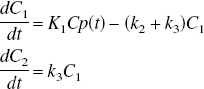
The uptake and binding of irreversible tracers such as CLG and [¹¹C]L-deprenyl can be described by the two-tissue compartment model with three model parameters, K₁, k₂ and k₃:

\begin{array}{l} C p \begin{array}{l} K_{1} \\ ⇄ \\ k_{2} \end{array} C_{1} \begin{array}{l} k_{3} \\ \to \end{array} C_{2} \\ Blood Brain \end{array}

which is a simplification of what is thought to be a multistep inactivation process (see Fowler et al., 1988, for a complete description of the model and simplifications). K₁ and k₂ are transport constants, both of which are functions of blood flow. The model parameter k₃ contains the enzyme concentration (E) so that k₃ = k₃′E. The enzyme concentration varies from one brain region to another, while the rate constant for inactivation, k₃′, is constant. C₂ is the concentration of tracer irreversibly bound to enzyme, and C₁ is tracer in brain tissue not irreversibly bound to enzyme. The plasma concentration of unmetabolized tracer is C_p. PET measures the total tissue radioactivity given by C₁ + C₂ plus a blood volume contribution. The differential equations corresponding to this model are

\begin{array}{l} \frac{d C_{1}}{d t} & = & K_{1} C p (t) - (k_{2} + k_{3}) C_{1} \\ \frac{d C_{2}}{d t} & = & k_{3} C_{1} \end{array}

(1)

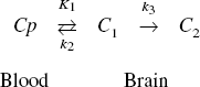
Analysis based on the direct application of these equations will be referred to as the nonlinear least squares (NLS) method. There is also a nonspecific binding component, which is assumed to be sufficiently rapid that it is incorporated into the model constants k₂ and k₃ (Mintun et al., 1984). With this assumption, the free ligand is a constant fraction of the free plus nonspecifically bound.

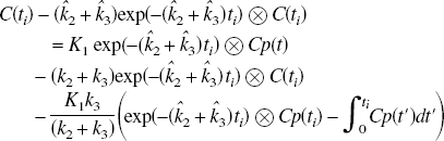
These equations can be solved explicitly through Laplace transform or numerically. The problem is to optimize the model parameters, which in this formulation requires an iterative solution using, for example, the Levenberg-Marquardt or Simplex methods (Press et al., 1990). These equations can also be written in a linearized form as (Blomqvist, 1984)

\begin{array}{l} C (t_{i}) & = & K_{1} \int_{0}^{t_{i}} C p (t^{'}) d t^{'} + K_{1} k_{3} \int_{0}^{t_{i}} \int_{0}^{t^{'}} C p (t^{″}) d t^{″} d t^{'} \\ - (k_{2} + k_{3}) \int_{0}^{t_{i}} C (t^{'}) d t^{'} \end{array}

(2)

which form a set of equations for tissue concentration/radioactivity designated by C(t_i) at discrete time points t_i. In this case, the optimum parameter values are determined by a linear least-squares solution of the set of simultaneous equations in Eq. 2. Analysis based on Eq. 2 will be referred to as the LLS method. This solution represents a considerable savings in calculation time over that of the iterative NLS method. The equation errors in the LLS solution are not independent, however, and as a result the parameter estimates from this procedure will be biased in the presence of noise (Feng et al., 1996). The generalized least-squares (GLLS) version of these equations developed by Feng et al. (1995) is

\begin{array}{l} C (t_{i}) & - & ({\hat{k}}_{2} + {\hat{k}}_{3}) exp (- ({\hat{k}}_{2} + {\hat{k}}_{3}) t_{i}) \otimes C (t_{i}) \\ = K_{1} exp (- ({\hat{k}}_{2} + {\hat{k}}_{3}) t_{i}) \otimes C p (t) \\ - & (k_{2} + k_{3}) exp (- ({\hat{k}}_{2} + {\hat{k}}_{3}) t_{i}) \otimes C (t_{i}) \\ - & \frac{K_{1} k_{3}}{(k_{2} + k_{3})} (exp (- ({\hat{k}}_{2} + {\hat{k}}_{3}) t_{i}) \otimes C p (t_{i}) - \int_{0}^{t_{i}} C p (t^{'}) d t^{'}) \end{array}

(3)

where ⊗ refers to convolution. This method provides unbiased parameter estimates. The equations are solved for the linear coefficients on the right hand side, K₁,(k₂ + k₃) and K₁k₃/(k₂ + k₃). An initial guess for k₂ + k₃ is required, and this method, like the NLS method, is iterative; convergence occurs in a few iterations, however, so it is more efficient than the NLS method.

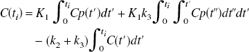
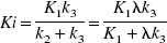
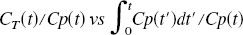
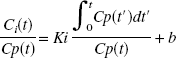
The ability to accurately estimate k₃ has been found to depend on its value relative to the efflux constant k₂ (Koeppe et al., 1996, 1999). When k₃ » k₂ (λk₃ » K₁), uptake depends primarily on K₁ and is relatively insensitive to changes in k₃ (uptake is flow limited). This can also be expressed in terms of Ki, which depends on K₁ and λk₃ (Ki = K₁k₃/(k₂ + k₃) = K₁λk₃/(K₁ + λk₃), where λ = K₁/k₂) as shown in Fig. 1A. Ki is used as a measure of uptake. Ki can also be obtained from a Patlak analysis (Patlak and Blasberg, 1985; Patlak et al., 1983) in which a plot of

C_{T} (t) / C p (t) v s \int_{0}^{t} C p (t^{'}) d t^{'} / C p (t)

becomes constant after some time t* with a slope given by Ki. C_T(t) is tissue radioactivity at time t. Figure 1A is a plot of Ki versus λk₃ for K₁ values of 0.25, 0.50, 0.75, and 1.0 mL/g/min with the maximum value λk₃ = 3.0. The flow-limited nature of the uptake is indicated when Ki changes very little with changes in λk₃. For K₁ = 0.25, sensitivity is greatly reduced for λk₃ > 0.75. With larger values of K₁, Ki is sensitive to changes in λk₃ over a much wider range. The values most relevant to clorgyline are indicated by the dotted line in Fig. 1B, with K₁ between 0.25 and 0.5 mL · g⁻¹ · min⁻¹

FIG. 1. (A)

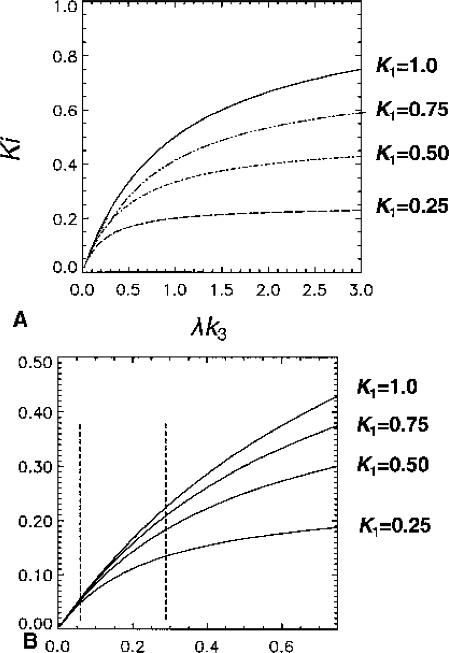
A plot of Ki versus λk₃ for K₁ values of 0.25, 0.50, 0.75, and 1.0 mL · g⁻¹ · min⁻¹. The flow-limited nature of the uptake is indicated when Ki changes very little with changes in λk₃. (B) Ki versus λk₃ over a range of λk₃ for which uptake is reasonably sensitive to variations in enzyme level. Values that span the range for clorgyline are indicated by the dashed lines. For clorgyline, K₁ values are between 0.25 and 0.5 mL · g⁻¹ · min⁻¹, which are less than those of deprenyl, which are generally between 0.5 and 1.0.

MATERIALS AND METHODS

Computations

Solution of the differential equations Eq. 1 and optimization of model parameters were accomplished using routines in Numerical Recipes in C (Press et al., 1990). Numerical integrations in Eqs. 2, 3, and 5 were performed using the routine “qtrap” also from Numerical Recipe in C. A linear interpolation between time points was used for the concentration values associated with frame mid times for both ROIs and voxel approaches. Equal weights were used in all of the linear analyses. Parameter estimation for the NLS method was accomplished using a simplex method.

Simulations

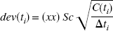
Solution of the irreversible three-compartment model with the GLLS method was tested with simulations using transport constants K₁ and k₂ fixed at 0.31 mL · g⁻¹ · min⁻¹ and 0.085 min⁻¹, respectively (typical of those found for CLG and CLG-D). Values of k₃ used were 0.008, 0.012, 0.055, 0.08, and 0.20 min⁻¹ to represent the spread of values over different regions applicable to both H/D clorgyline and H/D deprenyl. A measured CLG input function was used to generate the data using Eq. 1. Additive noise (dev) to simulate counting statistics based on ¹¹C was generated using pseudo random numbers (xx) from a gaussian distribution with 0 mean and variance of 1.

d e v (t_{i}) = (x x) S c \sqrt{\frac{C (t_{i})}{Δ t_{i}}}

(4)

Sc is a scale factor that determines the level of noise, Δt_i is the scan length, and C(t_i) tissue radioactivity at time t_i. Values used for Sc were 4, 2, and 1, ranging from a very high noise level (Sc = 4) to a low noise level (Sc = 1). At each noise level, 500 data sets were generated. Time points from t = 1 minute were used in the fitting process. The failure rate of the GLLS method increases with increasing noise. When it fails (provides negative values or the parameters exceed specified limits), the differential equations are solved directly using the NLS method but fixing the ratio λ = K₁/k₂ so that only two model parameters need to be determined.

Positron emission tomography studies

Preparation of CLG and CLG-D have been described previously (Fowler et al., 2001; MacGregor et al., 1988). PET scans were run on a whole body, high-resolution positron emission tomograph (Siemen's HR+ 4.5 × 4.5 × 4.8 mm at center of field of view) in 3D dynamic acquisition mode. Experimental details have been described (Fowler et al., 2001) and data reported here are from the five subjects used in those studies. Plasma samples were analyzed for CLG (or CLG-D) using the same solid phase extraction procedure described previously for deuterated [¹¹C]L-deprenyl (Alexoff et al., 1995).

Parametric image generation

Image registration. For each subject, the CLG and CLG-D images were summed over time frames and coregistered using the SPM software (SPM software MRC Cyclotron Unit, Hammersmith Hospital, London, 1995). Spatial normalization parameters were obtained from the subject means of the two coregistered images in order to map the images to the Talairach atlas. The transformation parameters were applied to each time frame for the H and D scans of each subject. Planes were added in groups of two, placing the thalamus at plane 12, to obtain 23 planes. Images were registered to the Talairach atlas (Talairach and Tournoux, 1988).

Signal enhancement. Before parameter estimation, a time-integrated image was formed and the maximum value was scaled to 100. Only integrated voxel values that exceeded a specified fraction of the maximum voxel value of the integrated image were treated as actual brain tissue and were used in the analysis. This value was determined by displaying the integrated image of each study for different cutoff values. Values between 20 and 25 were used for clorgyline. To further improve the signal-to-noise ratio, local voxel values were averaged at each time point according to two criteria: (1) that they are within ±n voxels of the voxel being analyzed, and (2) that the integrated voxel value within this region fall within a specified range of that of the voxel being calculated. These values were ±4 voxels and ±2.5% of the integrated voxel value. For lower integrated voxel values (<55), these were increased to ±5 and ±5%, respectively. A second scheme was tested in which the integrated voxel was divided into two parts: from 0 to 10 minutes and from 10 to 60 minutes. The reason for exploring the two-part integration was that this would ensure that voxels had similar blood flow (as determined by similarity in first part of the uptake) as well as similar enzyme levels as determined by the plateau (later time points). These two images were used in the same way, except that the two criteria were imposed on both. Both of these schemes have the effect of grouping voxels within a structure which have similar uptake without explicitly defining a region of interest. However, it differs from an ROI with a single value of uptake at each time point in that each voxel was calculated separately. The term SEV will be used to refer to single voxel calculations using the signal enhancing multivoxel averaging described here, and the term ROI will refer to results using the average of all voxels within an ROI at each time point. The term single voxel will refer to analysis on image voxels without any other processing.

Parameter estimates. Both the GLLS method and the direct solution of the differential equations require initial estimates for the model parameters. In many cases, an adequate initial guess is provided by the linearized equations (Blomqvist, 1984) given by Eq. 2. This gives a good estimate of K₁, but in the presence of significant noise it may not provide realistic values for k₂ and/or k₃. When k₂ or k₃ values are found to be negative or exceed some specified value (λ >8or λ < 0.75 were used as cutoff values), an alternative initial guess can generally be obtained from the Patlak analysis (Patlak and Blasberg, 1985; Patlak et al., 1983),

\frac{C_{i} (t)}{C p (t)} = K i \frac{\int_{0}^{t} C p (t^{'}) d t^{'}}{C p (t)} + b

(5)

which is linear with slope Ki for times t > t*. In terms of model parameters,

K i = \frac{K_{1} k_{3}}{k_{2} + k_{3}} = \frac{K_{1} λ k_{3}}{K_{1} + λ k_{3}}

and λ = K₁/k₂. Given K₁ from the linear analysis and Ki from the Patlak analysis, k₂ and k₃ can be estimated from Ki assuming a fixed value of λ obtained from a prior ROI analysis. Using these initial values, the GLLS method was applied. If this method failed (or k₂ or k₃ were found to be <0 or 0.75 > λ > 8 or λk₃/K₁ > 2.0), the NLS method with λ fixed was used for the parameter estimation (the GLLS-NLS method). If the NLS estimate of λk₃/K₁ exceeded 2.0, a region of lower sensitivity (Fig. 1), the voxel value was determined in a postprocessing procedure by averaging λk₃ values of local voxels.

Analysis of image differences between [¹¹C]clorgyline and deuterium-substituted [¹¹C]clorgyline

The properties of the CLG and CLG-D images were compared by first scaling the D images such that an ROI from the thalamus (ROI_TH) was constrained to have the same value for both the H and D studies, that is, by scaling the D image by the factor ROI_TH(H)/ROI_TH(D). The H and scaled D images were then compared for potential differences; however, owing to the correlation between voxels, the application of statistical tests requires modification since the true number of independent data points is unknown. A value for the number of independent points was selected by reducing the number of image voxels by a factor np. Values of np from 20 to 100 were used so that for N voxels, the number of data points in the evaluation of significance was taken to be N/np, which gives 330 and 70 (for np = 20 and 100, respectively) as the number of independent data points for the thalamus plane. Images at the level of the thalamus and cerebellum were compared for differences in mean using a t-test and for different variances by means of the F-test using the reduced number of degrees of freedom (Numerical Recipes in C).

RESULTS

Simulations

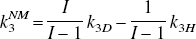
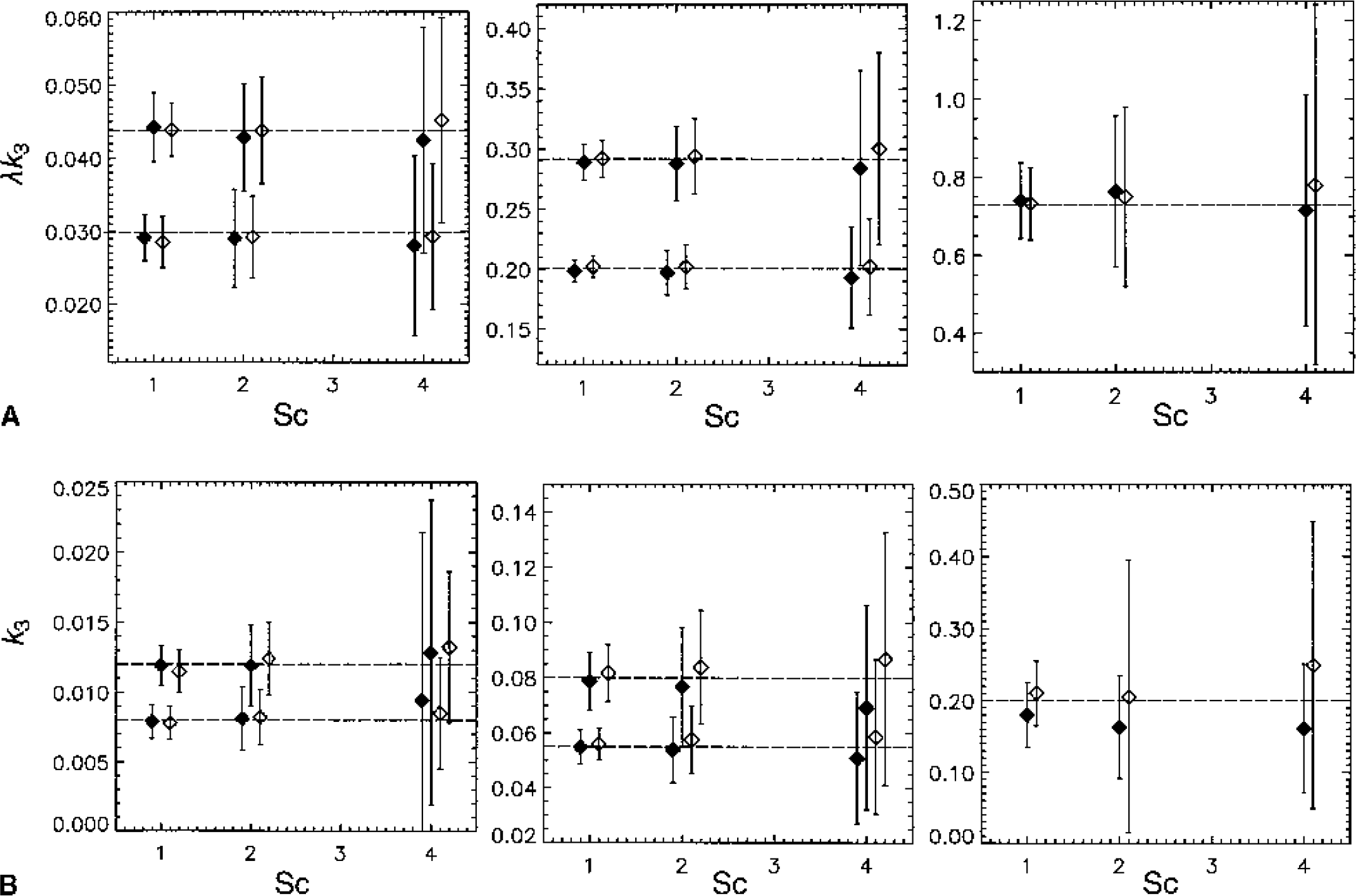
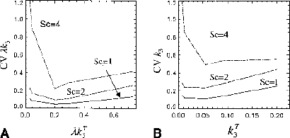
Results of the simulations (n = 500) are shown in Figs. 2, 3, and 4. Figure 2A gives average values and standard deviation (SD) for λk₃ versus noise level as determined by Sc values of 1, 2, and 4. Figure 2B gives results for k₃ versus noise level. For clarity, symbols are shown slightly displaced from the Sc value actually used. The true values (λk^T₃ and k^T₃) are indicated by the dashed lines. For λk^T₃ these are 0.029, 0.044, 0.20, 0.29, and 0.73 mL · g⁻¹ · min⁻¹ (corresponding to k^T₃ = 0.008, 0.012, 0.055, 0.08, 0.20 min⁻¹). The GLLS-NLS method slightly underestimates λk₃ at the highest noise levels. The mean values from both NLS and GLLS-NLS, however, differ from the true value by less than 5%. For k₃ there are larger differences; the GLLS-NLS method underestimates k₃ by 20% for Sc = 4 with k^T₃ = 0.20 min⁻¹. The NLS method tends to overestimate k₃ with increasing noise, while the GLLS-NLS method tends towards an underestimation. The coefficient of variation (CV) for λk₃ was less than for k₃ as expected (Figs. 3A and 3B, respectively). The smallest CV at all noise levels occurs for λk₃ = 0.20. The CVs were generally smaller for the NLS method except for Sc = 4 with k^T₃ = 0.20. The GLLS method failed for 20 of 500 (for k^T₃ = 0.008, Sc = 2), reverting to the NLS solution with λ fixed as described above. This number increased to 300 of 500 for k^T₃ = 0.20 (Sc = 4). As a result, the GLLS-NLS had a smaller SD (Fig. 2A) than the NLS method. This is due to the fact that when the GLLS method failed, the NLS method was implemented with λ fixed, thus reducing the number of parameters determined. Figure 4A shows the variation in mean value of λ with k^T₃ for Sc = 2 and Fig. 4B shows λ versus Sc for k^T₃ = 0.08 min⁻¹. λ deviates from the true value as k^T₃ increases (Fig. 4A) and the CV increases as well (0.86 for = 0.20). λ also increases with increasing noise (Sc) (Fig. 4B). On the other hand, K₁ estimates (Fig. 5) are only 3% below the true value when k^T₃ = 0.20 (Fig. 5). Parameter estimates of λ and k₃ are negatively correlated r = −0.91 for Sc = 1 and r = −0.10 for Sc = 4 (P < 0.0005) consistent with a positive correlation between k₂ and k₃.

FIG. 2. (A)

Average values and standard deviation (SD) for λk₃ versus noise level (Sc) for nonlinear least squares (NLS) and generalized linear least squares (GLLS-NLS) methods. For clarity, symbols are shown slightly displaced from the Sc value actually used. Values determined by the NLS method are indicated by ⋄ and by ⧫ for the GLLS-NLS method. The dashed line indicates the true values of λk^T₃, which were 0.029, 0.044, 0.20, 0.29, and 0.73. (B) Average values and SD for k₃ versus noise level for NLS and GLLS-NLS. The true values are indicated by the dashed lines. For k^T₃ these are 0.008, 0.012, 0.055, 0.08, and 0.20 min⁻¹.

FIG. 3. (A)

Coefficient of variation (CV) for λk₃ as a function of noise level (Sc) and λk^T₃ for the generalized linear least squares–nonlinear least squares (GLLS-NLS) method. (B) Coefficient of variation for k₃ as a function of noise level and k^T₃ for the GLLS-NLS method.

FIG. 4. (A)

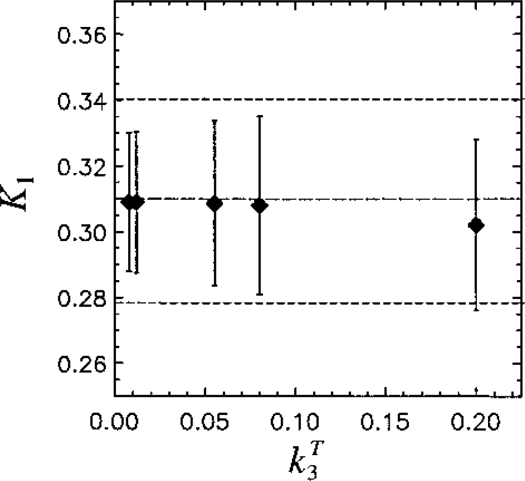
λ versus k^T₃ for one noise level (Sc = 2) for the generalized linear least squares–nonlinear least squares (GLLS-NLS) method. The estimated value of λ increases with increasing k^T₃. (B) λ versus noise level (Sc) for k^T₃ = 0.08 min⁻¹ for the GLLS-NLS method. The estimated value of λ increases with increasing noise.

FIG. 5.

K₁ versus k^T₃ for Sc = 2. Mean estimates of K₁ deviate only slightly from the true value, k^T₃,as k^T₃ increases.

Images

Parametric images of K₁ and λk₃ are shown in Fig. 6 for three of the five subjects. Two planes are shown: one at the level of the thalamus and one at the level of the cerebellum. The λk₃ images from CLG and CLG-D are displayed on the same scale by multiplying the deuterium images by the ratio of a thalamus region of interest for CLG to that of CLG-D for each subject. The λk₃ images for CLG-D show less contrast than those of CLG. The K₁ images are not scaled and are similar for both compounds with no loss of contrast in the D images. These images were generated by grouping voxels within a region of ±4 voxels and within 2.5% of the integrated image except in regions of low uptake. When the value of the scaled integrated images was <55, the acceptance was increased to ±5% to compensate for low counts. The average number of grouped voxels was in the range of 15 to 25. The number of voxels for which the NLS method was used varied considerably depending on the plane (related to count rate) and study. For example, planes at the level of the thalamus required the NLS method for −1.5% or less of the voxels while at level of the cerebellum this increased to 5% to 10%. Using the integrated image in two parts did not improve the image and required larger limits on number of voxels and acceptance region, ±5 voxels and 5.5%, respectively. The values with the two-part integration were within ±2% for the thalamus and cerebellum ROIs. The important point is that a sufficient number of voxels are required in order to generate reasonable λk₃ images, and this number is larger in regions of lower counts.

FIG. 6.

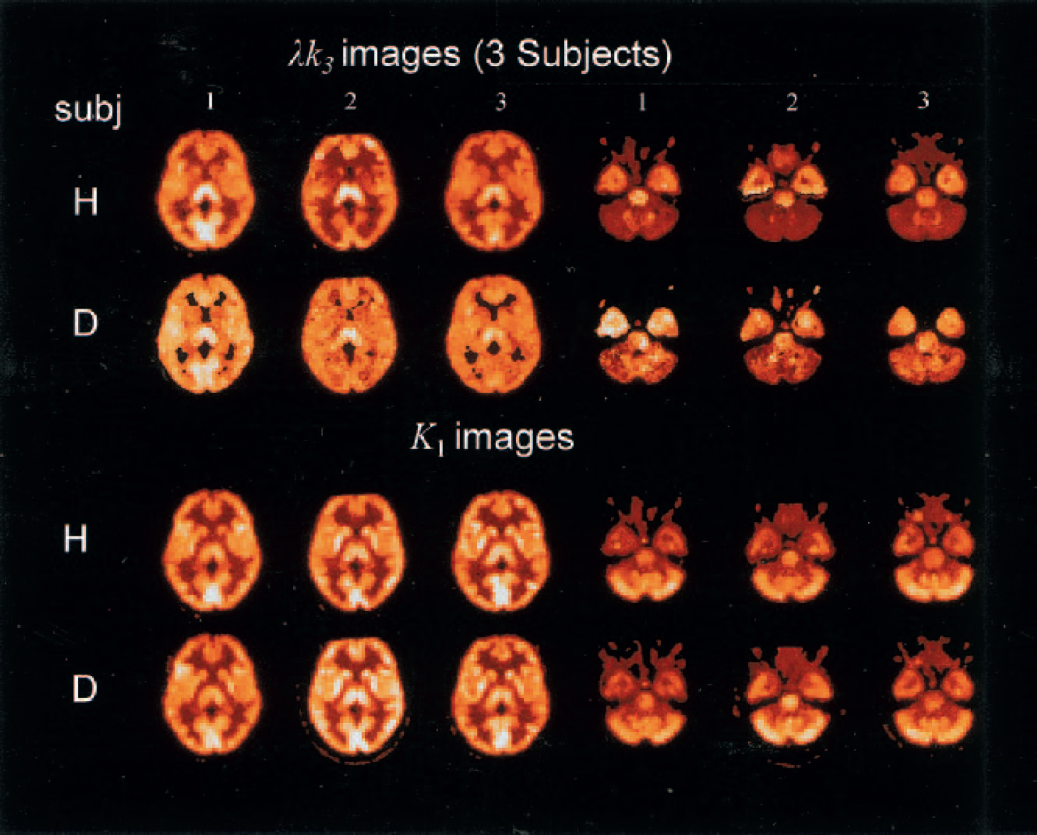
Parametric images of K₁ and λk₃ for three of the five subjects. Two planes are shown, one at the level of the thalamus (left) and one at the level of the cerebellum (right). The λk₃ images from [¹¹C]clorgyline (CLG) and deuterium-substituted [¹¹C]clorgyline (CLG-D) are displayed on the same scale bymultiplying the deuterium images by the ratio of a thalamus region of interest for CLG to that of CLG-D for each subject. The λk₃ images for CLG-D show less contrast than those of CLG. The K₁ images are not scaled and are similar for both compounds with no loss of contrast in the CLG-D images.

Figure 7 illustrates a histogram of the λk₃ values from the plane including the thalamus for all five subjects for the H and scaled D. The images were constrained to include the same number of voxels by using the same voxels from each image for which both exceeded a cutoff value. The average, median, and SD are given. The distribution of values in the thalamus (TH) plane appears to be broader for CLG than for the scaled CLG-D, which accounts for the greater contrast. For the cerebellum (CB; images on the right in Fig. 6) the distributions of λk₃ for CLG-D are similar in width but with a higher median and average values than for CLG (data not shown). A t-test on the difference in means between CLG and scaled CLG-D for the TH plane found a significant difference in all cases but 1 for np = 100 (df = 70, P < 0.05, t ranged from −4.1 to −2). For three of five subjects, the F-test for differences in variances found CLG distribution significantly greater than the scaled CLG-D for np = 100 (P < 0.005, F ranged from 2.1 to 1.4). For the CB plane, a significantly greater mean for scaled CLG-D occurred in four of 5 cases for np = 50 (df = 75, P < 0.05, t ranged from −6 to −2). There was a significantly greater variance for CLG in 3 of the 5 subjects for np = 50 (df = 75, P < 0.05, F = 1.5 for all 3). The average difference in mean between scaled CLG-D and CLG was greater for CB image than for TH image, 0.241 ± 0.18 (CB) and 0.095 ± 0.13 (TH). In contrast, no significant difference in mean or variance was found for H and D distributions of K₁ for np = 75.

FIG. 7.

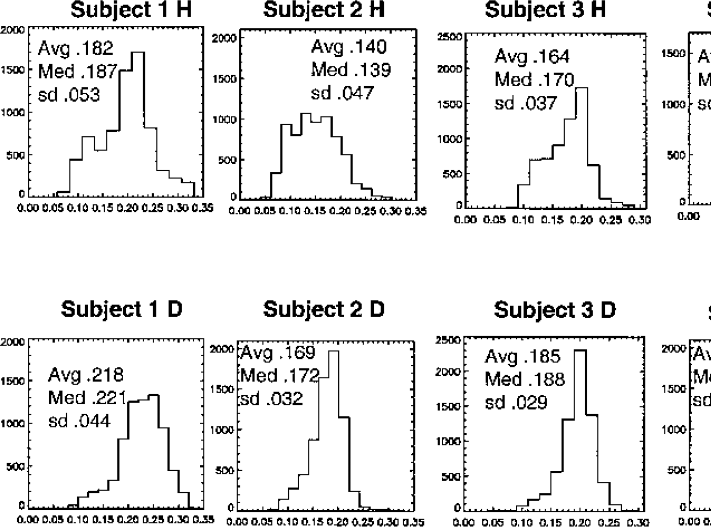
Histograms of λk₃ from a plane containing the thalamus for [¹¹C]clorgyline (CLG) and scaled deuterium-substituted [¹¹C]clorgyline (CLG-D) for all five subjects. Images were constrained to have the same number of voxels. Note the broader distribution of values for CLG than for CLG-D. The average (Avg), median (Med), and standard deviation (sd) are shown.

Figures 8A and 8B illustrate the average CV, determined from the average and SD of voxels from the thalamus and cerebellum regions, for λk₃ and k₃ over all five subjects. Calculations of λk₃ and k₃ used both the SEV (the signal-enhanced voxel) and single voxel methods. The GLLS-NLS estimation method was used for both the SEV and single voxel, and for comparison the single voxel NLS estimation was also included. The average value from the SEV method (data not shown) was in good agreement with the traditional ROI value (using NLS). The CVs were considerably less for the SEV calculation of Xk₃ compared with the single voxel calculation (P < 0.05, paired t-test). The CV for CLG was less than that for CLG-D and the CV for thalamus was less than that for cerebellum. For k₃, the SEV CVs are considerable greater than for λk₃ (P < 0.05, paired t-test). For CB using the single voxel GLLS-NLS method, the average value for λk₃ was 6% less than that calculated using the ROI method for CLG-D and 4% less for CLG. For THL, the GLLS-NLS single voxel method was 3% less for CLG-D, with no difference found for CLG.

FIG. 8. (A)

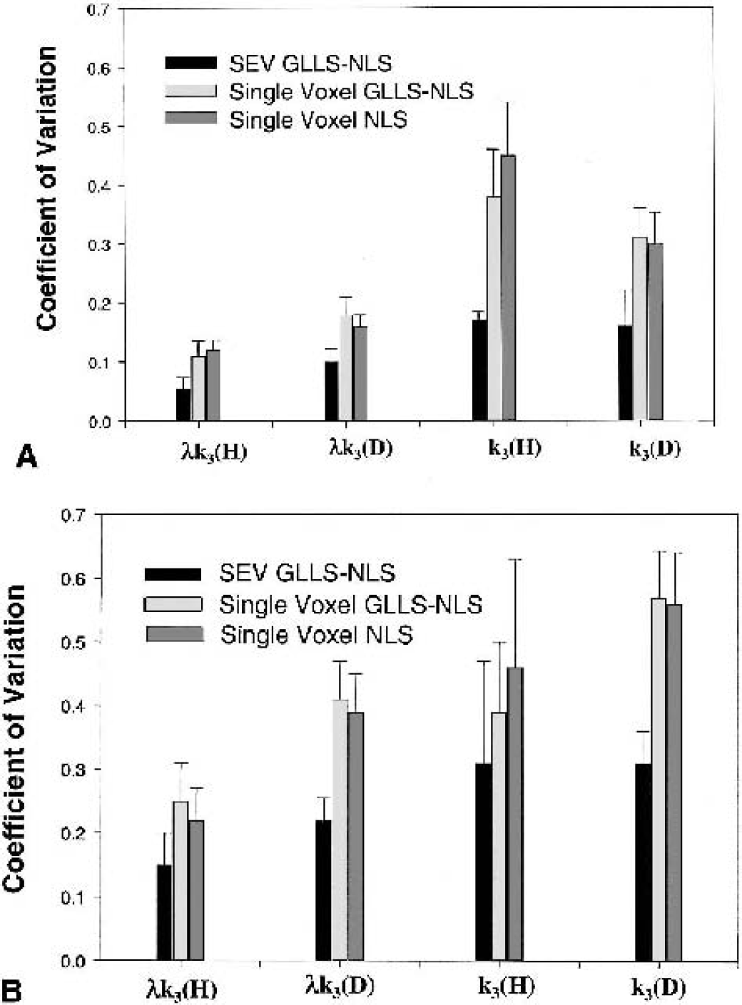
Coefficient of variation (CV) of λk₃ and k₃ from the thalamus region for the signal-enhanced voxel (SEV) and single voxel methods. The SEV method refers to the signal enhancement procedure applied to each voxel in the defined region of interest. The generalized linear least squares-nonlinear least squares (GLLS-NLS) method was used. For comparison, the CV from calculations based on a single voxel approach (no enhancement) for both GLLS-NLS and NLS are also presented. The average value for the thalamus region using the SEV method (data not shown) was in good agreement with the traditional ROI value. The CVs were considerably less for the SEV calculation of λk₃, with the CV for CLG less than that for CLG-D. For k₃ the CVs are considerable greater than for λk₃. 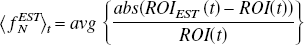(B) Coefficient of variation of λk₃ and k₃ from the cerebellum region for the SEV and single voxel methods. Using the single voxel GLLS-NLS method, the average value for λk₃ was 6% less than that calculated using the ROI method for CLG-D and 4% less for CLG. The CVs were considerably less for the SEV calculation of λk₃ compared with the single voxel GLLS-NLS or NLS methods, with the CV for CLG less than that for CLG-D. For k₃ the CVs are considerable greater than for λk₃ for all three.

Although it is not possible to directly relate the noise level in these images to that used in the simulations, a comparison of the quantity (averaged over time points t) given by

{〈 f_{N}^{E S T} 〉}_{t} = a v g {\frac{a b s (R O I_{E S T} (t) - R O I (t))}{R O I (t)}}

(6)

where ROI(t) is the data and ROI_EST(t) is the value generated by the model, can be used to relate the simulations to the image data. For the single voxel, GLLS-NLS analysis of the image regions from thalamus and cerebellum is 0.10. For simulation data, the values for Sc = 4, 2, and 1 were, respectively, 0.3, 0.1, and 0.05, which would place the image data in the vicinity of Sc = 2.

DISCUSSION

The simulation results indicate that the accurate estimation of the enzyme parameter depends on multiple factors. One factor is the amount of tracer in the tissue and the half-life of the isotope. Another is the sensitivity of the uptake curve to variations in the amount of enzyme, as illustrated in Fig. 1. The greatest sensitivity occurs for lower values of enzyme, but accuracy of parameter estimation is also dependent on having sufficient tracer in tissue to achieve a signal. The largest CVs were obtained for the lowest values of k₃ (Fig. 3) at the highest noise level. At the high end when λk₃ » K₁ (or equivalently k₃ » k₂), uptake depends primarily on K₁ and is relatively insensitive to changes in k₃ or λk₃, (the “flow-limited” case). The largest value of λk₃ used in the simulations was 0.73 (k₃/k₂ = λk₃/K₁ = 2.4). From Fig. 1 this region is of lower sensitivity than λk₃ = 0.20. This places some limits on the range of enzyme concentration that a particular tracer can accurately estimate. For deprenyl, K₁ has values close to what would be expected for blood flow (0.60 mL · g⁻¹ · min⁻¹), and λk₃ is on the order of 0.5 (white matter) to 2.0 or greater in thalamus, which is a region of lower sensitivity since λk₃/K₁ = 3.3 (Fig. 1A). The introduction of the deuterium (D deprenyl) reduces λk₃ so that the maximum values are on the order of 0.4 to 0.5 with minimum values in the range 0.12, which puts λk₃ in a region of greater sensitivity since λk₃/K₁ < 1 (Fig. 1B). For CLG the λk₃/K₁ ratio is on the order of 0.8 for thalamus and 0.45 for cerebellum. For CLG-D these ratios are 0.25 and 0.17 for thalamus and cerebellum, respectively. Koeppe et al. (1999) report that optimum values of λk₃/K₁ for the accurate estimation of k₃ range from 0.1 to 0.3. From our simulations, the optimum value was 0.6 for k₃ = 0.055 (λk₃ = 0.20), for which the CVs for both λk₃ and k₃ go through a minimum (Fig. 3). The true minimum may actually occur between the values k₃ = 0.055 and 0.012 (corresponding to λk₃/K₁ = 0.14). For larger values of λk₃/K₁, the effect of noise on parameter estimation is much greater. Note the larger CVs for λk3 = 0.73 (λk₃/K₁ = 2.35) than for λk₃ = 0.20. Also at higher noise levels and larger values of k^T₃, the accurate estimation of k₂ and k₃ is much more difficult. As illustrated in Fig. 4A, there is a positive correlation between λ and k^T₃ (Sc = 2) so that the average value of λ increases with increasing k^T₃. The CV estimates of λ also increase with noise when k^T₃ is held constant. K₁ values, on the other hand, show only a small decrease (<5%) as k^T₃ increases (Fig. 5). The combination parameter λk₃ eliminates this correlation problem.

The range of values found for λk₃ previously reported for deprenyl (Fowler et al., 1995) seem to be consistent with experimental measurements of MAO B from postmortem studies. Ratios of between 2.5 and 3 were estimated for the thalamus-to-cerebellum and basal-ganglia-to-cerebellum ratios (Fowler et al., 1995) based on data from Fowler et al. (1980), Glover et al. (1980), and Oreland et al. (1983). Values for MAO A appear to be in the same range. In comparison, a much greater difference is seen for the enzyme acetylcholinesterase (AchE), for which the experimentally measured trapping rates differ by 20 to 30 between the highest and lowest regions (Atack, 1986; Reinikainen et al., 1988). Koeppe et al. (1999) used the tracer PMP to measure AchE levels and found that the range of values across regions for k₃ depended on the method used in the estimation procedure, a result of the loss of sensitivity at higher enzyme levels. An unconstrained procedure for estimating all three parameters gave estimates for the range of k₃ values far lower than a constrained estimation in which k₃ was calculated as λk₃/4. This assumes that the true value of λ is 4 and constant across the brain. This last procedure is analogous to the use of the combination parameter λk₃. The unconstrained procedure underestimated k₃ in regions of high enzyme activity, whereas the constrained procedures gave values much closer to the reported range of enzyme activity, which lends support for the use of λk₃ over k₃.

Parametric images of k₃ for CLG and CLG-D, in addition to being considerably more noisy than images of λk₃, do not show the higher enzyme level characteristic of the MAO A in the thalamus, most likely because of the correlation problem between k₂ and k₃ (and the amount of noise since the ROI data show a greater amount of binding in thalamus). Aside from eliminating the correlation problem, a second reason for using λk₃ is that it does not depend on nonspecific binding. Since the nonspecific binding is incorporated into the constants k₂ and k₃, the dependence of λk₃ on nonspecific binding has been removed since it appears in both k₂ and k₃ and therefore cancels (Carson et al., 1997). However, λk₃ is dependent on plasma protein binding (which is also rapid, similar to nonspecific binding) through K₁. There is some indication that λ is somewhat larger for CLG-D than for CLG. Using a global ROI λ_D is greater than λ_H with an average ratio of 1.15 (D/H). Also λ for CB is somewhat larger than for TH (based on ROI data from Fowler et al., 2001) for CLG-D. The average ratio is 1.12 (CB/TH). For CLG the difference is less. These regional differences may be due to small differences in nonspecific binding, in which case λk₃ is a better measure, since it does not depend on nonspecific binding.

Since the λk₃/K₁ ratios for CLG and CLG-D appear to be fairly close to the optimal range, this ensures adequate sensitivity of the model parameters to variations in enzyme level. The other factor contributing to the quality of the images is the noise associated with low counting statistics at the voxel level. Based on the simulations, the accuracy of parameter estimation and coefficients of variation of the values are improved by a reduction in noise. Also, because the GLLS method is a linear method, it is more sensitive to noise than the NLS method. The strategy of combining local voxels based on proximity and whether they fall within a specified range of the integrated voxel value improves the counting statistics. Furthermore, by meeting both criteria, the assumption is that the grouped voxels are likely to be functionally related. Although this will tend to smear out the signal, it reduces noise. Voxel grouping, along with the combination of the GLLS method with the NLS method as described, allows the rapid generation of reasonably good-quality images of the model parameters λk₃ and K₁, even though the injected radioactivity averaged only 6 to 7 mCi. For comparison, Koeppe et al. (1999) injected 16 to 32 mCi when studying the irreversible tracer [¹¹C]PMP. Other strategies have been used for grouping voxels in order to improve the signal; for example, Kimura et al. (1999) have used a cluster analysis procedure averaging over voxels with similar concentration histories in a two-parameter model.

Figure 6 illustrates the loss of contrast in the CLG-D λk₃ images compared with the CLG images. This is presumably due to a slow nonspecific binding component that cannot be separately evaluated apart from the MAO A binding and that is not diminished with D substitution. A rapid nonspecific binding component would be incorporated into the parameters λ (in k₂) and k₃ as the nonspecific binding fraction. In that case, it would not enter into λk₃. The fact that λ is slightly higher for CLG-D would be consistent with a small increase in the rapid nonspecific binding. In spite of the fact that the images appear different, SPM analysis (SPM software MRC Cyclotron Unit, Hammersmith Hospital, London, 1995) of the two groups, the CLG versus the scaled CLG-D, did not find specific areas of significant difference, although differences were detected in the ROI analysis. As an alternative means of comparing the CLG and CLG-D images, histograms of λk₃ values corresponding to planes at the level of TH and CB were used. The histograms of Fig. 7 for CLG and scaled CLG-D images illustrate the generally broader distribution of λk₃ for the CLG images at the plane including the thalamus. The broader distribution is consistent with the increased contrast, whereas the CLG-D distributions are more peaked and narrower, consistent with a smaller range of values, and therefore have less contrast. For subjects 1, 2, and 3, the variance of the CLG distribution was significantly greater than for the scaled CLG-D distribution for a reduction factor (np) of 75 for which there would be 90 independent data points in the image (there are on the order of 7,000 voxels per image). The difference in variance is less for subjects 4 and 5. In general, subjects 1, 2, and 3 showed greater differences between CLG and CLG-D images than subjects 4 and 5. Also, the mean for the scaled CLG-D image is greater than for the CLG image in all subjects except 4. Since the scaling was based on the thalamus, which is one of the regions with the greatest amount of MAO A, this indicates that the reduction in binding for other regions is less. Similarly for the cerebellum plane, the scaled CLG-D distributions have larger averages than the CLG. In comparison, there is no significant difference in variance for the K₁ images for any of the five subjects.

There is some question as to whether this additional binding is uniform. It certainly forms a larger fraction of the binding in the cerebellum (and white matter) than in the thalamus, which has a greater amount of MAO A. The relative contributions can only be calculated if the true isotope reduction factor is known. The non-MAO contribution can be calculated as (Fowler et al., 2001)

k_{3}^{N M} = \frac{I}{I - 1} k_{3 D} - \frac{1}{I - 1} k_{3 H}

(7)

where I is the isotope reduction factor [k₃(H)/k₃(D)]. For example, for I = 4, the non-MAO A contribution is similar in CB and TH for subjects 1, 2, and 3.

The nonuniform reduction in binding reported here was first observed visually on the time-summed images and confirmed in a ROI analysis of the data. In this work we have extended the analysis to parametric images of λk₃ and analyzed differences in the distribution of values of the model parameter in two planes involving the thalamus and the cerebellum. This required developing a technique to increase the signal-to-noise ratio in these experiments with low injected radioactivity. The simple strategy of combining local voxels with similar integrated activity increased the signal and allowed the use of the GLLS method. When the GLLS method failed, the NLS method with λ fixed was used. This occurred more frequently in regions of low uptake. Taken together, these procedures allowed the generation of images of the combination parameter λk₃, which is a measure of enzyme concentration.

Footnotes

Acknowledgments:

The authors thank Robert Carciello, Colleen Shea, Robert MacGregor, Victor Garza, Donald Warner, Noelwah Netusil, and Pauline Carter for advice and assistance in performing these studies. We also thank the people who volunteered for these studies.

References

Alexoff

Shea

Fowler

King

Gatley

Schlyer

Wolf

(1995) Plasma input function determination for PET using a commercial laboratory robot. Nucl Med Biol 22:893–904

Atack

Perry

Bonham

Candy

Perry

(1986) Molecular forms of acetylcholinesterase and butyrylcholinesterase in the aged human central nervous system. J Neurochem 47:263–277

Blomqvist

(1984) On the construction of functional maps in positron emission tomography. J Cereb Blood Flow Metab 4:629–632

Carson

Breier

de Bartolomeis

Saunders

Schmall

Der

Pickar

Eckelman

(1997) Quantification of amphetamine-induced changes in [11C]raclopride binding with continuous infusion. J Cereb Blood Flow Metab 17:437–447

Feng

Chen

L-C

Wang

J-K

Liu

R-S

Yeh

S-H

(1995) An evaluation of the algorithms for determining local cerebral metabolic rates of glucose using positron emission tomography dynamic data. IEEE Trans Med Imag IEEE 14:697–710

Feng

Huang

S-C

Wang

(1996) an unbiased parametric imaging algorithm for nonuniformly sampled biomedical system parameter estimation. IEEE Trans Med Imag 15:512–518

Fowler

Wiberg

Oreland

Marcusson

Winblad

(1980) The effect of age on the activity and molecular properties of human brain monoamine oxidase. J Neural Transm 49:1–20

Fowler

Wolf

MacGregor

Dewey

Logan

Schlyer

Långström

(1988) Mechanistic positron emission tomography studies: Demonstration of a deuterium isotope effect in the monoamine oxidase-catalyzed binding of [11C]L-deprenyl in living baboon brain. J Neurochem 51:1524–1534

Fowler

Wang

G-J

Logan

Xie

Volkow

MacGregor

Schlyer

Pappas

Alexoff

Patlak

Wolf

(1995) Selective reduction of radiotracer trapping by deuterium substitution: Comparison of carbon-11-L-deprenyl and carbon-11-deprenyl-D2 for MAO B mapping. J Nucl Med 36:1255–1262

10.

Fowler

Logan

Ding

Y-S

Franceschi

Wang

G-J

Volkow

Pappas

Schlyer

Gatley

Alexoff

Ferrieri

Felder

Zhi

(2001) Non-MAO A binding of clorgyline in white matter in human brain. J Neurochem 79:1039–1046

11.

Glover

Elsworth

Sandler

(1980) Dopamine oxidation and its inhibition by (−)deprenyl in man. J Neural Transm 16(suppl):163–172

12.

Kimura

Hsu

Toyama

Senda

Alpert

(1999) Improved signal-to-noise ratio in parametric images by cluster analysis. NeuroImage 9:554–561

13.

Koeppe

Frey

Vander Borght

Karlamangla

Jewett

Lee

Kilbourn

Kuhl

(1996) Kinetic evaluation of [11C]dihydrotetrabenazine by dynamic PET: Measurement of vesicular monoamine transporter. J Cereb Blood Flow Metab 16:1288–1299

14.

Koeppe

Frey

Snyder

Meyer

Kilbourn

Kuhl

(1999) Kinetic modeling of N-[11C]methylpiperidin-4-yl propionate: Alternatives for analysis of an irreversible positron emission tomography tracer for measurement of acetylcholinesterase activity in human brain. J Cereb Blood Flow Metab 19:1150–1163

15.

MacGregor

Fowler

Wolf

Halldin

Långström

(1988) Synthesis of suicide inhibitors pf monoamine oxidase: Carbon-11 labeled clorgyline, L-deprenyl and D-deprenyl. J Label Compound and Radiopharm 25:1–9

16.

Mintun

Raichle

Kilbourn

Wooten

Welch

(1984) A quantitative model for the in vivo assessment of drub binding sites with positron emission tomography. Ann Neurol 15:217–227

17.

Oreland

Arai

Stenstrom

Fowler

(1983) Monoamine oxidase activity and localization in the brain and the activity in relation to psychiatric disorders. Mod Probl Pharmacopsychiatry 19:246–254

18.

Patlak

Blasberg

(1985) Graphical evaluation of blood-to-brain transfer constants from multiple-time uptake data: Generalizations. J Cereb Blood Flow Metab 5:584–590

19.

Patlak

Blasberg

Fenstermacher

(1983) Graphical evaluation of blood-to-brain transfer constants from multiple-time uptake data. J Cereb Blood Flow Metab 5:584–590

20.

Press

Flannery

Teukolsky

Vetterline

(1990) Numerical recipes in C. Cambridge: Cambridge University Press

21.

Reinikainen

Reikkinen

Paljarvi

(1988) Cholinergic deficit in Alzheimer's disease: A study based on CSF and autopsy data. Neurochem Res 13:135–146

22.

Shih

Chem

Ridd

(1999) Monoamine oxidase: From genes to behavior. Ann Rev Neurosci 22:197–217

23.

Talairach

Tournoux

(1988) Co-planar stereotactic atlas of the human brain. New York: Thieme Medical Publishers

Strategy for the Formation of Parametric Images under Conditions of Low Injected Radioactivity Applied to PET Studies with the Irreversible Monoamine Oxidase a Tracers [ 11 C]Clorgyline and Deuterium-Substituted [ 11 C]Clorgyline

Abstract

Keywords

THEORY

MATERIALS AND METHODS

Computations

Simulations

Positron emission tomography studies

Parametric image generation

Analysis of image differences between [11C]clorgyline and deuterium-substituted [11C]clorgyline

RESULTS

Simulations

Images

DISCUSSION

Footnotes

Acknowledgments:

References

Analysis of image differences between [¹¹C]clorgyline and deuterium-substituted [¹¹C]clorgyline