Sage Journals: Discover world-class research

Abstract

Laser-speckle flowmetry was used to characterize activation flow coupling after electrical somatosensory stimulation of forepaw and hindpaw in the rat. Quantification of functional activation was made with high transverse spatial (μm) and temporal (msec) resolution. Different activation levels and duration of stimulation were quantitatively investigated, and were in good agreement with previous laser-Doppler measurements. Interestingly, the magnitude but not the overall shape of the response was found to scale with stimulus amplitude and the distance from the activation centroid. The results provide new insights about the spatial characteristics of cerebral blood flow response to functional activation, and the method should lead to improved understanding of the coupling of neuronal activity and hemodynamics under normal and pathologic conditions.

Keywords

Laser speckle Somatosensory cortex Activation flow coupling Flowmetry Functional imaging Cerebral blood flow

The coupling between functional stimulation and regional changes in cerebral blood flow (CBF), often referred to as activation flow coupling (AFC), has been known for over a century, but is still poorly understood (Lou et al., 1987; Villringer and Dirnagl, 1995). Because most neuroimaging methods rely on AFC as an indicator of neuronal activity, a detailed characterization of AFC under normal conditions will improve understanding of normal as well as pathologic brain physiology. Thus far numerous methods have been used to measure blood flow changes in brain during functional activation, including positron emission tomography (Frackowiak et al., 1980), single photon emission computed tomography (Van Heertum and Tikofsky, 2000), magnetic resonance imaging (Kim, 1995; Kwong et al., 1992), autoradiography (Sakurada et al., 1978), and laser-Doppler flowmetry (Ances et al., 1999; Nielsen et al., 2000), but there is still a need for relatively simple and inexpensive techniques with high spatial and temporal resolution.

Laser-speckle flowmetry (Briers, 2001; Briers and Webster, 1996) offers high spatiotemporal resolution imaging of CBF, especially for small animal models, and it is closely related to the laser-Doppler technique (Briers, 1996). In speckle flowmetry, scattered laser light with different paths produce a random interference pattern known as speckle, whose fluctuations contain information about the motion of particles in the underlying medium. A variety of methods (Briers, 2001) use this effect for tissue studies, including deep tissue laser-Doppler flowmetry (Bonner and Nossal, 1990) and diffuse correlation spectroscopy (Boas and Yodh, 1997; Cheung et al., 2001; Culver et al., 2003a). Laser-speckle flowmetry has also been used to measure blood flow in near-surface tissues such as skin (Fujii et al., 1985; Ruth, 1994), retina (Tamaki et al., 1994), optic nerve (Yaoeda et al., 2000), and recently brain (Bolay et al., 2002; Dunn et al., 2001).

In this study, laser-speckle flowmetry was used to characterize the near-surface AFC after electrical somatosensory stimulation of forepaw and hindpaw in the rat. Statistical analyses of the images were carried out, and “correlation coefficient images” were used to extract regions of interest (ROIs). Basic functional mapping was demonstrated by separating the activation after forepaw and hindpaw stimulation. Using high-resolution temporal (5 Hz) and spatial sampling (32 μm), the effects of stimulus amplitude and duration were investigated. This information was then used to characterize the spatial extent of the activation, the shape of its evolution with time, and its dependence on distance from the centroid of activation. The spatiotemporal characteristics of the AFC response across the whole somatosensory area was thus determined.

MATERIALS AND METHODS

Surgical preparation and stimulus presentation

Eight male Sprague-Dawley rats (250–300 g) were anesthetized with halothane (1%) in nitrous oxide:oxygen (70:30). They were tracheotomized, mechanically ventilated, and a catheter was placed into a tail artery for monitoring blood pressure and measuring blood gases. Body temperature was maintained at 37.5° ± 0.2°C and PaCO₂ levels were kept between 30 and 40 mm Hg by periodic arterial blood gas sampling and adjustment of the respirator. A 5-mm-diameter craniectomy was performed with its center over the forepaw/hindpaw somatosensory area (2.5 mm lateral and 1 mm anterior to the bregma) using a saline-cooled dental drill. After surgical preparation, the halothane was discontinued and the animals were administered 60 mg/kg of α-chloralose intraperitoneally, followed by hourly supplemental doses of 30 mg/kg. Electrodes for stimulation were inserted subdermally into the forepaw/hindpaw contralateral to the craniectomy site, as described previously (Detre et al., 1998).

A rectangular constant current stimulus of 4 or 8 seconds was applied at 5 Hz and with amplitudes of 0.5, 1, and 2 mA. The stimulus protocol consisted of 20 seconds of data acquisition at 5 Hz, with the 4- or 8-second stimuli starting after 4 seconds. This protocol was repeated 10 times for each stimulus condition. Each condition was repeated twice and analyzed independently. Forepaw stimulation was completed in all animals (n = 8), and in two animals (n = 2) a single series of 4-second stimulations at 2 mA was also obtained with the electrode inserted in the hindpaw contralateral to the craniectomy site.

Two animals were discarded from the data analysis (n = 6) because a very large vessel ran directly over the forepaw area and dominated the CBF images. For the analysis of the spatial response, the data from two animals were not used (n = 4) because, it was found that the activation area extended outside our field of view precluding accurate measures of the activation area.

Laser-speckle flowmetry instrument

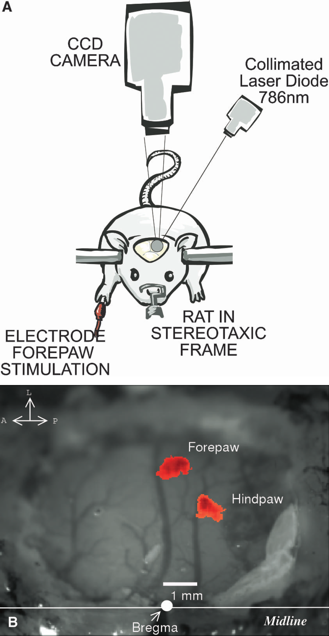
Figure 1A shows a sketch of the experimental set-up. A collimated, laser diode (Hitachi, HL 785 1G, 785nm, 50mW, Thorlabs, Newton, NJ, U.S.A.) driven by a custom-made driver illuminated the exposed cortex (approximately 5-mm diameter) at approximately 30 to 40 degrees from vertical. The laser beam was adjusted to provide uniform illumination of the surface of the brain tissue. Images were recorded by a 12-Bit, TEC cooled CCD camera (QImaging, Retiga 1350EX, Burnaby, B. C., Canada) using imaging software (StreamPix, NorPix, Montreal, Quebec, Canada). A 60-mm lens (AF Micro-Nikkor 60mm f/2.8D, Nikon, Melville, NY, U.S.A.) was used to focus the image and the aperture was adjusted so the speckle size matched the pixel dimensions (6.45 ° 6.45 μm) (Dunn et al., 2001). The camera was externally triggered at 5 Hz using the digital output of an A/D board (DataWave Technologies, Boulder, CO, U.S.A.). The A/D board was programmed to trigger the camera continuously (for 20 seconds); after the first 4 seconds it also triggered the stimulator with an identical signal for the chosen duration (i.e., for 4 or 8 seconds), thereby coregistering in time the data acquisition and stimulation. There was a 5-second interval between repeated stimulations where data were not acquired. The camera streamed output frames continuously through an IEEE 1394 port to the computer and a fast RAID array was used to store the frames. This prevented frame drops and allowed acquisition of approximately 1,000 × 1,000 pixel images at a rate up to 10 Hz, and smaller ROIs at even higher frame rates. This produced approximately 24 Gb of data per animal.

Fig. 1.

(A) A sketch of the laser-speckle imaging setup. The CCD camera is positioned over the exposed area with a slightly larger field of view than the craniectomy site. A collimated beam from a 785-nm laser diode illuminates the exposed brain tissue. (B) White-light image of the craniectomy at the contralateral side showing the location of bregma with the AFC response from the forepaw and hindpaw stimulation superimposed. The forepaw centroid is approximately 4 mm lateral to the bregma and is separated 1.8 mm from the hindpaw centroid.

Data analysis

Theory of laser-speckle flowmetry.

The theory underlying laser-speckle flowmetry has been described in detail (Briers, 2000, 2001). Laser speckle is a random interference pattern that arises when coherent laser light is scattered from a diffuse medium such as tissue. If the scattering particles in the medium are in motion (e.g., Brownian motion or flowing blood), then the speckle pattern fluctuates randomly. These intensity variations contain information about the velocity distribution of the scatterers. In laser-speckle flowmetry, blurring of the speckle pattern during the exposure time of a single image is used to extract blood-flow information. The depth sensitivity depends on the optical wavelengths used and may extend up to 1 mm, albeit with decreasing information at larger depths. The spatial resolution of the method is dependent on the speckle and camera pixel size, on the tissue surface, and on tissue scattering in the deeper tissues.

A window function of 5 × 5 (32.25 × 32.25-μm area) was scanned across the raw data, and the ratio of the standard deviation (σ) to the mean intensity (> I <) was calculated in each window. This quantity is referred to hereafter as speckle contrast, C(i,j), where i,j denote the pixel position. Images of C(i,j) show clear maps of the vasculature. To reduce the data to be processed to a manageable 2 Gb per animal, the images were smoothed using a bi-cubic intrapolation method by 5 × 5, thus reducing our spatial resolution to 32.25 μm.

The relative mean velocity of moving particles (i.e., the relative CBF) was extracted using the following relation (Briers, 2000; Bonner and Nossal, 1990):

C (i, j) = \frac{σ}{< I >} = {(\frac{τ_{c}}{2 T} (1 - e^{\frac{- 2 T}{τ_{c}}}))}^{2}

(1)

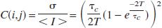
where τ_c = 1/(a k_ov) is the correlation time and T is the camera exposure time. Here, a is an unknown factor related to the Lorentzian width of the scattered spectrum and the scattering properties of the medium, v is a mean velocity, and k_o is the input light wavenumber. The mean velocity (v) was assumed to be proportional to CBF, and relative changes in flow (ΔCBF) were obtained by dividing each image by the baseline image. Twenty repeat stimulations were collapsed to one representative stimulation by aligning time points and calculating the mean and standard deviation of the images.

Correlation coefficient imaging.

The speckle images suffer from substantial physiologic and instrumental noise. A simple difference/ratio method neglects useful a priori information about the stimulus presentation. Therefore, we computed “correlation coefficient images” by calculating the correlation coefficient for each pixel (cc_i) with a simple step function describing the stimulus presentation [r_i (i = 1⋖N)] (Bandettini et al., 1993). The correlation coefficient is defined as

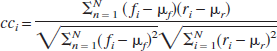
c c_{i} = \frac{Σ_{n = 1}^{N} (f_{i} - μ_{f}) (r_{i} - μ_{r})}{\sqrt{Σ_{n = 1}^{N} (f_{i} - μ_{f})^{2}} \sqrt{Σ_{n = 1}^{N} (f_{i} - μ_{f})^{2}}}

(2)

where f_i(i = 1 ⋖N) is the time course of ΔCBF for a given pixel, μ_f and μ_r are the mean values of f and r, and N is the number of frames. This was applied to all pixels in an averaged series, producing a single image representing the activation area. These images, rescaled (now cc'_i) by proportionally stretching the range to extend from 0 to 1, were used to calculate the centroid of the activation and to pick an ROI for the analysis of temporal and spatial response.

Temporal and spatial response.

The temporal response was reduced to a curve by defining an arbitrary but consistent ROI of all pixels with cc'_i > 0.95, which are averaged at each time point per series per animal. A low-pass filter was applied to reduce physiologic noise including the cardiac rhythm at approximately 5 Hz, and an average across animals was calculated. Larger ROIs were also examined and the qualitative shape of the response did not change with the choice of ROI.

To investigate the spatiotemporal response simultaneously, other ROIs were defined by either thresholding at varying ΔCBF levels, or as a function of distance from the activation centroid. The number of pixels within a given ROI at each time point was used to calculate an “area of activation.”

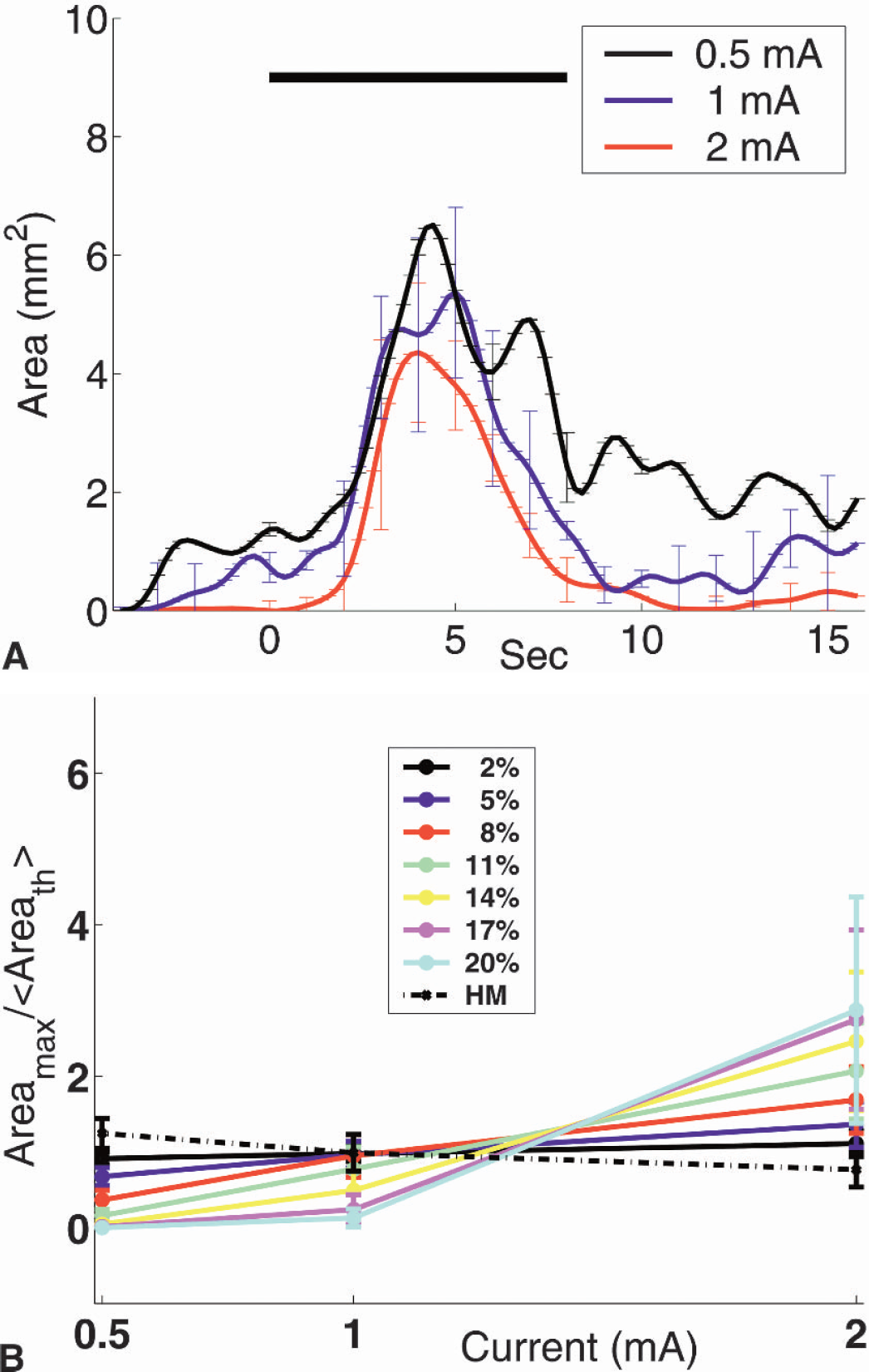
The area of activation was first defined by the number of pixels with ΔCBF above the half-maximum (threshold at half-height) response. To investigate the effect of the choice of threshold on this result, the threshold ΔCBF was varied from 2% to 20% in 3% increments. To quantify this response, the curves were averaged over 1 second around the peak (Area_max), and then normalized by the total mean over the three stimulation currents (0.5, 1, and 2 mA) (Area_th>) plotting $\frac{A r e a_{max}}{< A r e a_{t h} >}$ versus the stimulus current.

This normalization brought out the salient features by keeping the same scale for different thresholds. The time to reach maximum-area was defined to be the time to reach the peak in these plots.

Statistical analysis

Data were tested for statistical significance (when applicable) with repeated-measures analysis of variance. P>0.05 was used as the significance threshold. When the linearity of the dependence on stimulus amplitude was being tested, a Pearson correlation coefficient was further calculated and the corresponding R² and P value is reported with P>0.05 as the significance threshold.

RESULTS

Figure 1B shows a white-light photo of the craniectomy site with the location of bregma indicated and the AFC responses from a forepaw and a hindpaw stimulation superimposed. The forepaw centroid is approximately 4 mm lateral to bregma and is separated 1.8 mm from the hindpaw centroid. A similar result was obtained in the other rat where the two centroids were separated by 1.6 mm. Thus, the functional areas corresponding to forepaw and hindpaw areas are mapped as discrete, anatomically separate regions.

Figure 2 exhibits a sequence of images (200 ms/frame) showing the spatiotemporal evolution of the AFC response to an 8-second, 2-mA stimulation of the forepaw. The ROI, defined by ΔCBF > 7%, has been overlaid on the speckle contrast images. The stimulation was presented between the second 0 (ON) and 8 (OFF). The response reached a maximum after approximately 4 seconds and was followed by a relatively rapid decrease that was sustained for approximately 1 second after the stimulus was turned off.

Fig. 2.

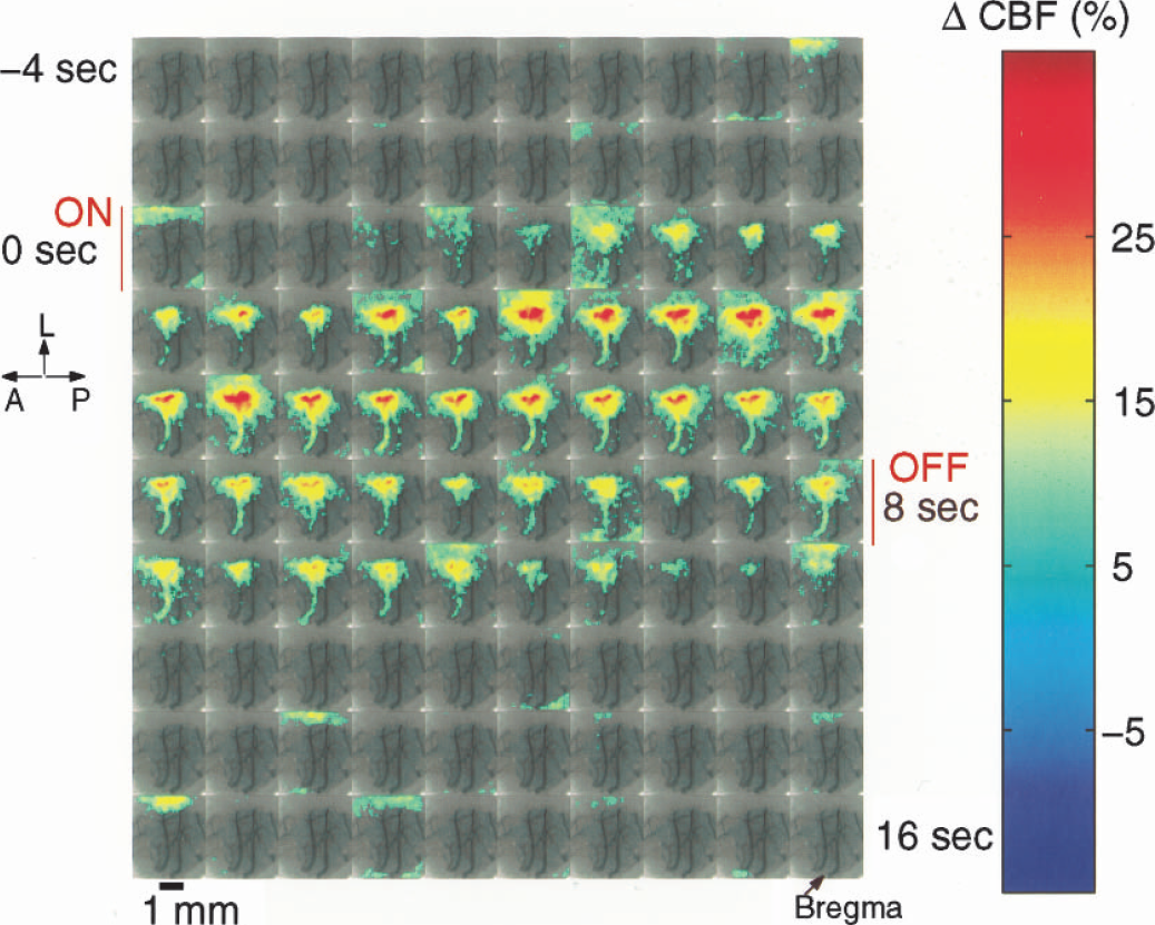
Time-series (200 ms/frame) of images showing the spatio-temporal evolution of the AFC response to 8-second, 2-mA stimulation of the forepaw. The ROI defined by ΔCBF > 7% is overlaid on the speckle contrast image. The stimulation is presented between seconds 0 (ON) and 8 (OFF). L, lateral; A, anterior, P, posterior.

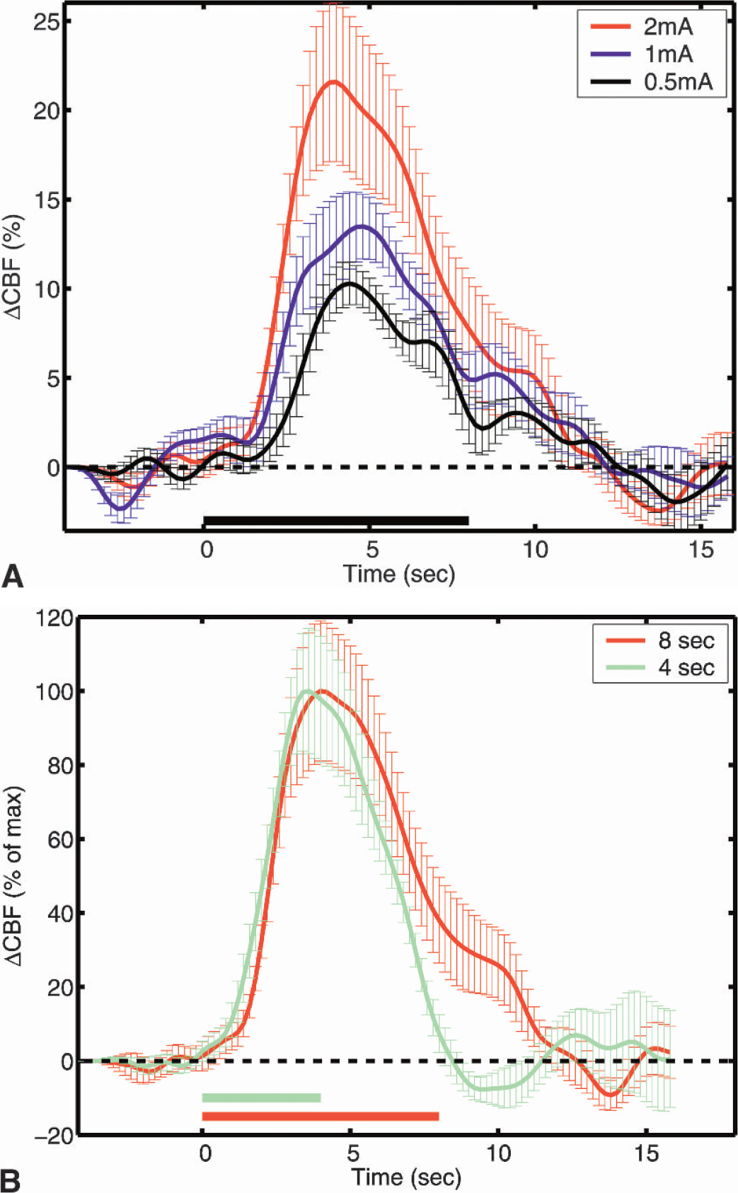
Figure 3 shows an image of cc'_i for a 2-mA, 8-second stimulation. Regions of interest for which cc'_i > 0.95 were defined to obtain integrated temporal response curves corresponding to the blood response to activation. Examination of the amplitude of the response to stimulation revealed a nearly linear peak response as a function of stimulus amplitude for the 8-second stimulus duration (Fig. 4A and Table 1). Similar results were obtained for the 4-second stimulus duration. Normalized responses (Fig. 4B) from the two stimulus durations (4 and 8 seconds) were the same for the first 4 seconds of the temporal trace. Blood flow decayed rapidly after reaching the peak and returned to the baseline after the end of the 4-second stimulus. The 8-second stimulus showed a delay of approximately 1 second decaying at a similar rate as the shorter stimulus curve until the end of the stimulus. After that point, the decay rate slowed down by a factor of four for approximately 2 seconds, which was followed by a more rapid decay over the next 2 seconds, reaching the baseline 4 seconds after the end of stimulus. This was independent of the stimulus amplitude.

Fig. 3.

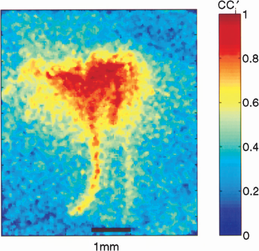
An image of cc'_i for a 2-mA, 8-second stimulation in one animal. The correlation coefficient (cc_i) between an input step function and the temporal evolution of the i^th pixel was calculated and rescaled to obtain cc'_i.

Fig. 4.

(A) ΔCBF in response to 8 seconds of stimulation at three different amplitudes—0.5 mA (black), 1 mA (blue), and 2 mA (red)—averaged over pixels with > 0.95 of maximal correlation coefficient. The peak response is nearly linear with stimulus amplitude. (B) Temporal characteristics of ΔCBF in response to two different stimuli durations (4 seconds [green] and 8 seconds [red]) at 2 mA averaged over pixels with > 0.95 of maximal correlation coefficient. Color coded horizontal bars indicate the stimulus presentation. Both curves are normalized by their peak value to bring out salient features related to the stimulus duration.

Table 1.

Time to peak and peak amplitude of ΔCBF as a function of stimulation duration and current

Duration(s)	Current(mA)	Time to peak*(s)	Peak*(%)
4	0.5	4.0 ± 1.2	10.2 ± 2.0
4	1	3.5 ± 1.2	13.4 ± 2.5
4	2	3.2 ± 1.5	20.0 ± 3.0
8	0.5	4.1 ± 1.3	10.2 ± 1.5
8	1	4.8 ± 1.1	13.2 ± 2.0
8	2	4.0 ± 1.2	21.4 ± 4.5

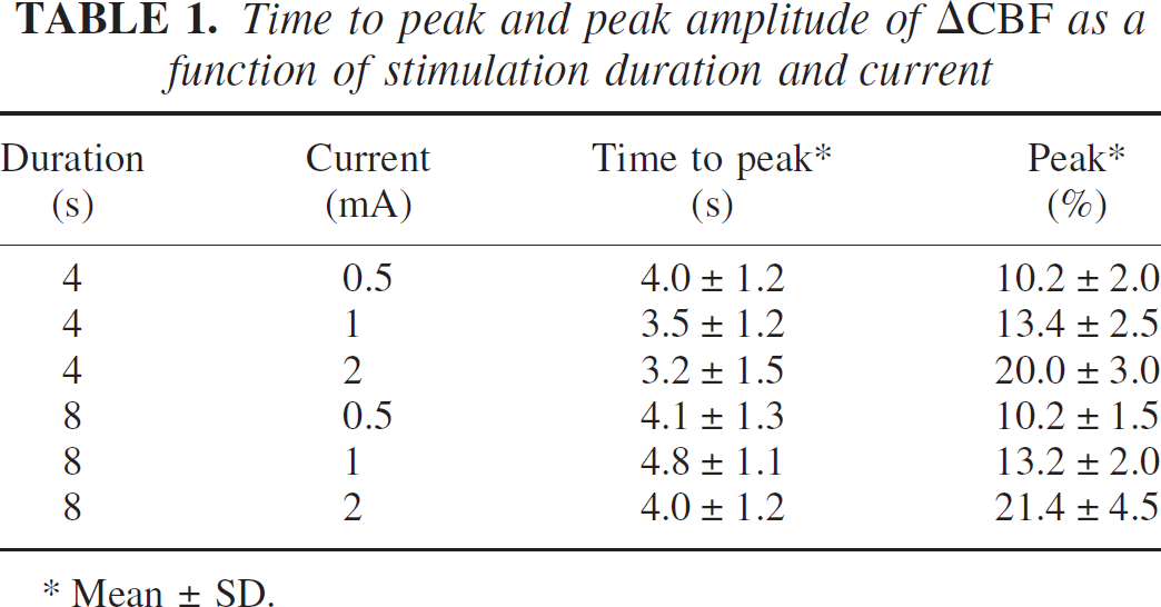
Mean ± SD.

Table 1 summarizes our findings in a parameterized manner for each stimulus condition. Time to peak was independent of stimulus duration and current (P > 0.2). Peak flow was linearly dependent on stimulus current (R² = 0.999, P>0.005 for 4 seconds, R² = 0.994, P>0.05 for 8 seconds).

The area of activation was defined by the number of pixels with ΔCBF above the half-maximum (threshold at half-height) response. Data for the 0.5-mA stimulus included a good deal of noise because the threshold was close to the noise floor of the frames, but there was no qualitative difference (P > 0.2) in the shape of the temporal evolution of the activation area with respect to stimulus amplitude (Fig. 5A). This effect, however, was threshold dependent. Low thresholds produced a larger activation area independent of stimulus amplitude, whereas high thresholds produced a smaller activation area with a dependence on stimulus amplitude (P>0.05). To quantify the response, the curves were averaged over 1 second around the peak, and then normalized by the total mean over the three stimulation currents (0.5, 1 and 2 mA). $\frac{A r e a_{max}}{< A r e a_{t h} >}$ versus stimulus current for different CBF thresholds are shown in Fig. 5B. This normalization brought out the salient features by keeping the same scale for different thresholds. For thresholds below 8%, the thresholded area of activation is independent of stimulation current (P = 0.5 [2%], P = 0.06 [5%]). The highest threshold (20%) measured mainly noise and was also independent of current (20%, P > 0.1). Table 2 summarizes the findings for half maximum threshold. The time to reach maximum-area was independent of stimulus current (P > 0.2).

Fig. 5.

(A) Area of activation obtained from the number of pixels with ΔCBF above the half-maximum response for three different stimuli amplitudes during 8-second stimulation. The stimulus period is shown by the black bar. There is no statistically significant difference in the activation area as a function of the stimulus amplitude. (B) Maximal area averaged over 1 second around the peak normalized by its mean over the three stimulation currents (0.5, 1, and 2 mA). The $\frac{A r e a_{max}}{< A r e a_{t h} >}$ versus current for different CBF thresholds. Half-maximum (HM) ΔCBF is shown by the dashed line. For thresholds below 8%, the thresholded area of activation is independent of stimulation current.

Table 2.

Activation area and time to reach maximal-area for different stimulus levels

Current(mA)	Maximal area*(mm²)	Time to maximal-area*(s)
0.5	6.5 ± 3.3	4.5 ± 1.4
1	5.4 ± 3.8	4.6 ± 0.9
2	4.4 ± 3.5	4.2 ± 0.7

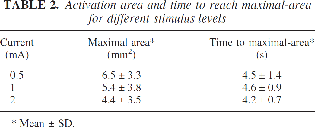
Mean ± SD.

Images of ΔCBF indicate regional dependence of the activation. To determine whether the shape of the temporal evolution of this response is constant with distance from the activation center, ROIs were defined as nonoverlapping, concentric rings of equal area around the activation centroid. The radius of the first filled ring was chosen to be approximately 0.5 mm. Twenty rings with increasing radii (maximum radius 2.29 mm) of equal area increments were used. The temporal response from every fourth ring is shown for simplicity in Fig. 6. Qualitative changes in temporal features of ring diameters were not observed, but the peak response decreases with increasing ring diameter.

Fig. 6.

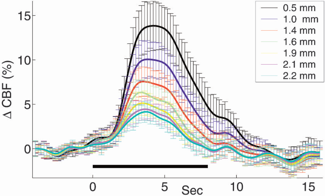
Equal area rings around the centroid of activation with radii indicated in the legend were chosen as regions of interest. The time course of ΔCBF(%) does not depend on the distance from the center of the activation. The solid bar represents the duration of stimulation.

DISCUSSION

The blood-flow response to electrical forepaw stimulation has been extensively characterized in our laboratory with laser-Doppler methods, identifying the stimulation frequency (5 Hz) for maximal response (Detre et al., 1998), showing a linear increase with amplitude (Detre et al., 1998), mapping the central location of maximal response (Ances et al., 1998, 1999), modeling the nonlinear effects (Ances et al., 2000), combining with changes in O₂ to estimate CMRO₂ (Ances et al., 2001a,c), and investigating the effect of carbon dioxide on the CBF response (Ances et al., 2001b).

Even though these studies have provided a great deal of information about the AFC response to forepaw stimulation, they were limited in various aspects because laser Doppler is essentially a point measurement. The other available alternative, scanning laser-Doppler imaging, offers high spatial resolution with a trade-off in temporal resolution, which limits its applicability in studies of the AFC (Ances et al., 1999). A high spatioresolution imaging technique that is relatively simple and inexpensive to implement is clearly desirable.

These results show that laser-speckle flowmetry is able to effectively measure, map. and characterize the CBF response to forepaw/hindpaw stimulation with high temporal and spatial resolution. The statistical methods used, including signal averaging and correlation coefficient imaging, improved the method's signal-to-noise ratio. This relatively simple technique, requiring only a laser diode, a CCD camera, and a computer, has provided new insights into previously relatively inaccessible aspects of the AFC.

A notable feature common to most images of relative blood flow is the presence of a large vessel above the threshold. This vessel appears to be a draining vein based on its width and proximity to the brain surface. This feature may hinder the identification of the activation area in relation to the neural representation but also delivers potentially useful physiologic information. A ROI chosen on the large vessel away from the central activation yielded a time course very similar to that in the parenchyma. It is possible to resolve vessels with diameter approximately 32 μm with the present system/analysis method.

Measurements of the temporal behavior of AFC at the center of activation yielded results that qualitatively agree with our previous data from laser-Doppler studies. However, the peak blood-flow response measured with speckle-contrast imaging is approximately 30% lower than that measured previously with laser-Doppler flowmetry (Detre et al., 1998). The physical and theoretical equivalence of the two techniques has been discussed at length by Briers (1996, 2001). Recently, Dunn and colleagues have found a high correlation between the two techniques under conditions of spreading depression and ischemia (Dunn et al., 2001). This high correlation may be attributed to the laminar homogeneity of the vascular response to both of these perturbations. Other studies, however, have shown some discrepancies between laser-Doppler flowmetry and laser-speckle flowmetry. Kharlamov and colleagues (2003) reported an underestimation of up to 35% by laser-speckle flowmetry in comparison with laser Doppler during hypercapnia. In a comparison study between the two techniques for measuring blood velocity in the optic nerve head, Yaoeda et al. (2000) also found a poor correlation.

We believe the differences seen in our forepaw activation studies may be due to factors including variations in animal preparation (open vs. closed skull) and differing depth sensitivity. During functional activation, the AFC response may not extend to the topmost layers, with the maximal response occurring at layers III through IV (approximately 600 μm below the cortical surface) (Chapin and Lin, 1984; Coq and Xerri, 1998; Duong et al., 2000). Laser-Doppler flowmetry, with near-infrared source wavelengths, was shown to be highly sensitive to layer IV, but had lower sensitivity to shallower levels (Fabricius et al., 1997). The depth sensitivity of laser speckle flowmetry begins immediately below the observed speckle and degrades rapidly from the surface. This has been modeled by Monte-Carlo methods revealing that most of the information comes from the top approximately 300 μm of the cortical tissue when the illuminating wavelength is 785 nm Kohl et al. (2000). Although both techniques probe to similar depths, their partial volume effects are different. As the laser-speckle flowmetry is further tested in the brain, a better understanding of these differences should emerge.

The amplitude of the response was found to monotonically increase with increasing stimulus current in a linear fashion. As expected, the longer stimulus duration (8 seconds) led to a CBF response that had behaved in a somewhat complex manner, suggestive of a peak-plateau time course (Ances et al., 2000). The activation decayed in amplitude with distance from the centroid. By examining ROIs surrounding the central peak, it was observed that the AFC response behaves temporally similarly in all regions activated by the forepaw stimulation. It has a spatially decaying profile across the field of view, but with the same temporal properties.

The AFC response was well localized and different functional representations of the forepaw and hindpaw were separated by 1.6 to 8 mm, in close agreement with previous results from electrophysiology wherein the areas were determined to be approximately 1.8 mm apart (Chapin and Lin, 1984).

Another characteristic of the response that has not been possible to measure with point laser-Doppler probes is the dependence of activation area on stimulus parameters. It was found that stimulus area does not change with either the stimulus amplitude or duration. As expected, this result is threshold dependent. Half-height values provide a normalized threshold; the area of activation at this threshold level was independent of the stimulus amplitude. However, measurements above an approximately 8% threshold showed that the activation area depended on stimulus amplitude. This is a common issue in imaging modalities and extra care should be taken when comparing results from different experiments. The attempt at normalization by using the half-height of the flow response as the threshold level as well as statistical approaches can provide a way to cross-validate results between different modalities.

The AFC area at half-height evaluated by laser-speckle flowmetry was between 4.4 ± 3.5 mm² and 6.5 ± 3.3 mm². Assuming that our stimulus extends to several digits, this area is similar to electrophysical measurements, which found that the cortical area activated was about 1.5 mm² per digit stimulated (Chapin and Lin, 1984; Coq and Xerri, 1998). It is also qualitatively similar to other hemodynamic measurements, such as those of diffuse optical tomography (Culver et al., 2003b), functional magnetic resonance imaging (Duong et al., 2000; Hyder et al., 1994; Mandeville et al., 1998), and optical intrinsic signal imaging (Narayan et al., 1994).

CONCLUSION

Laser-speckle flowmetry was used for the first time to characterize activation flow coupling after somatosensory stimulation. This technique provides high spatiotemporal information and is ideal for the study of basic functional mapping as well as for characterizing the AFC response. It can easily be combined with other optical techniques including optical intrinsic imaging (Dunn et al., 2003), diffuse optical tomography (Culver et al., 2003b; Yu et al., 2003), and diffuse correlation tomography (Culver et al., 2003a) for simultaneous measurement of tissue oxygen saturation, total hemoglobin concentration, and oxygen consumption, and for low-resolution three-dimensional imaging. Future studies of fundamental brain pathophysiology in animal models and in human subjects are feasible.

Footnotes

Acknowledgments:

The authors thank B. Ances, A. Dunn, J. P. Culver, and R. Choe for their helpful comments.

References

Ances

Buerk

Greenberg

Detre

(2001a) Temporal dynamics of the partial pressure of brain tissue oxygen during functional forepaw stimulation in rats. Neurosci Lett 306:106–110

Ances

Detre

Takahashi

Greenberg

(1998) Transcranial laser Doppler mapping of activation flow coupling of the rat somatosensory cortex. Neurosci Lett 257:25–28

Ances

Greenberg

Detre

(1999) Laser doppler imaging of activation-flow coupling in the rat somatosensory cortex. Neuroimage 10:716–723

Ances

Greenberg

Detre

(2001b) The effects of graded hypercapnia on the activation flow coupling response due to forepaw stimulation in =-chloralose anesthetized rats. Brain Res 911:82–88

Ances

Wilson

Greenberg

Detre

(2001c) Dynamic changes in cerebral blood flow, O-2 tension, and calculated cerebral metabolic rate of O-2 during functional activation using oxygen phosphorescence quenching. J Cereb Blood Flow Metab 21:511–516

Ances

Zarahn

Greenberg

Detre

(2000) Coupling of neural activation to blood flow in the somatosensory cortex of rats is time-intensity separable, but not linear. J Cereb Blood Flow Metab 20:921–930

Bandettini

Jesmanowicz

Wong

Hyde

(1993) Processing strategies for time-course data sets in functional MRI of the human brain. Mag Res Med 30:161–173

Boas

Yodh

(1997) Spatially varying dynamical properties of turbid media probed with diffusing temporal light correlation. J Opt Soc Am A 14:192–215

Bolay

Reuter

Dunn

Huang

Boas

Moskowitz

(2002) Intrinsic brain activity triggers trigeminal meningeal afferents in a migraine model. Nat Med 8:136–142

10.

Bonner

Nossal

(1990) Principles of laser-Doppler flowmetry. In: Laser-Doppler blood flowmetry, Vol 107. Shepard Alber

and Öberg

P Ake

, editors. Boston: Kluwer Academic Publishers, pp. 17–45

11.

Briers

(1996) Laser Doppler and time-varying speckle: a reconciliation. J Opt Soc Am A 13:345–350

12.

Briers

(2000) Time-varying speckle for measuring motion and flow. In: Saratov fall meeting 2000 report, Saratov, Russia

13.

Briers

(2001) Laser doppler, speckle and related techniques for blood perfusion mapping and imaging. Physiol Meas 22:R35–R66

14.

Briers

Webster

(1996) Laser speckle contrast analysis (LASCA): a nonscanning, full-field technique for monitoring capillary blood flow. J Biomed Opt 1:174–179

15.

Chapin

Lin

(1984) Mapping the body representation in the SI cortex of anesthetized and awake rats. J Comp Neurol 229:199–213

16.

Cheung

Culver

Takahashi

Greenberg

Yodh

(2001) In vivo cerebrovascular measurement combining diffuse near-infrared absorption and correlation spectroscopies. Phys Med Biol 46:2053–2065

17.

Coq

Xerri

(1998) Environmental enrichment alters organizational features of the forepaw representation in the primary somatosensory cortex of adult rats. Exp Brain Res 121:191–204

18.

Culver

Durduran

Furuya

Cheung

Greenberg

Yodh

(2003a) Diffuse optical tomography of cerebral blood flow, oxygenation and metabolism in rat during focal ischemia. J Cereb Blood Flow Metab 23:911–924

19.

Culver

Siegel

Stott

Boas

(2003b) Volumetric diffuse optical tomography of brain activity. Opt Lett 28:2061–2063

20.

Detre

Ances

Takahashi

Greenberg

(1998) Signal averaged laser doppler measurements of activation-flow coupling in the rat forepaw somatosensory cortex. Brain Res 796:91–98

21.

Dunn

Bolay

Moskowitz

Boas

(2001) Dynamic imaging of cerebral blood flow using laser speckle. J Cereb Blood Flow Metab 21:195–201

22.

Dunn

Devor

Bolay

Andermann

Moskowitz

Dale

Boas

(2003) Simultaneous imaging of total cerebral hemoglobin concentration, oxygenation, and blood flow during functional activation. Opt Lett 28:28–30

23.

Duong

Silva

Lee

Kim

(2000) Functional MRI of calcium-dependent synaptic activity: cross correlation with CBF and BOLD measurements. Mag Res Med 43:383–392

24.

Fabricius

Akgoren

Dirnagl

Lauritzen

(1997) Laminar analysis of cerebral blood flow in cortex of rats by laser-Doppler flowmetry: a pilot study. J Cereb Blood Flow Metab 17:1326–1336

25.

Frackowiak

Lenzi

Jones

Heather

(1980) Quantitative measurement of regional cerebral blood flow and oxygen metabolism in man using 150 and positron emission tomography: theory, procedure, and normal values. J Comput Assist Tomogr 4:727–736

26.

Fujii

Asakura

Nohira

Shintomi

Ohura

(1985) Blood flow observed by time-varying laser speckle. Opt Lett 10:104–106

27.

Hyder

Behar

Martin

Blamire

Shulman

(1994) Dynamic magnetic resonance imaging of the rat brain during forepaw stimulation. J Cereb Blood Flow Metab 14:649–655

28.

Kharlamov

Brown

Easley

Jones

(2003) Heterogeneous changes in cerebral blood flow during hypotension demonstrated by laser speckle technique. J Cereb Blood Flow Metab Suppl 23(S1):84

29.

Kim

(1995) Quantification of relative cerebral blood flow change by flow-sensitive alternating inversion recovery (FAIR) technique: application to functional mapping. Mag Res Med 34:293–301

30.

Kohl

Lindauer

Royl

Kuhl

Gold

Villringer

Dirnagl

(2000) Physical model for the spectroscopic analysis of cortical intrinsic optical signals. Phys Med Biol 45:3749–3764

31.

Kwong

Belliveau

Chesler

Goldberg

Weisskoff

Poncelet

Kennedy

Hoppel

Cohen

Turner

Cheng

Brady

Rosen

(1992) Dynamic magnetic resonance imaging of human brain activity during primary sensory stimulation. Proc. Natl Acad Sci U S A 89:5675–5679

32.

Lou

Edvinsson

Mackenzie

(1987) The concept of coupling blood-flow to brain-function - revision required. Ann Neurol 22:289–297

33.

Mandeville

Marota

Kosofsky

Keltner

Weissleder

Rosen

Weisskoff

(1998) Dynamic functional imaging of relative cerebral blood volume during rat forepaw stimulation. Mag Res Med 39:615–624

34.

Narayan

Santori

Blood

Burton

Toga

(1994) Imaging optical reflectance in rodent barrel and forelimb sensory cortex. Neuroimage 1:181–190

35.

Nielsen

Fabricius

Lauritzen

(2000) Scanning laser-doppler flowmetry of rat cerebral circulation during cortical spreading depression. J Vasc Res 37:513–522

36.

Ruth

(1994) Measuring the steady-state value and the dynamics of the skin blood flow using the non-contact laser speckle method. Med Eng Phys 16:105–111

37.

Sakurada

Kennedy

Jehle

Brown

Carbin

Sokoloff

(1978) Measurement of local cerebral blood flow with iodo (14c) antipyrine. Am J Physiol 234:H59–H66

38.

Tamaki

Araie

Kawamoto

Eguchi

Fujii

(1994) Non-contact two-dimensional measurement of retinal microcirculation using laser speckle phenomenon. Invest Ophthalmol Vis Sci 35:3825–3834

39.

Van Heertum

Tikofsky

(2000) Functional cerebral SPECT in PET imaging. Philadelphia: Lippincott Williams & Wilkins

40.

Villringer

Dirnagl

(1995) Coupling of brain activity and cerebral blood flow: basis of functional neuroimaging. Cereb Brain Metab Rev 7:240–276

41.

Yaoeda

Shirakashi

Funaki

Nakatsue

Abe

(2000) Measurement of microcirculation in the optic nerve head by laser speckle flowgraphy and scanning laser Doppler flowmetry. Am J Ophthalmol 129:734–739

42.

Durduran

Furuya

Greenberg

Yodh

(2003) Frequency-domain multiplexing system for in vivo diffuse light measurements of rapid cerebral hemodynamics. Appl Opt 42:2931–2939

Spatiotemporal Quantification of Cerebral Blood Flow during Functional Activation in Rat Somatosensory Cortex using Laser-Speckle Flowmetry

Abstract

Keywords

MATERIALS AND METHODS

Surgical preparation and stimulus presentation

Laser-speckle flowmetry instrument

Data analysis

Theory of laser-speckle flowmetry.

Correlation coefficient imaging.

Temporal and spatial response.

Statistical analysis

RESULTS

DISCUSSION

CONCLUSION

Footnotes

Acknowledgments:

References