Sage Journals: Discover world-class research

Abstract

Changes in cerebral blood flow (CBF) because of functional activation are used as a surrogate for neural activity in many functional neuroimaging studies. In these studies, it is often assumed that the CBF response is a linear-time invariant (LTI) transform of the underlying neural activity. By using a previously developed animal model system of electrical forepaw stimulation in rats (n = 11), laser Doppler measurements of CBF, and somatosensory evoked potentials, measurements of neural activity were obtained when the stimulus duration and intensity were separately varied. These two sets of time series data were used to assess the LTI assumption. The CBF data were modeled as a transform of neural activity (N₁–P₂ amplitude of the somatosensory evoked potential) by using first-order (linear) and second-order (nonlinear) components. Although a pure LTI model explained a large amount of the variance in the data for changes in stimulus duration, our results demonstrated that the second-order kernel (i.e., a nonlinear component) contributed an explanatory component that is both statistically significant and appreciable in magnitude. For variations in stimulus intensity, a pure LTI model explained almost all of the variance in the CBF data. In particular, the shape of the CBF response did not depend on intensity of neural activity when duration was held constant (time-intensity separability). These results have important implications for the analysis and interpretation of neuroimaging data.

Keywords

Linear-time invariant transform Activation-flow coupling Cerebral blood flow Time-intensity separability

In many neuroimaging techniques, changes in cerebral blood flow (CBF) or related hemodynamic measures are used as a surrogate marker for changes in neural activity (Bandettini et al., 1992; Ogawa et al., 1990, 1992). This relationship between neural activity and CBF is known as activation-flow coupling (AFC) (Ances et al., 1998; Detre et al., 1998). However, a full description of the AFC transformation is not known. The assumed nature of the AFC transform will impact the validity of inferences that predict neural activity changes based on observed hemodynamic measures (Friston et al., 1995a, b , c ; Josephs and Henson, 1999; Vazquez and Noll, 1998).

A linear-time invariant (LTI) system is one that transforms input to output via convolution with an impulse-response function, the response of the system to an input of vanishingly brief duration (Oppenheim et al., 1983). In the context of the AFC system, the input is neural activity and the output is the CBF response. LTI systems obey scaling and superposition, and so they allow quite straightforward inference about inputs based on outputs. Therefore, it is not surprising that the many neuroimaging analyses assume, either explicitly or implicitly, that the AFC system is LTI (Boynton et al., 1996; Dale and Buckner, 1997).

In theory, it is elementary to test for an LTI transformation by using suitable statistical methods to determine if there exists an impulse-response function that can predict the output signal from the input signal via convolution. In the context of the AFC system used for neuroimaging, there exists a practical difficulty in testing for LTI, because it is not trivial to obtain localized estimates of both neural activity and CBF. As a consequence, in all neuroimaging studies to date, which have tested for an LTI in the AFC system of humans, the CBF response has been measured and neural activity has been assumed to be bear a simple relationship to experimental parameters such as stimulus duration and intensity (Boynton et al., 1996; Dale and Buckner, 1997; Josephs and Henson, 1999; Rees et al., 1997; Vazquez and Noll, 1998).

Authors of two studies that used animal models have examined the relationship between neural activity and the CBF response more directly by measuring both evoked electrical potentials and CBF changes (Mathiesen et al., 1998, 2000; Ngai et al., 1999). Both of these studies demonstrated a positive correlation between changes in CBF and measurements of neural activity, as would be predicted by an LTI model. We have extended this analysis in the current study. By using a previously validated rat model system (Ances et al., 1998; Detre et al., 1998), we measured local changes in CBF by using laser Doppler (LD) and local neural activity, as measured by somatosensory evoked potentials (SSEPs), as a result of electrical forepaw stimulation. Two parameters of the sensory stimulation, duration and intensity, were varied to alter the form of the associated neural response. The relationship between the measured neural and CBF responses was modeled with linear and nonlinear components (Bendat, 1990; Friston et al., 1998). Under an LTI transform, there would be no explanatory contribution from the nonlinear components.

MATERIALS AND METHODS

Surgical preparation

Adult male Sprague-Dawley rats (300 to 380 g; n = 11) obtained from Charles River (Wilmington, MA, U.S.A) were initially anesthetized with 1% to 2% halothane in 70% N₂0:30% O₂ by use of a facemask. The tail artery was cannulated with a polyethylene catheter (PE-50; Clay Adams, Becton Dickinson Primary Care Diagnostics, Sparks, MO, U.S.A.) for measurement of arterial blood pressure and arterial blood gases. The rats were tracheotomized, mechanically ventilated, and maintained on 1% halothane in 70% N₂0:30% O₂. The head was then secured into a stereotaxic frame and a midline scalp incision made with the scalp retracted over the frontoparietal cortex. A 3 × 3-mm-wide square area overlying the forepaw portion of the somatosensory cortex was thinned by using a saline-cooled dental drill (Star Titan Low Speed Dental Drill; Star Dental, Lancaster, PA, U.S.A.) until only a thin translucent cranial plate remained. Halothane was discontinued after surgery and for at least 45 minutes before data acquisition. After surgery and during all stimulation studies, anesthesia was maintained with 60 mg/kg of α-chloralose given intraperitoneally, followed by hourly supplemental intraperitoneal doses of 30 mg/kg (Bonvento et al., 1994). A tail pinch was administered before each supplemental dose of α-chloralose to ensure adequate depth of anesthesia. Body temperature was monitored with a rectal probe and maintained at 37.0°C ± 0.5°C by using a heating pad. An arterial blood pressure tracing was obtained at all times to ensure that changes in local CBF were not the result of systemic blood pressure changes (Detre et al., 1998). Arterial blood gases were measured approximately every 45 minutes. Ventilation parameters were adjusted to maintain the Paco₂ at 32 to 39 mm Hg.

Forepaw stimulation

Electrical forepaw stimulation was performed using two subdermal needle electrodes inserted into the dorsal forepaw. A function generator (Global Specialties, New Haven, CT, U.S.A) was used to control the stimulus frequency. This frequency was set at 5 Hz, and the pulse width was maintained at 1.0 milliseconds. This frequency was chosen because it has previously been demonstrated to lead to maximal changes in CBF (Detre et al., 1998). The stimulus intensity was controlled (Detre et al., 1998) using a constant current dense stimulus isolation device (A-36V; World Precision Instruments, San Diego, CA, U.S.A). A micromanipulator on a stereotactic co-ordinate system (Stoelting, Wood Dale, IL, U.S.A.) was used to ensure that the probe was normal to the thinned skull. The LD probe (Vasamedics, St. Paul, MN, U.S.A) was positioned 5 mm lateral to bregma (Ances et al., 1998) with all LD measurements recorded with a time constant of 0.5 second.

Experimental stimulation protocols

Study I

For some rats (n = 8), the stimulus duration was varied and the stimulus intensity was fixed at 1. 0 mA. The stimulus duration levels were 2, 4, 8, and 16 seconds. For all trials, for the different stimulus duration levels, a 4-second “baseline” period preceded the stimulus and a 16-second period succeeded stimulation. Thus, the four levels of the stimulus duration factor corresponded to trial lengths of 22, 24, 28, and 36 seconds.

Study II

For some rats (n = 8; with an overlap of 5 rats from the sample used in study I), the stimulus intensity was varied and the stimulus duration was fixed at 4 seconds. The different stimulus intensity levels were 0.5, 1, and 2 mA. For all trials, for the different stimulus intensity levels, a 4-second baseline period preceded the stimulus and a 16-second period succeeded stimulation. Thus, all three levels of the stimulus intensity factors had a trial length of 24 seconds.

Data analysis of CBF measurements by using LD

For both variations in the stimulus duration (study I) and stimulus intensity (study II), the LD signal was acquired at a sampling rate of 10 Hz. All LD data were saved as raw voltages and converted to percent changes from baseline by dividing the value observed by the average baseline flow for the 4 seconds before stimulus application.

A set of 10 trials was administered at each stimulus duration (study I) or stimulus intensity (study II). For each level of the relevant parameter, a minimum of two sets of trials was performed per rat. For study I, only the first trial of each set of 10 was retained for analysis. This decision (made after preliminary data analysis) was implemented to eliminate apparent CBF refractoriness effects associated with repetitive periodic stimulation. Thus, the CBF signals corresponding to a given stimulus duration in study I represent the average of two stimulus trials, which correspond to the first stimulus of each of the two sets of 10. Because the same stimulus duration and interstimulus interval was used in all trials of study II, the CBF signals that correspond to a given stimulus intensity were averaged across all 10 trials from both sets.

Somatosensory evoked potentials

SSEPs and LD measurements were recorded separately, with SSEP measurements interleaved with LD results. SSEPs were recorded with stainless steel screws inserted into the skull and secured with dental cement. One electrode was placed immediately behind the thinned skull and a reference electrode was placed frontally near the midline suture.

Evoked potentials were amplified by using a Grass Polygraph EEG amplifier (Model 7D; Grass Instruments, Boston, MA, U.S.A) with bandpass frequencies of 10 Hz to 3 kHz and were averaged using a Labview virtual instrument. Stimulus conditions were identical to those used for LD measurements, except that a stimulus frequency of 4.7 Hz was used, instead of 5 Hz, to avoid 60-Hz interference. Data were acquired at 20 kHz, starting 10 milliseconds before the forepaw stimulus, and continued for 60 milliseconds. The stimulus trigger was recorded in a separate channel, and a peak detection algorithm for this channel was used to temporally align data for signal averaging. A single set consisted of 200 evoked potentials with at least two sets performed for each of the stimulus durations and intensities for each rat.

The SSEP data preprocessing yielded a single SSEP waveform per level of the stimulus duration and intensity factor per rat. These were averaged across rats to yield a single SSEP waveform per stimulus duration and intensity. From each of these waveforms, the N₁–P₂ amplitude was determined and used as a measure of neuronal activity (Di and Barth, 1991; Dirnagl et al., 1993; Lindauer et al., 1996; Narayan et al., 1994; Ngai et al., 1999).

Determination of the amplitude of neural activity during the stimulus time periods

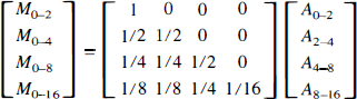
For study I, we were able to determine directly the average amplitudes of the SSEP response during the periods 0 to 2 seconds (e.g., amplitude M_0–2), 0 to 4 seconds (M_0–4), 0 to 8 seconds (M_0–8), and 0 to 16 seconds (M_0—16). The relationship between the average SSEP amplitude during the periods 0 to 2 seconds (A_0–2), 2 to 4 seconds (A_2–4), 4 to 8 seconds (A_4–8), and 8 to 16 seconds (A_8—16) after stimulation and [M_0–2, M_0–4, M_0–8, M_0–16] is given by the following linear system of equations:

[\begin{matrix} M_{0 - 2} \\ M_{0 - 4} \\ M_{0 - 8} \\ M_{0 - 16} \end{matrix}] = [\begin{matrix} 1 & 0 & 0 & 0 \\ 1 / 2 & 1 / 2 & 0 & 0 \\ 1 / 4 & 1 / 4 & 1 / 2 & 0 \\ 1 / 8 & 1 / 8 & 1 / 4 & 1 / 16 \end{matrix}] [\begin{matrix} A_{0 - 2} \\ A_{2 - 4} \\ A_{4 - 8} \\ A_{8 - 16} \end{matrix}]

(1)

which was solved for [A_0–2, A_2–4, A_4–8, A_8–16]^T. This allowed approximate neural input functions to be generated. Let n_i(mΔT) be the approximated neural input function corresponding to stimulus duration i (where m is an integer starting from 0, and ΔT is the sampling period of the LD data). We defined the n_i(mΔT) as follows:

\begin{aligned} n_{2 \sec} (m Δ T) = & A_{0 - 2} u (m Δ T) - A_{0 - 2} u (m Δ T - 2) \\ n_{4 \sec} (m Δ T) = & n_{2 \sec} (m Δ T) + A_{2 - 4} u (m Δ T - 2) \\ - A_{2 - 4} u (m Δ T - 4) \\ n_{8 \sec} (m Δ T) = & n_{4 \sec} (m Δ T) + A_{4 - 8} u (m Δ T - 4) \\ - A_{4 - 8} u (m Δ T - 8) \\ n_{16 \sec} (m Δ T) = & n_{8 \sec} (m Δ T) + A_{8 - 16} u (m Δ T - 8) \\ - A_{8 - 16} u (m Δ T - 16) \end{aligned}

(2)

where u(mΔT) is the Heaviside (or step) function, as follows: u(mΔT) = 1 for mΔT ≥ 0; u(mΔT) = 0 for mΔT < 0. For analysis purposes, the n_i(mΔT) values were concatenated in time to yield a single vector n(mΔT).

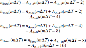
For study II, the generation of approximate neural activity amplitude time series for the different stimulus intensities was more elementary. Let A_I be the averaged SSEP amplitude associated with stimulus intensity I, and let n_i(mΔT) be the approximated neural activity time series corresponding to stimulus intensity i. We specified the n_i(mΔT) as follows:

n_{i} (m Δ T) = A_{i} u (m Δ T) - A_{i} u (m Δ T - 4)

(3)

Modeling of the AFC system

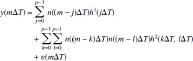
The AFC system mediates the transform of changes in neural activity to changes in CBF. This section describes how the AFC system was modeled. The LD time series corresponding to the different levels of stimulus duration (study I) or stimulus intensity (study II) were concatenated in time to yield a single vector y(mΔT) for each study. Each of these concatenated LD time series was fit with two models. Model 1 was a causal, finite response LTI model with output noise

y (m Δ T) = \sum_{j = 0}^{p - 1} n ((m - j) Δ T) h^{1} (j Δ T) + ε (m Δ T)

(4)

where n(mΔT) is the approximated neural input function (see preceding section), h¹(mΔT) is an unknown impulse response function, and ε(mΔT) is an independent and identically distributed error process. Based on previous information about the temporal dynamics of the CBF response (Ances et al., 1998; Detre et al., 1998; Dirnagl et al., 1994; Ngai and Winn, 1995), it was assumed in the current analysis that the duration of the IRF h¹(mΔT) would be ≤ 12 seconds. h¹(mΔT) was thus expanded, in terms of a set of sines and cosines (with periods of 12, 6, and 4 seconds), as follows:

\begin{aligned} h^{1} (m Δ T) = & (u (m Δ T) - u (m Δ T - p Δ T)) \\ [\sum_{b = 0}^{3} d_{b} \cos (2 π b m Δ T / 12) \\ + \sum_{b = 1}^{3} c_{b} \sin (2 π b m Δ T / 12)] \end{aligned}

(5)

where pΔT is the assumed duration of the finite system response (pΔT = 12 seconds in this case), and the c_b and d_b are unknown parameters. When Eq. 5 is substituted into Eq. 4, one obtains a general linear model (Friston et al., 1994, 1995a, b , c , 1998) that involves the unknown parameters c_b and d_b. One can estimate these parameters via ordinary least-squares (Friston et al., 1998). The purpose of applying model 1 was to see how validly a pure LTI transform could describe the relationship between the approximated neuronal input and CBF for the different stimulus durations and intensities.

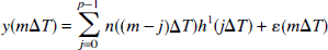
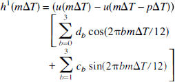
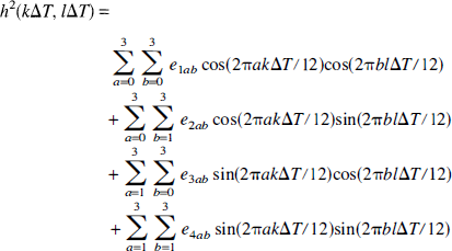
As follows, model 2 was a second-order Volterra series (Friston et al., 1998):

\begin{aligned} y (m Δ T) = & \sum_{j = 0}^{p - 1} n ((m - j) Δ T) h^{1} (j Δ T) \\ + \sum_{k = 0}^{p - 1} \sum_{l = 0}^{p - 1} n ((m - k) Δ T) n ((m - l) Δ T) h^{2} (k Δ T, l Δ T) \\ + ε (m Δ T) \end{aligned}

(6)

where h¹(mΔT) is the first-order Volterra kernel and h²(kΔT,lΔT) is the second-order Volterra kernel. We again assume Eq. 4 for h¹(mΔT). For h²(kΔT,lΔT), we assume the following expansion:

\begin{aligned} h^{2} (k Δ T, l Δ T) = \\ \sum_{a = 0}^{3} \sum_{b = 0}^{3} e_{1 a b} \cos (2 π a k Δ T / 12) \cos (2 π b l Δ T / 12) \\ \sum_{a = 0}^{3} \sum_{b = 1}^{3} e_{2 a b} \cos (2 π a k Δ T / 12) \sin (2 π b l Δ T / 12) \\ \sum_{a = 1}^{3} \sum_{b = 0}^{3} e_{3 a b} \sin (2 π a k Δ T / 12) \cos (2 π b l Δ T / 12) \\ \sum_{a = 1}^{3} \sum_{b = 1}^{3} e_{4 a b} \sin (2 π a k Δ T / 12) \cos (2 π b l Δ T / 12) \end{aligned}

(7)

which also yields a general linear model for Eq. 6 in the unknown parameters (estimated with ordinary least-squares) c_b and d_b (corresponding to the first-order kernel) and e_iab (corresponding to the second-order kernel; Friston et al., 1998). If the transform between neuronal activity and CBF were LTI, then the value of all of the second-order kernel parameters would be zero. Thus, the question of whether the system has a nonlinear component can be addressed statistically with an F-test for the net explanatory contribution of the partition of the parameters corresponding to the second-order kernel (Friston et al., 1998).

Standard statistical inference assumes independent errors (Johnston, 1972). However, examination of the power spectrum of the residuals of the ordinary least-squares fit of model 2 revealed a strong violation of this assumption. This is expected, given the 0.5-second time constant of LD data acquisition. Therefore, the LD time series y(mΔT) was smoothed with a Gaussian kernel (σ = 0.5 second). The effect of smoothing is to make statistical inference more robust to incorrect specification of the intrinsic autocorrelation structure. This smoothing was explicitly accounted for in the ensuing statistical inferences (Worsley and Friston, 1995).

RESULTS

Physiologic variables

Physiologic parameters for this study I (effect of variations in the stimulus duration) were as follows: MAP = 101 ± 4 mm Hg; pH = 7.38 ± 0.04; P_aCO₂ = 34.2 ± 2.7 mm Hg; and P_aCO₂ = 118 ± 5 mm Hg (mean ± SD; n = 8). Physiologic parameters for study II (effect of variations in the stimulus intensity) were as follows: MAP = 102 ± 3 mm Hg; pH = 7.38 ± 0.03; P_aCO₂ = 34.7 ± 2.1 mm Hg; and P_aCO₂ = 116 ± 4 mm Hg (mean ± SD; n = 8). There were no significant differences between the two study groups for the different parameters.

Study I

Qualitative effect of stimulus duration on the CBF response

A characteristic peak change in the CBF response was seen for shorter stimuli of 2 and 4 seconds in duration (Figs. 1A and 1B). For stimuli longer than 4 seconds (8 and 16 seconds stimuli), the shape of the CBF responses consisted of an initial peak response followed by a plateau phase that persisted for the length of the stimulus (Figs. 1C and 1D). There was no detectable effect of forepaw stimulation on the systemic blood pressure at any of the stimulus duration (insets for Figs. 1A through 1D). This result suggests that there was no global blood flow effect that contaminated the local LD signal.

FIG. 1.

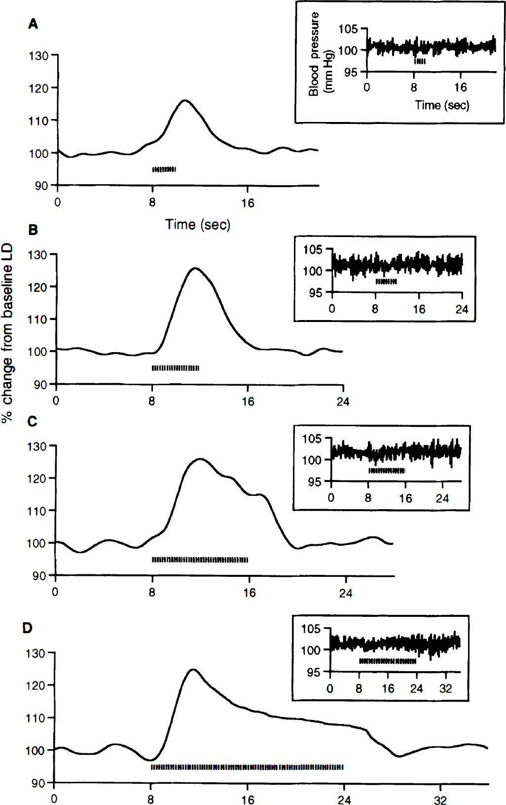
Cerebral blood flow (CBF) responses averaged over rats (n = 8) for different stimulus durations of 2 seconds (A), 4 seconds (B), 8 seconds (C), and 16 seconds (D) stimuli. Insets: Average blood pressure traces for 2 seconds (A), 4 seconds (B), 8 seconds (C), and 16 seconds (D) stimuli. For all stimuli ≤ 4 seconds a peak CBF response was observed while stimuli > 4 seconds led to a peak and plateau. Hashed lines indicate stimulus duration. No significant blood pressure changes were seen for the different stimulus durations.

SSEP measurements for different stimulus durations

Evoked potentials were reliably recorded from the same hemisphere in which CBF changes were measured by LD from all rats (n = 8). Figure 2 shows characteristic SSEP responses averaged from a minimum of two sets of 200 evoked potentials from a single representative rat for the different stimulus durations. The typical SSEP response for all stimuli consisted of an initial positive wave (P₁), then a negative (N₁) wave, followed by a second positive peak (P₂). The P₁, N₁, and P₂ latencies and the overall N₁–P₂ amplitude were assessed across all rats for the different stimulus durations (Table 1). The various latencies did not detectably vary across the different stimulus durations. However, increasing stimulus duration led to a reduction in the N₁–P₂ amplitude.

FIG. 2.

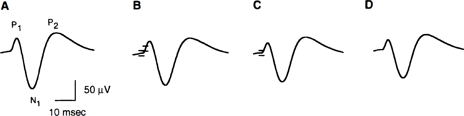
Somatosensory evoked potential (SSEP) tracings from a single characteristic rat for 2 seconds (A), 4 seconds (B), 8 seconds (C), and 16 seconds (D) stimuli. The SSEP response for all stimuli consisted on an initial positive wave (P₁) at approximately 10 milliseconds poststimulus followed by a negative (N₁) wave at approximately 13 milliseconds followed by a second positive peak (P₂) at about 17 milliseconds poststimulus. The overall magnitude of the N₁–P₂ amplitude significantly decreased with increasing stimulus duration.

TABLE 1.

SSEP values for different stimulus durations

Stimulus duration	Delay to P1 (ms)	Delay to N1 (ms)	N1–P2 amplitude (μv)	Delay to P2 (ms)
2s	9.98 ± 0.74	13.40 ± 1.22	193.8 ± 32.9	17.36 ± 1.62
4s	9.96 ± 0.57	13.22 ± 1.27	183.3 ± 40.1	17.48 ± 1.58
8s	10.07 ± 0.96	13.49 ± 0.95	171.4 ± 22.0	17.11 ± 1.33
16s	10.02 ± 0.84	13.59 ± 1.08	162.5 ± 26.4	17.60 ± 1.79

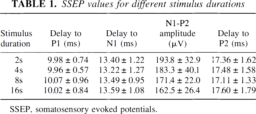
SSEP, somatosensory evoked potentials.

AFC system modeling for varying stimulus durations

Figure 3 shows the approximated neural input function n(mΔT) that was derived from the transformed N₁–P₂ amplitudes for the different stimulus durations. As seen in these figures, n(mΔT) consisted of a series of step functions at each stimulus duration. The amplitudes of these step functions were determined by linear transformation of the measured SSEP amplitudes (see Materials and Methods). It can be seen that these amplitudes decreased over time, demonstrating neural habituation.

FIG. 3.

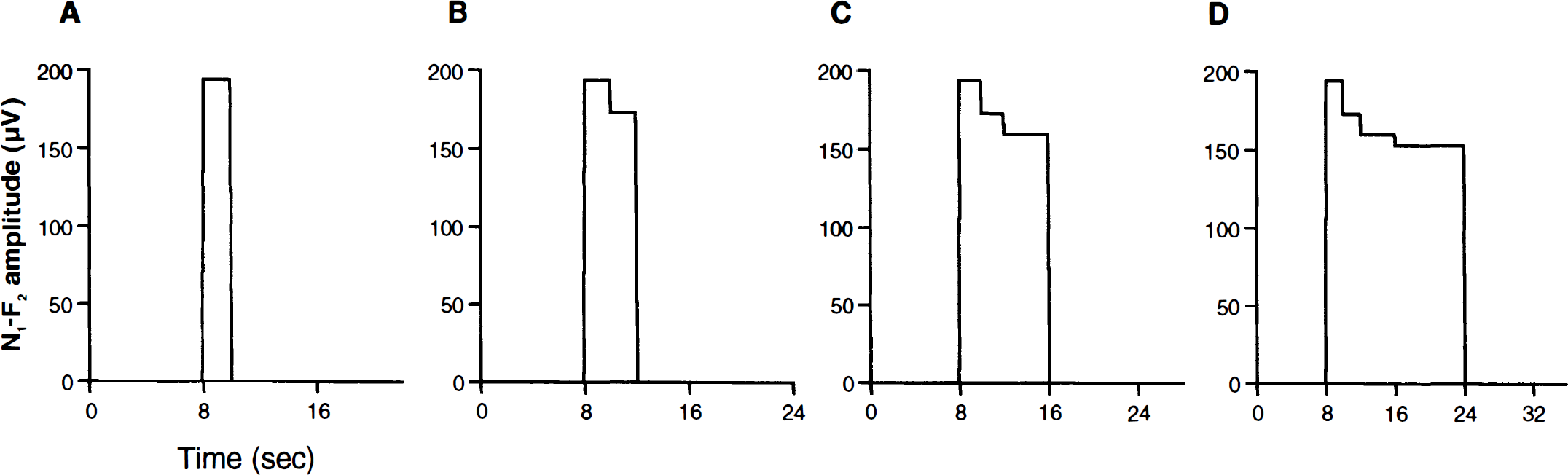
Approximated neural input functions for the different stimulus duration of 2 seconds (A), 4 seconds (B), 8 seconds (C), and 16 seconds (D) stimuli derived from transformation of the observed N₁–P₂ amplitudes.

Model 1 (Eq. 4) represents an LTI transformation of n(mΔT) to CBF. Model 2 (Eq. 6), because of the presence of a second-order kernel, can also represent non-LTI aspects of this transform. Figure 4 shows the observed LD CBF data y(mΔT) overlaid with the least-squares fits of model 1 and model 2 for variations in the stimulus duration.

FIG. 4.

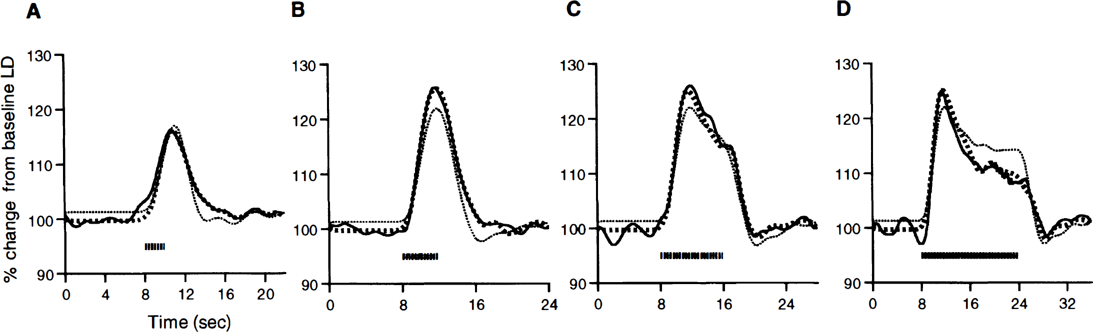
The observed cerebral blood flow (CBF) responses (solid black line) and predicted responses from Model 1 (black hatched line) and Model 2 (gray hashed line) for the different stimulus durations of 2 seconds (A), 4 seconds (B), 8 seconds (C), and 16 seconds (D) stimuli. For stimuli durations ≤ 4 seconds (A and B) both Model 1 and 2 accurately predicted the observed CBF response. However, for stimuli > 4 seconds (C and D) Model 1 overestimated the observed response especially during the plateau phase, whereas Model 2 accurately predicted the CBF responses.

As seen in Fig. 4 for the variations in the stimulus duration, model 1 does a fair job of explaining the CBF responses (r² of model 1 fit = 0.91). However, it is also evident that model 1 systematically misfits the data to an appreciable extent. This is especially evident for the longest stimulus duration (Fig. 4D) where the pure LTI model clearly overestimates the plateau phase of the response. It is provisionally concluded that an LTI model, although explaining a large amount of variance for this particular experimental manipulation, is not valid. This invalidity was not mitigated by increasing the number of basis functions used in the expansion of h¹ (mΔT) in Eq. 5 (data not shown).

The fit for model 2 for the different stimulus durations (Figs. 4A through 4D), which can accommodate some non-LTI components, is visually much better than that of model 1, especially for longer stimulus durations (Figs. 4C and 4D). Accordingly, the total amount of variability explained in the data is increased (R² of model 2 fit = 0.98). The second-order kernel parameters taken in ensemble were highly significant (F(28,59) = 5.5, P < 1E-6). This implies that the transform from neural activity (specifically, the N₁–P₂ amplitude measure of the SSEP) to CBF change is better described as nonlinear for the experimental manipulation of the stimulus duration.

Statistical significance does not convey information about the relative magnitude of the nonlinear fit contribution. Such information is conveyed by the percentage of the total variance explained by model 2, accounted for uniquely by the nonlinear components, which was 6.3%.

Study II

Qualitative effect of stimulus intensity on the CBF response

A characteristic peak change in the CBF response that was similar in shape was observed for all 4-second stimuli with different stimulus intensities (Figs. 5A through 5C). With increasing stimulus intensity, there was an increase in the peak height of the CBF response. A small increase in the systemic blood pressure was seen only at the 2 mA stimulus intensity (inset to Fig 5C). This result suggests that there could be a global blood flow effect that contaminates the corresponding local LD signal.

FIG. 5.

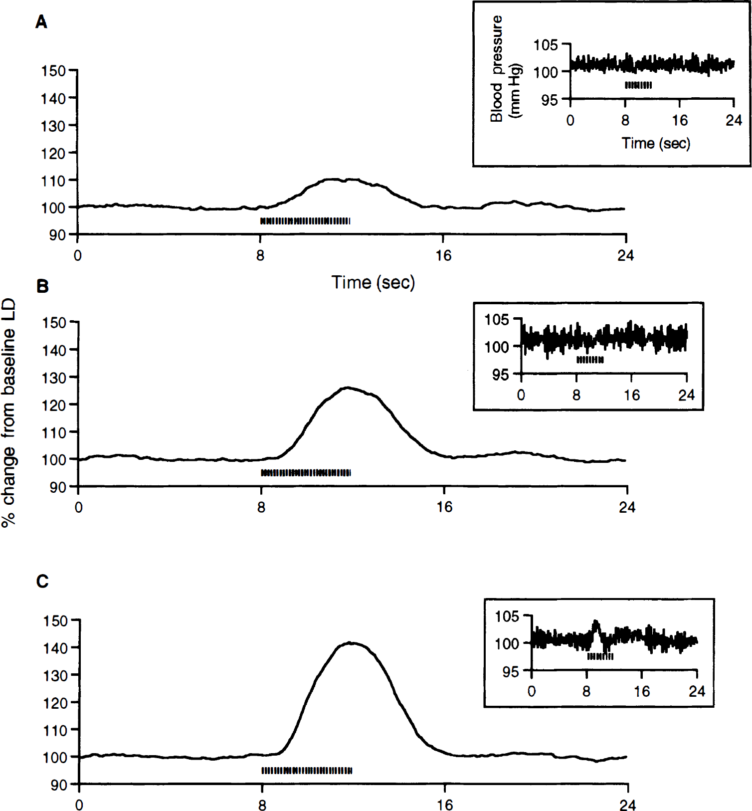
Cerebral blood flow (CBF) responses averaged over rats (n = 8) for different stimulus intensities of 0.5 mA (A), 1.0 mA (B), and 2.0 mA (C) stimuli. Insets: Average blood pressure traces for 0.5 mA (A), 1.0 mA (B), and 2.0 mA (C) stimuli. For all stimuli a peak CBF response was observed with greater stimulus intensity leading to a greater CBF response. A significant blood pressure change was also seen for 2.0 mA stimuli.

The effect of SSEP stimulus intensity on SSEP amplitude

Figure 6 shows characteristic SSEP responses averaged from a minimum of two sets of 200 evoked potentials from a single representative rat for the different stimulus intensities. P₁, N₁, and P₂ waves were observed with the various latencies not detectably varying across the different stimulus intensities (Table 2). An increase in the stimulus intensity led to an increase in the N₁–P₂ amplitude.

FIG. 6.

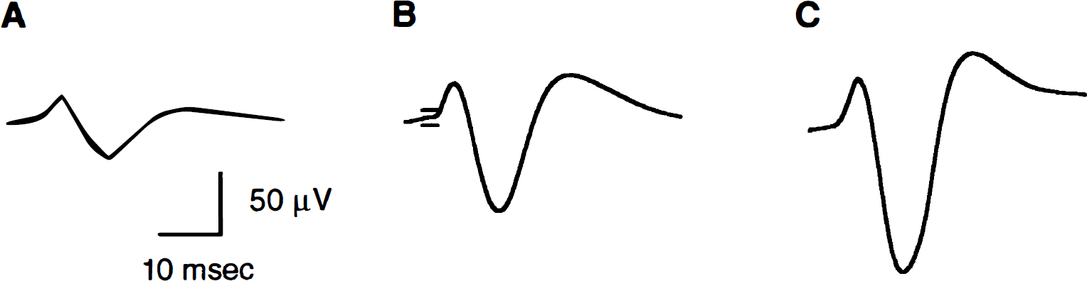
SSEP tracings from a single characteristic rat for 0.5 mA (A), 1.0 mA (B), and 2.0 mA (C) stimuli. N₁, P₁, and P₂ waves were observed with the latencies of the different peaks not effected. However, the overall magnitude of the N₁–P₂ amplitude increased with stimulus intensity. Error bars indicate SD (n = 400 SSEPs from one rat).

TABLE 2.

SSEP values for different stimulus intensities

Stimulus intensity	Delay to P1 (ms)	Delay to N1 (ms)	N1–P2 amplitude (μV)	Delay to P2 (ms)
0.5 mA	9.93 ± 054	13.19 ± 1.16	74.1 ± 23.2	17.21 ± 1.87
1.0 mA	9.97 ± 0.33	13.34 ± 1.07	177.5 ± 53.7	17.60 ± 1.94
2.0 mA	10.01 ± 0.52	13.48 ± 1.53	231.4 ± 71.5	17.58 ± 2.11

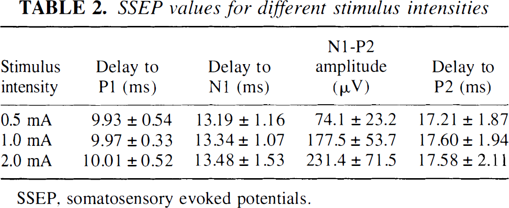
SSEP, somatosensory evoked potentials.

AFC system modeling for varying stimulus intensities

Figure 7 shows the approximated neural input function that was derived from the N₁–P₂ amplitudes for the different stimulus intensities. The amplitudes of these time series during the 4 seconds of stimulation were obtained directly from the measured SSEP amplitudes for the different stimulus intensities (Table 2).

FIG. 7.

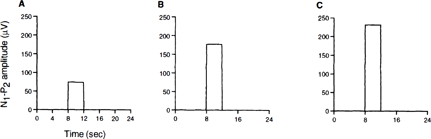
Neural input function for the different stimulus intensities of 0.5 mA (A), 1.0 mA (B), and 2.0 mA (C) stimuli derived from transformation of the observed N₁–P₂ amplitudes.

Figure 8 shows the observed LD CBF data overlaid with the least-squares fits of model 1 and model 2 for variations in the stimulus intensities. As we see in Fig. 8, model 1 does an excellent job of explaining the relationship between neural activity and CBF responses (R² of model 1 fit = 0.98). Nevertheless, the nonlinear components of model 2 provided a statistically significant contribution [F(15,40) = 4.1; P < 2E-4], albeit one small in magnitude (the percentage of the total variance explained by model 2 accounted for uniquely by the nonlinear components was 0.99%).

FIG. 8.

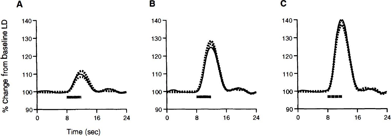
The observed CBF responses (solid black line) and predicted responses from Model 1 (black hashed line) and Model 2 (gray hashed line) forthe different stimulus intensities of 0.5 mA (A), 1.0 mA (B), and 2.0 mA (C) stimuli. For the different stimulus intensities model 1 accurately predicted the observed CBF response.

The nonlinear component seems to be mostly attributable to minor adjustments in the scaling of the CBF responses, as opposed to adjustments in the shape. A system that preserves the shape of the output, when only the scaling of the input is changed, is called time-intensity separable (Boynton et al., 1996). All LTI systems are time-intensity separable, but the converse is not true. Time-intensity separability of the AFC system for the different stimulus intensities is supported by Fig. 9, which shows the CBF responses normalized by their peak amplitudes. Furthermore, model 2 applied to the amplitude normalized data yielded a nonlinear component that uniquely accounted for only 0.13% of the total explained variance [although it was still significant because of the extremely small error variance: F(15,40) = 2.2; P = 0.03]. This demonstrates that time–intensity separability provides a superb model for the AFC system across the range of neural activity examined.

FIG. 9.

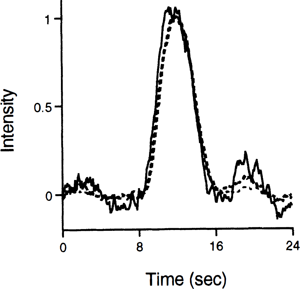
The amplitude normalized laser Doppler responses for each stimulus intensity are plotted. The evident similarity in shape of the laser Doppler responses as intensity of the neural response varies supports the time-intensity separability of the activation-flow coupling system. The solid black line represents 0.5 mA, the black hatched line represents 1.0 mA, and the gray hatched line represents 2.0 mA.

DISCUSSION

The main findings of this study are as follows: (1) although a pure LTI model explains a large amount of the variance in the data when duration of neural activity is varied, there is also a nonlinear component to the AFC system evident over this manipulation that is both statistically significant and appreciable in magnitude; and (2) an LTI approximation appears to be reasonable when the intensity of neural activity is varied and duration is kept constant, with very strong support existing for time-intensity separability of the AFC system.

In an attempt to test the hypothesis that the AFC system is LTI, we used a model that entailed several assumptions. These assumptions included (1) that N₁–P₂ SSEP amplitude was a valid measure of neural activity; (2) that there was no error in the measured SSEP amplitudes; (3) that the neural activity response was a series of rectangular pulses; (4) that any impulse response function was of less than 12 seconds duration; and (5) that the CBF time series errors were distributed as a multivariate Gaussian distribution with known autocorrelation structure. If the assumptions of our model are correct, then the LTI hypothesis should be rejected if a significant weighting on second-order kernel coefficients was observed. Our results demonstrated a significant weighting on second-order kernel coefficients when both stimulus duration and stimulus intensity were manipulated. In particular, the first-order model for longer stimulus durations (8 and 16 seconds) led to salient overestimations of the plateau phase of the LD response. Because of our use of empirical time courses of neural activity, it was shown that neural habituation could not sufficiently explain these results within the context of a linear model.

Although nonlinear components of the AFC system were deemed statistically significant when both stimulus duration and stimulus intensity were manipulated, the magnitude of the relative nonlinear contribution was more than six times greater for the duration manipulation compared with intensity manipulation. Furthermore, when amplitude-normalized data were considered, this value increases to 48. This, coupled with the high absolute explanatory power of the pure LTI model for the intensity manipulation (R² of model 1 fit = 0.98), supports the validity of the use of an LTI approximation for variations of intensity, but not duration, of neural activity.

A detail to be considered is the interpretation of the small but statistically significant nonlinear component of the AFC system that was observed in study II. A possible explanation for this result is related to measurement errors of the SSEPs. Our use of approximate neural activity functions to characterize the AFC system involved two assumptions. One is that the actual neural activity responses were rectangular pulses of several seconds in duration. Given the relatively small degree of habituation in neural response over time (as seen in study I), this first assumption seems a reasonable approximation. The second assumption was that the measured SSEPs were without error. As seen from our measurements in Table 2, this is incorrect. The consequence of using an independent variable with error in our statistical modeling framework is to bias both our estimates of the AFC system parameters, as well as bias our estimates of their variability (Schoukens and Pintelon, 1991). Appropriate statistical “error-in-the-variables” models could be used for consideration of such problems. When using our method, however, bias in the statistical inference is small when the “error-in-the-variables” is small relative to the unexplained variance in the dependent data. So, we presumed that using a more standard (and more easily implementable and communicable) statistical model than an error-in-the-variables model would be a tenable approach. But, given the post hoc observation that the LD time series error was so low in study II (Fig. 8), it now seems reasonable to postulate that our result of a statistically significant non-linear AFC component in study II is an artifact because of error in the SSEP measurements. If this were true, then averaging of more SSEP trials should make the non-linear contribution even smaller. In any case, the magnitude of the nonlinear contribution in study II was less than 1% of the total variance explained by the AFC system. Furthermore, the same hypothesis would not explain the statistically significant nonlinear component in study I, because both its magnitude is greater than in study II and the CBF time series error is greater in study I (owing to 10 times fewer trials being used; see Materials and Methods).

Despite the strong evidence against the validity of an LTI model when duration is manipulated, it is still worth considering that in terms of the magnitude of variance explained (R² of model 1 fit = 0.91), the pure LTI model fared reasonably well in study I. To state that a model is invalid, but also claim that it is a reasonable approximation is not equivocation. A model can be invalid in an absolute sense, but still be useful in situations where sensitivity to violations of the model is low. Given our results, an example of such a case would be the use of alterations in CBF simply as a measure of the presence or the absence of neural activity at various durations after stimulation onset. In such a case, one could use the LTI model to generate predictions, which would be correct in an ordinal sense but not in a quantitative sense. An example of a case where our results would imply that an LTI model would not be valid would be where one wishes to make accurate measures of the time course of neural habituation with CBF.

Our results of a generally good LTI approximation to the AFC system are similar to previous animal studies (Mathiesen et al., 1998; Ngai et al., 1999) that have attempted to clarify the relationship between integrated neuronal activity and the peak (Mathiesen et al., 1998) or time-averaged (Ngai et al., 1999) CBF response. In these studies, integrated field potentials were used as a measure of neural activity and were compared with summary measures of CBF responses. For both studies, a linear transformation was observed when the stimulus frequency was varied. In contrast to those experiments, in this study, we preserved the CBF time series. Using the entire time course (instead of only summary measures) allowing for a more complete test of the LTI assumption. This analysis permitted us to explicitly model a second-order kernel and demonstrate approximately linear behavior, as well as make more fine-grained nonlinear characterizations of the transform.

Our observed results may have important implications for future analysis of functional magnetic resonance imaging (fMRI) studies. Several authors of fMRI studies have investigated the linearity of the blood oxygenation level-dependent (BOLD) hemodynamic response to different stimuli (Boynton et al., 1996; Cohen, 1997; Dale and Buckner, 1997; Friston et al., 1998; Rees et al., 1997; Vazquez and Noll, 1998). Boynton et al. (1996) demonstrated that an LTI model provides a reasonable approximation for the observed BOLD-fMRI signal by using simple visual checkerboard stimuli. Some deviations from linearity between the stimulus duration and the BOLD response were observed with longer stimuli but were hypothesized to be the result of neural adaptation. However, our results suggest that neural habituation cannot fully explain the observed nonlinearities. In another study of linearity, Dale and Buckner (1997) assessed the superposition of overlapping BOLD responses in the occipital cortex because of closely spaced visual stimuli. These authors demonstrated that if trial types are randomly mixed and selective averaging is performed on the trial types, the BOLD hemodynamic response can be ascertained from stimuli as little as 2 seconds apart.

However, several fMRI studies have also demonstrated nonlinear aspects of the BOLD response. Vazquez and Noll (1998) have demonstrated nonlinearities in the BOLD response in the visual system when the stimulus duration and contrast were varied with the strongest nonlinearities observed with manipulation of the stimulus duration. These observations are very similar to results that we have observed in this study. Both Rees et al. (1997) and Friston et al. (1998) have also demonstrated for positron emission tomography that CBF was linear with respect to variations in auditory stimulus frequency, whereas the BOLD response was nonlinear. More recently, the linearity of the CBF response, using arterial spin labeling technique and BOLD, have been examined by using a motor task of different durations (Miller et al., 1999). These authors demonstrated that, for brief stimuli in the range of 2 to 18 seconds, the arterial spin labeling response was linear with respect to motor task duration, whereas the BOLD effect was not linear. For all of the above neuroimaging studies, the linearity transformation has been analyzed with respect to an assumed neural activity waveform that bore a simple relationship to stimulation parameters. Future studies in humans that measure both neuronal activity and hemodynamic response would allow a more accurate characterization of the AFC system and BOLD-fMRI systems.

Footnotes

Abbreviations used

References

Ances

Detre

Takahashi

Greenberg

(1998) Transcranial laser Doppler mapping of activation flow coupling of the rat somatosensory cortex. Neurosci Lett 257:25–28

Bandettini

Wong

Hinks

Tikofsky

Hyde

(1992) Time course EPI of human brain function during task activation. Magn Reson Med 25:390–397

Bendat

(1990) Non-linear system analysis and identification from random data. New York, NY: John Wiley.

Bonvento

Charbonne

Correze

Borredon

Seylaz

Lacombe

(1994) Is alpha-chloralose plus halothane induction a suitable anesthetic regimen for cerebrovascular research? Brain Res 665:213–221

Boynton

Engel

Glover

Heeger

(1996) Linear systems analysis of functional magnetic resonance imaging in human VI. J Neurosci 16:4207–4221

Cohen

(1997) Parametric analysis of fMRI data using linear systems methods. Neuroimage 6:93–103

Dale

Buckner

(1997) Selective averaging of rapidly presented individual trials using fMRI. Hum Brain Mapping 5:329–340

Detre

Ances

Takahashi

Greenberg

(1998) Signal averaged laser Doppler measurements of activation-flow coupling in the rat forepaw somatosensory cortex. Brain Res 796:91–98

Barth

(1991) Topographic analysis of field potentials in rat vibrassae/barrel cortex. Brain Res 546:106–112

10.

Dirnagl

Lindauer

Villringer

(1993) Role of nitric oxide in the coupling of cerebral blood flow to neuronal activation in rats. Neurosci Lett 149:43–46

11.

Dirnagl

Niwa

Lindauer

Villringer

(1994) Coupling of cerebral blood flow to neuronal activation: role of adenosine and nitric oxide. Am J Physiol 267:H296–H301

12.

Friston

Frith

Frackowiak

Turner

(1995a) Characterizing dynamic brain responses with fMRI: a multivariate approach. Neuroimage 2:166–172

13.

Friston

Frith

Turner

Frackowiak

(1995b) Characterizing evoked hemodynamics with fMRI. Neuroimage 2:157–165

14.

Friston

Holmes

Poline

Grasby

Williams

Frackowiak

Turner

(1995c) Analysis of fMRI time-series revisited. Neuroimage 2:45–53

15.

Friston

Jezzard

Turner

(1994) Analysis of functional fMRI time series. Hum Brain Mapping 1994;1:153–171

16.

Friston

Josephs

Rees

Turner

(1998) Nonlinear event-related responses in fMRI. Magn Reson Med 39:41–52

17.

Johnston

(1972) Econometrics methods. New York, NY: McGraw-Hill Josephs O, Henson RN (1999) Event-related functional magnetic resonance imaging: modeling, inference and optimization. Philos Trans R Soc Lond B Biol Sci 354:1215–1228

18.

Lindauer

Megow

Schultze

Weber

Dirnagl

(1996) Nitric oxide synthase inhibition does not affect somatosensory evoked potentials in the rat. Neurosci Lett 216:207–210

19.

Mathiesen

Caesar

Akgoren

Lauritzen

(1998) Modification of activity-dependent increases of cerebral blood flow by excitatory synaptic activity and spikes in rat cerebellar cortex. J Physiol (Lond) 512:555–566

20.

Mathiesen

Caesar

Lauritzen

(2000) Temporal coupling between neuronal activity and blood flow in rat cerebellar cortex as indicated by field potential analysis. J Physiol (Lond) 523:235–246

21.

Miller

Buxton

Wong

Frank

(1999) The linearity of the cerebral blood flow response to brief motor tasks. ISMRM Abstr. 381

22.

Narayan

Santori

Blood

Burton

Toga

(1994) Imaging optical reflectance in rodent barrel and forelimb sensory cortex. Neuroimage 1:181–190

23.

Ngai

Jolley

D'Ambrosio

Meno

Winn

(1999) Frequency-dependent changes in cerebral blood flow and evoked potentials during somatosensory stimulation in the rat. Brain Res 837:221–228

24.

Ngai

Winn

(1995) Modulation of cerebral arteriolar diameter by intraluminal flow and pressure. Circ Res 1995;77:832–840

25.

Ogawa

Lee

Kay

Tank

(1990) Brain magnetic resonance imaging with contrast dependent on blood oxygenation. Proc Natl Acad Sci U S A 87:9868–9872

26.

Ogawa

Tank

Menon

Ellermann

Kim

Merkle

Ugurbil

(1992) Intrinsic signal changes accompanying sensory stimulation: functional brain mapping with magnetic resonance imaging. Proc Natl Acad Sci U S A 89:5951–5955

27.

Oppenheim

Willsky

Young

(1983) Signals and systems. Englewood Cliffs, NJ: Prentice-Hall

28.

Rees

Howseman

Josephs

Frith

Friston

Frackowiak

Turner

(1997) Characterizing the relationship between BOLD contrast and regional cerebral blood flow measurements by varying the stimulus presentation rate. Neuroimage 6:270–278

29.

Schoukens

Pintelon

(1991) Identification of linear systems. New York, NY: Pergamon Press

30.

Vazquez

Noll

(1998) Nonlinear aspects of the BOLD response in functional MRI. Neuroimage 7:108–118

31.

Worsley

Friston

(1995) Analysis of fMRI time-series revisited—again [comment]. Neuroimage 2:173–181

Coupling of Neural Activation to Blood Flow in the Somatosensory Cortex of Rats is Time-Intensity Separable,but Not Linear

Abstract

Keywords

MATERIALS AND METHODS

Surgical preparation

Forepaw stimulation

Experimental stimulation protocols

Study I

Study II

Data analysis of CBF measurements by using LD

Somatosensory evoked potentials

Determination of the amplitude of neural activity during the stimulus time periods

Modeling of the AFC system

RESULTS

Physiologic variables

Study I

Qualitative effect of stimulus duration on the CBF response

SSEP measurements for different stimulus durations

AFC system modeling for varying stimulus durations

Study II

Qualitative effect of stimulus intensity on the CBF response

The effect of SSEP stimulus intensity on SSEP amplitude

AFC system modeling for varying stimulus intensities

DISCUSSION

Footnotes

Abbreviations used

References