Cerebral Blood Flow Measurements by Magnetic Resonance Imaging Bolus Tracking: Comparison with [ 15 O]H 2 O Positron Emission Tomography in Humans

Abstract

In six young, healthy volunteers, a novel method to determine cerebral blood flow (CBF) using magnetic resonance (MR) bolus tracking was compared with [¹⁵O]H₂O positron emission tomography (PET). The method yielded parametric CBF images with tissue contrast in good agreement with parametric PET CBF images. Introducing a common conversion factor, MR CBF values could be converted into absolute flow rates, allowing comparison of CBF values among normal subjects.

Recent results indicate that it may be possible to measure CBF by dynamic magnetic resonance imaging (MRI) of paramagnetic contrast agent bolus passage (Østergaard et al., 1996a). Because of the complexity of susceptibility contrast, this technique initially only allowed determination of relative flow rates. In a preliminary study in six normal volunteers, the mean gray to white flow ratio was found to be in good agreement with PET literature values for age-matched subjects (Østergaard et al., 1996b). In a recent animal hypercapnia study (Østergaard et al., 1998), an approach was introduced to allow absolute quantitation by introduction of an empirical normalization constant.

In this study, we compare absolute regional MR bolus tracking CBF values with CBF values determined by [¹⁵O] water uptake, detected by positron emission tomography (PET), in normal human volunteers.

THEORY

Magnetic resonance imaging cerebral blood flow measurements

Estimation of CBF from measurement of nondiffusable tracers is discussed in detail by Østergaard et al. (1996a). In brief, the concentration C_t(t) of intravascular contrast agent within a given tissue element can be written:

$$C_t(t)=F_t\cdot C_a(t)\otimes R(t)$$

(1)

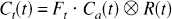
where F_t is tissue flow and ⊗ denotes the convolution of R(t), the vascular residue function (normalized impulse response function) with the arterial input function, C_a(t). It has been demonstrated that, using singular value decomposition (SVD), R(t) and CBF can be determined with good accuracy, independent of the underlying vascular structure and volume (Østergaard et al., 1996a). The MR measurements of tissue tracer concentration are made with an imaging sequence sensitive to small, capillary size vessels (Fisel et al., 1991; Weisskoff et al., 1994), so that the concentration term in equation 1 mainly reflects that of capillaries (see below).

Positron emission tomographic cerebral blood flow measurement

The regional uptake of water is described by the model of Ohta et al. (1996):

$$C_{br}(t)=(1-V_p)\cdot K_1\cdot {\int }_0^t{C}_a(\tau )e^{-k_2(t-\tau )}d\tau +V_p\cdot C_a(t)$$

(2)

where we assume K₁ = CBF for water, and k ₂ = K ₁ /V _d , where V_d is the distribution volume of the tracer. V_p is the instantaneous vascular distribution volume of the tissue.

MATERIAL AND METHODS

Volunteers and experimental protocol

Six young, healthy volunteers (3 men, 3 women, mean age 26 ± 6 years) were examined. Two additional volunteers were originally included in the study. One was excluded owing to head motion during MRI measurements, while the other was excluded because of a significant change (>5%) in PaCO₂ in between PET and MR scans. PET and MR scans were performed on the same day, within 2 hours of each other. Before the examination, arterial and venous catheters were inserted in the left radial artery and right antecubital vein, respectively. Arterial blood samples were withdrawn and analyzed (ABL 300, Radiometer, Copenhagen) at regular intervals to monitor blood gases and whole blood acid-base parameters (pH, P_aCO₂, PaO₂, HCO₃, and O₂ saturation). Before each CBF measurement, the volunteer was allowed to rest at least 30 minutes with closed eyes. The project was approved by the Regional Danish Committee for Ethics in Medical Research, and performed after informed, written consent from each volunteer.

Positron emission tomographic imaging protocol

The volunteers were studied in a Siemens ECAT EXACT HR PET camera (Siemens/CTI, Knoxville, TN, U.S.A.) using a custom-made head-holding device. To measure CBF, a fast intravenous bolus injection of 500 MBq[¹⁵O]H₂O in 5 mL saline was performed, followed immediately by an intravenous injection of 10 mL of isotonic saline to flush the catheter. A sequence of 21 (12, 6, and 3 samples during the first, second, and third minute, respectively) arterial blood samples (1 to 2 mL) and 12 PET brain images (6, 4, and 2 images per minute, respectively) were then obtained. Brain image data were reconstructed using scatter correction and a Hanning filter with a cutoff frequency of 0.5 pixel⁻¹, resulting in an isotropic spatial resolution (full width at half maximum) of 4.6 mm. Correction for tissue attenuation was based on a ⁶⁸Ga transmission scan. Radioactivity levels in image and arterial blood were corrected for the half-life of ¹⁵O (123 seconds).

Positron emission tomographic radiochemistry

¹⁵O₂ was produced by the ¹⁴N(d,n)¹⁵O nuclear reaction by the bombardment of nitrogen gas with 8.4 MeV deuterons using a GE PETtrace 200 cyclotron (GE Medical Systems, Uppsala, Sweden). ¹⁵O₂ was mixed with hydrogen and passed in a stream of nitrogen gas over a palladium catalyst at 150°C to produce ¹⁵O-water vapor, which was trapped in 10 mL sterile saline.

Magnetic resonance imaging protocol

Magnetic resonance imaging was performed using a GE Signa 1.0 Tesla imager (GE Medical Systems, Milwaukee, WI, U.S.A.). After a sagittal scout, a T₁-weighted three-dimensional image was acquired for coregistration of MR and PET data. For dynamic imaging of the bolus passages, spin echo-planar imaging(EPI) was performed (repetition time, TR = 1,000 milliseconds; echo time, TE = 75 milliseconds), using a 64 by 64 acquisition matrix with an 18- by 18-cm transverse field of view, leading to an in-plane resolution of 3 by 3 mm. The slice thickness was 6 mm. In all experiments, bolus injection of 0.2 mmol/kg gadodiamide (Gd-DTPA-BMA, OMNISCAN, Nycomed Imaging, Oslo, Norway) was performed at a rate of 5 mL/second. A predose of 0.05 mmol/kg was given to reduce systematic effects from changes in blood T₁.

Magnetic resonance image analysis

To determine tissue and arterial tracer levels C(t), we used susceptibility contrast (Villringer et al., 1988) arising from compartmentalization of the paramagnetic contrast agent. We assumed a linear relationship (Weisskoff et al., 1994) between paramagnetic contrast agent concentration and the change in transverse relaxation rate ΔR₂:

$$C(t)\propto \Delta R_2(t)=-log\left(\frac{S(t)}{S(0)}\right)/\text{TE}$$

(3)

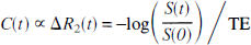
where S(0) and S(t) are the signal intensities at the baseline and at time t, respectively, and TE the echo time. The arterial concentration was determined from pixels within the middle cerebral artery in the imaging plane (Porkka et al., 1991). The integrated area of the arterial input curve in each measurement was normalized to the injected contrast dose (in millimoles per kilogram body weight) according to our earlier approach (Østergaard et al., 1998). Deconvolution of the measured tissue (equation 1) by SVD was performed after the application of a 3 × 3 uniform smoothing kernel to the raw image data, and CBF was determined as the height of the deconvolved tissue curve.

Positron emission tomographic image analysis

The three-dimensional PET CBF images were automatically coregistered with the three-dimensional MR images (Collins et al., 1994). Raw PET image data were then transformed and resampled to the same spatial location and resolution as the MR CBF data to allow direct comparison of the two techniques. After the application of a 3 × 3 uniform smoothing kernel to our raw PET image data, these were fitted to equation 2 using nonlinear, least squared regression analysis on a pixel-by-pixel basis.

Comparison of positron emission tomographic and magnetic resonance parametric images

Pixel-by-pixel maps of CBF (at similar anatomic locations, pixel size and resolution generated by PET and MR, respectively) were then compared on a regional basis. In each image, 20 to 25 regions of similar size were chosen, including gray and white matter. The means of all regional values were then averaged, to yield a common conversion factor between MRI flow units and absolute flow in mL · 100 mL⁻¹ · minute⁻¹). Regional average CBF values and their standard deviations (derived from the population of pixels within the region of interest [ROI]) were then compared.

RESULTS

Table 1 shows values of P_aco₂ and P_ao₂ for all volunteers during MR and PET measurements. Volunteer 3 showed a 13% change in P_aco₂ and was excluded from the analysis, whereas volunteer 1 had to be excluded because of head motion during the MR measurements.

Table 1

Blood gas levels during PET and MR CBF measurements

	Paco2 (kPa)			Pao2 (kPa)
Subject No.	PET	MR	% change	PET	MR	% change
1	5.97	5.63	−5.7	12.11	13.45	4.8
2	5.49	5.35	−2.5	15.815	16.395	3.7
3	6.63	5.79	12.7	12.05	12.625	4.8
4	5.31	5.33	0.4	15.58	16.165	3.8
5	5.25	5.325	1.4	17.175	15.265	−11
6	4.92	4.93	0.2	15.165	14.67	−3
7	4.485	4.675	4.2	15.925	16.97	6.6
8	4.965	4.965	0	16.16	15.205	−5.9

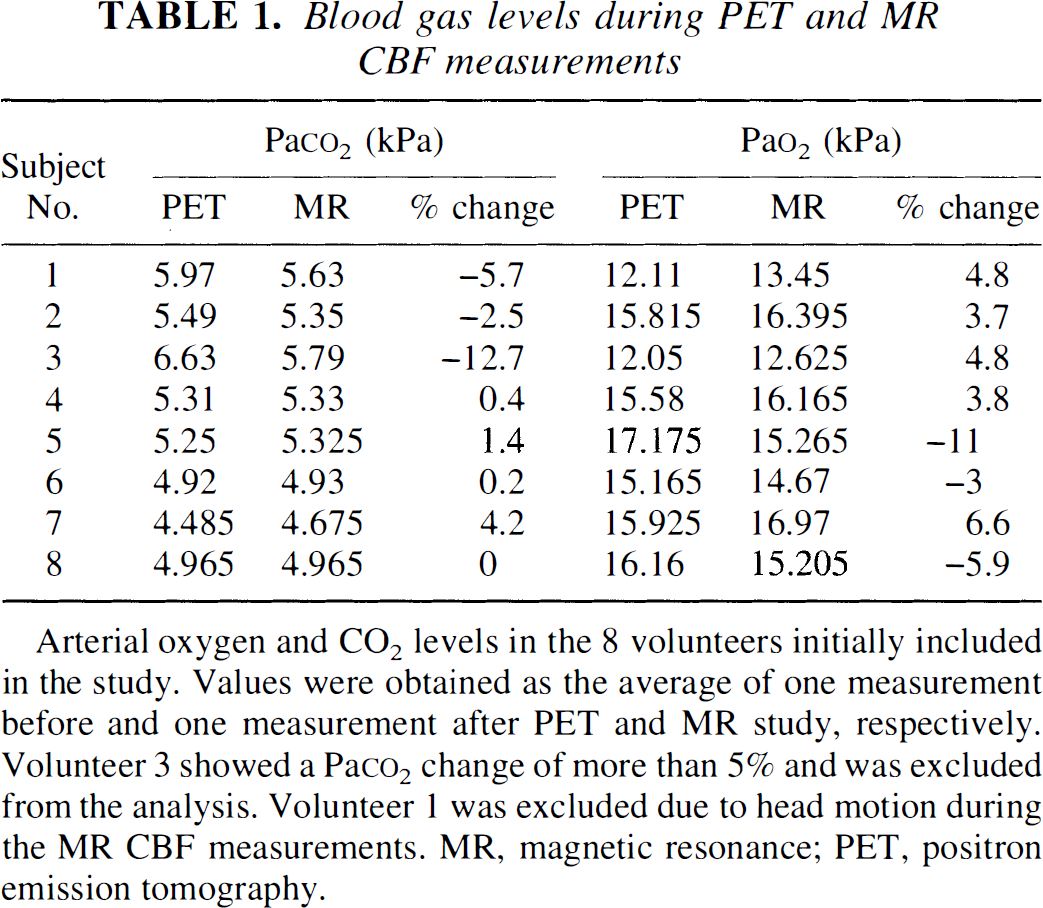
Arterial oxygen and CO₂ levels in the 8 volunteers initially included in the study. Values were obtained as the average of one measurement before and one measurement after PET and MR study, respectively. Volunteer 3 showed a Paco₂ change of more than 5% and was excluded from the analysis. Volunteer 1 was excluded due to head motion during the MR CBF measurements. MR, magnetic resonance; PET, positron emission tomography.

By averaging all regional flow rates, a common conversion factor, Φ_Gd = 0.87 was found. In the following, all MR flow rates were multiplied by this constant.

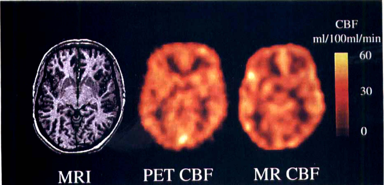
Fig. 1 shows parametric CBF maps determined by PET and NMR. To facilitate visual comparison, the MR flow image was blurred to the resolution of the PET image. Also shown is the corresponding anatomic MR image. Areas in close relation to vessels appear to have high flow rates on the MR CBF maps, whereas this was not the case in the PET CBF maps. We will discuss these methodological differences below. Fig. 2 shows MR versus PET plots of regional CBF values along with their standard deviations for the six volunteers. Also shown are linear regression lines and their 95% confidence regions. White matter ROI are represented in the lower left quadrant of the plots, whereas gray matter ROI are in the upper right. There was no systematic deviation from the regression lines for gray and white matter flow rates, in agreement with the qualitative appearance of the flow maps in Fig. 1. Also, notice that error bars are of comparable size for PET and MR for identical size ROI. Table 2 shows the regression results. The portion of the variance accounted for by the regression (r²), was generally between 65% and 83% (see Table 2). To test whether the differences in regression slopes could be ascribed to individual uncertainties, the F statistic was calculated, showing no significant differences. Still, it was noticed that subject 5 had a somewhat larger slope than the remaining volunteers. In one volunteer (subject 8), we found an apparent hypoperfusion in the occipital lobe not visible in the PET CBF image (Fig. 3). We will discuss the implications of this below.

Table 2

Linear regression results from Fig. 2

Subject	Slope (mi ± si)	Intercept	r2
2	1.09 ± 0.17	6.88 ± 5.17	0.65
4	1.08 ± 0.14	−0.48 ± 3.58	0.77
5	1.34 ± 0.17	−6.84 ± 4.21	0.74
6	1.01 ± 0.10	−10.86 ± 5.92	0.83
7	1.12 ± 0.12	1.73 ± 3.29	0.79
8	0.94 ± 0.14	2.41 ± 6.42	0.66
Mean	1.10 ± 0.14	−1.19 ± 6.51	0.74

$$F=\frac{\sum _{i=1}^N{(m_i-m_o)}^2/(N-1)}{\left(\sum _{i=1}^N{s}_i^{2}d{f}_i/\sum _1^{N}d{f}_i\right)}=0.99\hspace{0.17em}\hspace{0.17em}\hspace{0.17em}\hspace{0.17em}\hspace{0.17em}\text{NS}$$

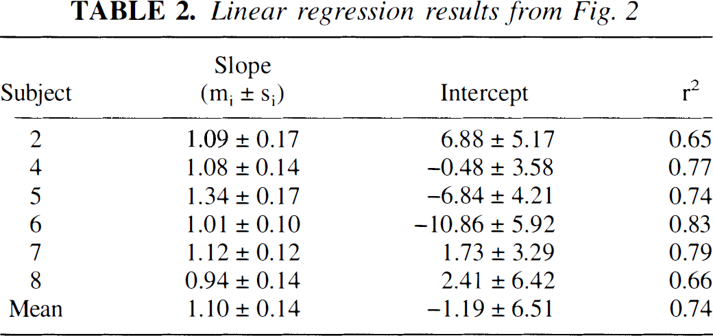
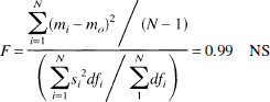
Slopes and y intercepts determined by linear regression analysis of the MR versus PET regional CBF plots in Fig. 2. Also shown is r², the proportion of variance accounted for by the linear regression. The ratio of group to individual variance was also calculated, with N = 6, where m_i and s_i are the means and standard errors of the regression line slopes, m₀ the mean slope, and df_i the degrees of freedom in each regression Number of ROI minus 2). The F implied that differences in slopes can be ascribed to uncertainties in measurements of individual slopes. MR, magnetic resonance; PET, positron emission tomography; ROI, regions of interest.

FIG. 1.

Comparison of PET and MR parametric CBF images in subject 8, after blurring the MR CBF image to the resolution of the PET CBF. Also shown is the corresponding slice on the T₁-weighted MR image. MR and PET slices are at identical locations and have identical pixel volumes. MR, magnetic resonance; PET, positron emission tomography.

FIG. 2.

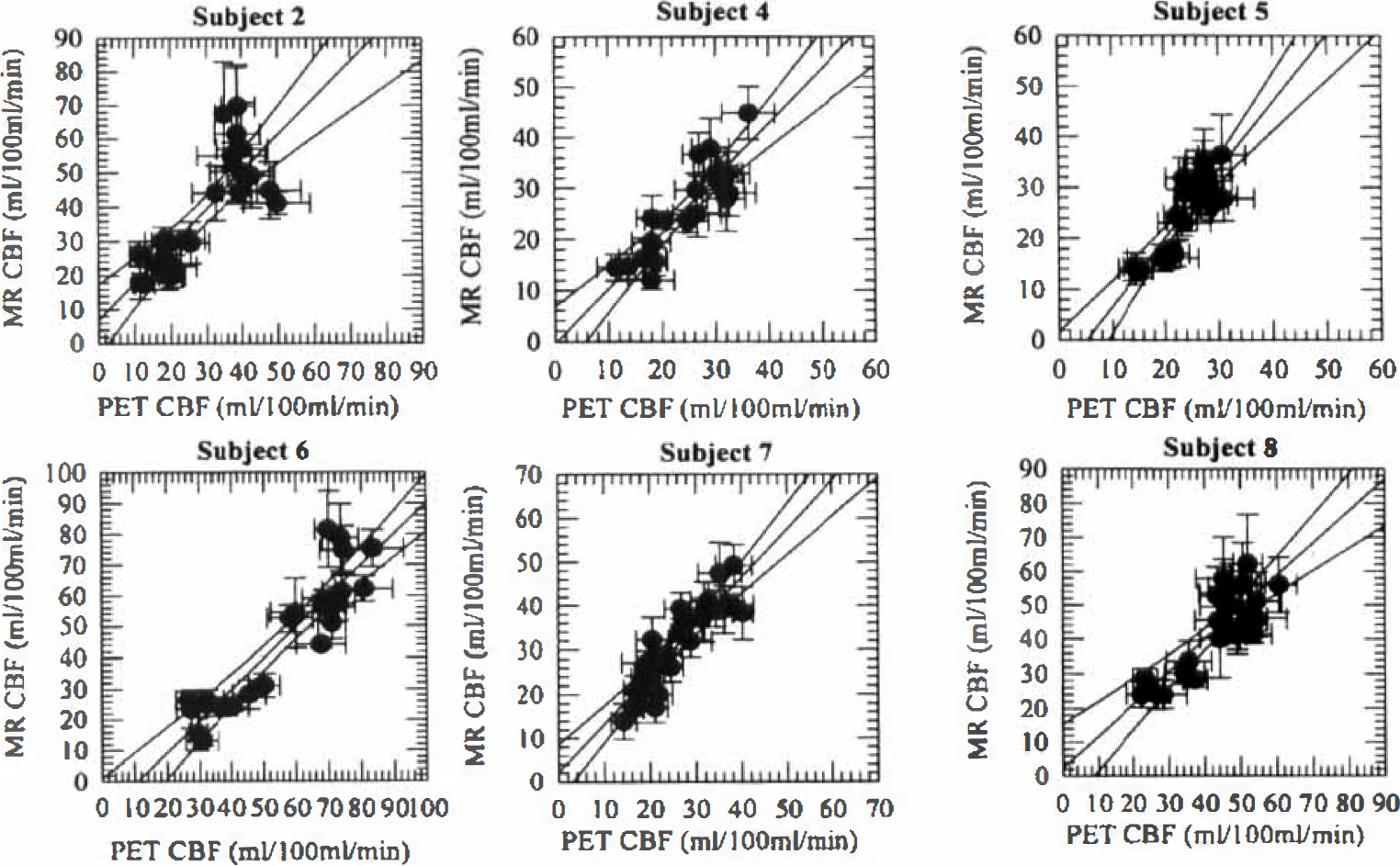
Comparison of regional PET and MR CBF values for each subject. Notice that gray and white matter ROI are separated in most subjects. Also, error bars are of comparable sizes for most regions. MR, magnetic resonance; PET, positron emission tomography; ROI, region of interest.

FIG. 3.

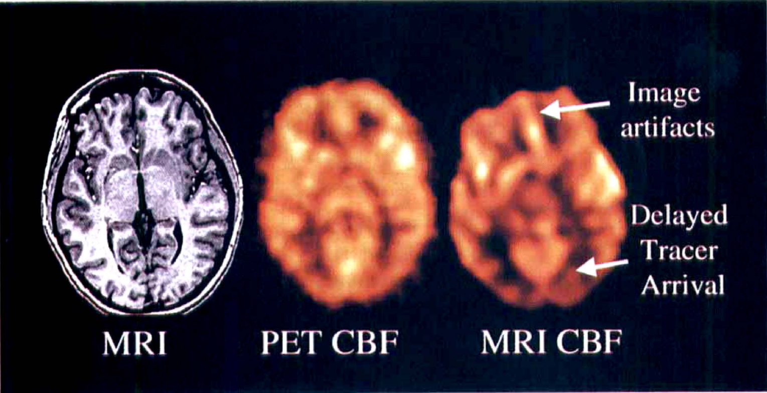
CBF images from volunteer 6. Notice that the frontal region is somewhat distorted in the MR CBF map, probably because of inhomogeneities arising from the air-tissue interfaces in the frontal sinuses. The flow rates are relatively small in the areas supplied by the posterior circulation, probably because of delayed tracer arrival. MR, magnetic resonance; PET, positron emission tomography.

DISCUSSION

There was generally good agreement between regional PET and MR CBF values. The fact that the ratio of gray and white matter flow rates appears identical using MR and PET confirms the earlier finding that relative CBF values can be determined within the same subject (Østergaard et al., 1996b). Furthermore, the data support the conclusion that our earlier normalization routine (Østergaard et al., 1998) allows determination of absolute flow rates and hence comparison among subjects. The conversion factor we found (0.87) was somewhat lower than that previously found for pigs (1.09) (Østergaard et al., 1998). We ascribe this to anatomic differences, especially the fact that the portion of the cardiac output distributed to the brain is probably smaller in pigs than in humans.

The variance observed when comparing CBF estimates obtained by PET and MR can be ascribed to several factors. In the following, we will discuss these in terms of the methodological differences between the two techniques.

Duration of cerebral blood flow measurement

Apart from CBF changes caused by overall differences in the level of consciousness between measurements (these were separated by 2 hours), the PET and MR bolus tracking techniques differ in terms of the duration of data acquisition. To observe the distribution of diffusible tracers (in our case radiolabeled water) for our PET CBF measurements, the tissue uptake must be observed for at least 3 minutes. In contrast, the duration of an intravascular bolus passage is only about 15 seconds. Because regional flow rates are unlikely to be constant over even very short time scales, this may contribute to differences in regional values.

Anatomic precision

Technical and methodological issues may have affected our measurements as well. The rapid EPI sequence used in our measurements is sensitive to magnetic field inhomogeneities. This causes geometric distortions of the MR images, and may result in misregistration of corresponding PET and MRI regions. This is illustrated in Fig. 3, displaying the conventional MRI as well as the PET CBF maps from volunteer 6. One examination had to be discarded owing to subject head motion. The sensitivity to motion arises from the fact that tracer concentrations in MR are derived from 10% to 15% signal drops (equation 3) rather than the appearance of a tracer signal on a zero background, as one sees in PET. This drawback is partially compensated by the short duration of the study.

Sensitivity to tracer arrival delays

Fig. 3 also shows what may be a reflection of a methodological problem of the MR technique. The MR technique is sensitive to large delays in tracer arrival, causing CBF to be somewhat underestimated (Østergaard et al., 1996a). In this volunteer, the tracer arrival in the posterior circulation was delayed by several seconds relative to its arrival in the remaining brain. This, apart from possible differences in visual activity during the two measurements, may explain the apparent occipital hypoperfusion in this volunteer. We compared the sensitivity of PET and MR bolus tracking CBF measurements in a simple simulation experiment by introducing delays between the arterial and cerebral concentration time curves in volunteer 6 before CBF analysis. Fig. 4 shows how flow estimates become increasingly underestimated as the arrival delay of the tracer at a brain region increases, in both PET and MR CBF measurements. Notice, however, that whereas PET measurements may underestimate flow by 15%, underestimation by MRI can be as much as 50%. Even though we only noticed this effect in one volunteer, these simulations underline the importance of further evaluating this technique in patient populations with vascular diseases. We are currently working on approaches to minimize the sensitivity of our CBF algorithm to tracer arrival delays.

FIG. 4.

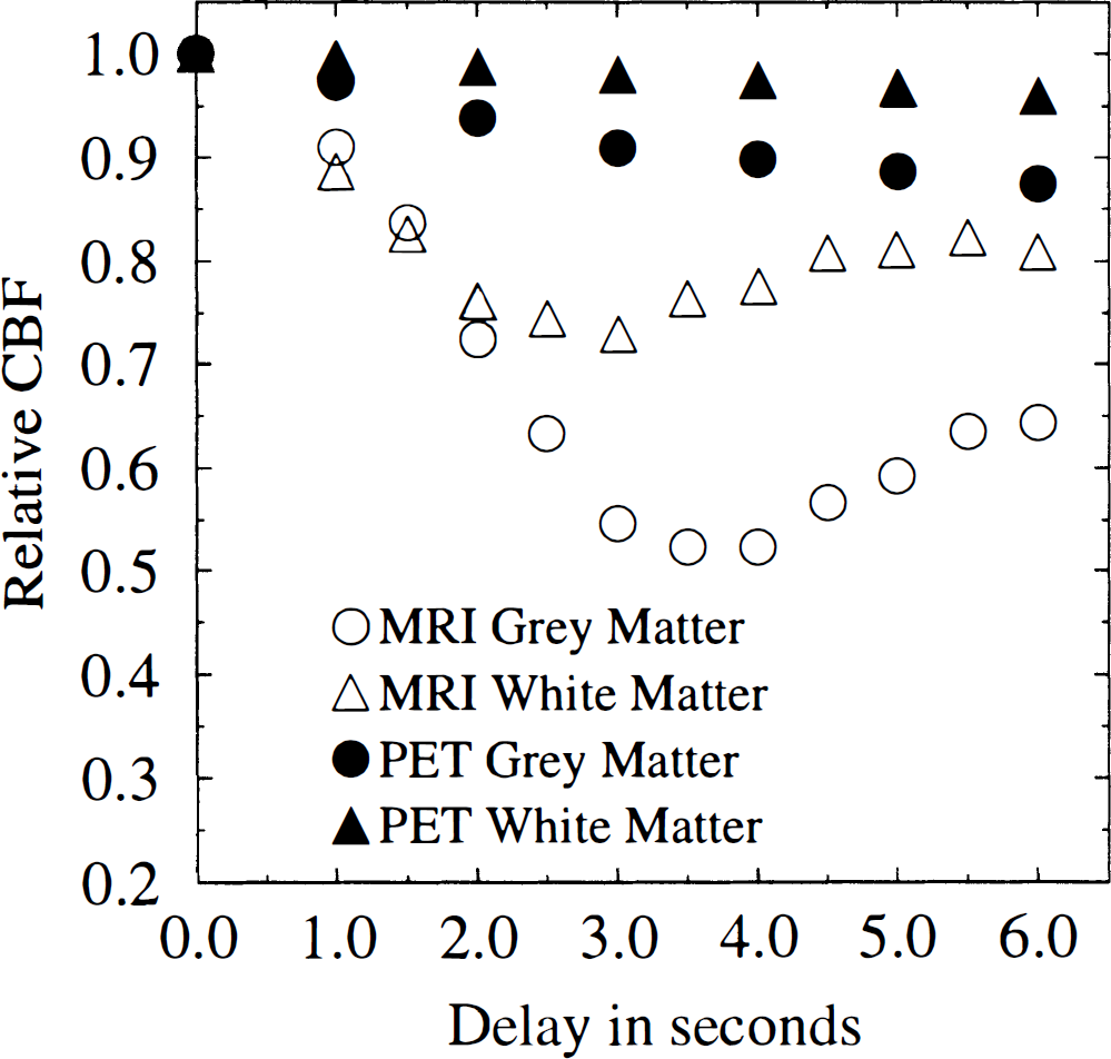
Relative flow rates as a function of increasing delays between arterial and cerebral concentration-time curves in volunteer 6. Results are normalized relative to a zero delay. For the PET measurement, this delay was fitted by nonlinear least squared regression analysis of the whole head tissue concentration curve. For MR measurements, results are relative to an assumed zero delay. Notice that errors are larger in gray than white matter for both MRI and PET. MRI, magnetic resonance imaging; PET, positron emission tomography.

Sensitivity to major vessels

The MR bolus tracking technique was found to interpret some regions with vessel branches as areas of high flow. This is inherent to the technique, as the operational equation (equation 1) does not mathematically distinguish dispersion taking place in large vessels from capillary tracer retention. However, because cerebral blood volume is simultaneously determined by integration of the tissue concentration-time curve (Rosen et al., 1990, 1991), this does not pose a problem in interpreting the CBF maps. Also, because of the inherent sensitivity of susceptibility contrast imaging to small vessels (Fisel et al., 1991; Weisskoff et al., 1994), most effects from large vessels are suppressed in the images. In the dynamic [¹⁵O] water PET experiments, a substantial vascular signal is detected right after the bolus injection. However, because of the differences between the characteristic time scales of vascular retention and tissue uptake, these phenomena are more easily separated by kinetic modeling. By assuming that the vascular signal is proportional to the arterial input function (the term V_p in equation 2), the model used in this study suppresses arteries and, to some extent, veins (Ohta et al., 1996).

Quantitation of arterial input functions

Whereas arterial blood samples can be drawn and quantified for PET CBF measurements, the arterial input function has to be determined noninvasively for MR bolus tracking CBF measurements. Because of the short duration of the intravascular bolus passage, the arterial input must be sampled both at high speed (one sample per dynamic image, i.e., one per second) and close to the tissue to avoid dispersion between the arterial sampling site and the tissue (the latter mimics vascular retention in the tissue, affecting deconvolution results). Attempts have been made to perform noninvasive quantitation of the arterial input (Rempp et al., 1994). Owing to partial volume effects between vessels and surrounding tissue, this approach has a tendency to underestimate vascular concentrations and consequently yield extremely high flow rates. Our attempt to produce absolute flow rates assumes that the area under the arterial concentration-time curve is proportional to the injected dose in all subjects in a resting state. This may not hold true in all individuals, just as circulatory disturbances may cause the characteristic time scale of the arterial input to become longer than that of the vascular transit time, making CBF measurements difficult (Kent et al., 1997). This underlines the importance of performing very rapid bolus inputs, and validating this approach in patient populations, especially those with either circulatory disturbances or delayed tracer arrival in the brain (see above), e.g., major artery occlusion.

Image resolution

We used rather low spatial resolution (3.1- by 3.1-mm pixels), single-slice measurements. It is worth noticing that most current MR systems with EPI capabilities allow multislice acquisitions at a considerably higher spatial resolution (typically 1.6- by 1.6-mm pixels). This allows CBF measurements with an in-plane resolution of about three times the spatial resolution of most current PET systems.

Radiation dose and toxicity considerations

The MR contrast agent used in this study is widely used for visualization of CNS lesions in clinical MRI, in doses of 0.1 or 0.2 mmol/kg. The minimal lethal dose in rats and mice is greater than 20 mmol/kg(OMNISCAN product leaflet, Nycomed Imaging). The agent is cleared is by glomerular filtration (T_1/2 = 70 minutes), and repeated measurements must therefore be spaced in time to allow adequate tracer clearance. Although contrast agents allowing multiple injections at short time intervals are being developed, techniques using the contrast of endogenous deoxyhemoglobin remain the technique of choice for functional MRI (Kwong et al., 1992). For the PET study protocol used, a maximum of 12 CBF measurements can be performed per year within the radiation dose limits recommended for normal volunteers by the Regional Danish Committee for Ethics in Medical Research.

CONCLUSION

The study indicates that relative as well as absolute CBF values can be determined using MRI bolus tracking in humans. Although further theoretical and experimental validation is needed in patients, the technique provides easy, rapid CBF measurement without invasive arterial measurements or radioactive exposure, at high spatial resolution.