
Abstract
Magnetic resonance imaging techniques measuring CBF have developed rapidly in the last decade, resulting in a wide range of available methods. The most successful approaches are based either on dynamic tracking of a bolus of a paramagnetic contrast agent (dynamic susceptibility contrast) or on arterial spin labeling. This review discusses their principles, possible pitfalls, and potential for absolute quantification and outlines clinical and neuroscientific applications.
Keywords
Over the last hundred years, numerous techniques have been devised to measure CBF. From the early invasive measurements of pressure and thermoelectric effects to the development of indicator fractionation and clearance methods such as autoradiography, hydrogen clearance, and positron emission tomography (PET), the clinical and experimental need for a ready means of CBF assessment has been complemented by the efforts to develop such quantification techniques (Bell, 1984). Nevertheless, the ultimate goal of a totally noninvasive method that enables the mapping of CBF with high temporal and spatial resolution over the wide range of relevant blood flows has not been attained.
The advantage of using a magnetic resonance imaging (MRI) based perfusion imaging method is that, in addition to its noninvasiveness, the option of using other nuclear magnetic resonance techniques (e.g., diffusion-weighted imaging, metabolite spectroscopy, tissue relaxometry) is available. This allows the combined longitudinal assessment of tissue perfusion, morphologic features, metabolism, and function, thus providing a more complete understanding of the developing pathophysiologic mechanism. The sensitivity of nuclear magnetic resonance to the movement of spins in flowing liquids was noted at an early stage (Singer, 1959) and has led to the important radiologic technique of magnetic resonance (MR) angiography (Potchen et al., 1993). Efforts to image perfusion, on the other hand, have been dogged by the relatively low volume and velocity of moving spins in capillary beds. The pioneering work of Le Bihan et al. (1986) and Turner (1988), who used the dephasing of randomly perfusing water protons (intravoxel incoherent motion) in magnetic field gradients as an index of tissue perfusion, was thwarted by the inadequacy of the hardware available to provide sufficient image dynamic range for useful quantification of perfusion. In the succeeding years, two distinct MRI techniques have arisen, each with well-supported claims to provide a quantitative assessment of CBF. These methods differ with regard to their respective use of an exogenous and endogenous MRI-visible tracer. The first of the techniques, dynamic susceptibility contrast magnetic resonance imaging (DSC-MRI), is not entirely noninvasive, requiring injection of a contrast agent toxic in high dosages, whereas the second, arterial spin labeling (ASL), uses radiofrequency (RF) pulses to magnetically label moving spins in flowing blood.
PERFUSION IMAGING USING MR CONTRAST AGENTS
The use of exogenous MR contrast agents for the study of cerebral perfusion has long been recognized (Villringer et al., 1988; Rosen et al., 1990). These contrast agents also provide information about different physiologic parameters related to CBF, cerebral blood volume (CBV) and the mean transit time (MTT) of blood through a volume of tissue. This technique, usually referred to as DSC-MRI, involves the injection of a bolus of contrast agent (typically 0.1 to 0.3 mmol/kg body weight) and the rapid measurement of the MRI signal loss caused by spin dephasing (i.e., decrease in T2 and T2*) during its fast passage through the tissue (Villringer et al., 1988). Although the vascular space is a small fraction of the total tissue volume (~5% in the human brain), the compartmentalization of contrast agent within the intravascular space leads to a significant transient drop in signal. This susceptibility effect extends beyond the vascular space (Gillis and Koenig, 1987; Villringer et al., 1988) and dominates over the T1 relaxation enhancement. However, in regions with blood–brain barrier (BBB) disruption, the contrast agent does not remain intravascular, resulting in a decrease in the susceptibility effect and a corresponding increase in the importance of T1 enhancement.
Since the transit time of the bolus through the tissue is only a few seconds, high temporal resolution imaging is required to obtain sequential images during the wash in and wash out of the contrast material and, therefore, resolve the first pass of the tracer (Fig. 1). The practicability of DSC-MRI was greatly increased with the widespread availability of echo planar imaging (EPI). This fast imaging technique allows an improved characterization of the passage of the bolus and facilitates the acquisition of multislice data, thus increasing the regional coverage of the technique.
Sequential spin-echo planar images during the first passage of a bolus of contrast agent (repetition time [TR] = 2 seconds) together with the signal intensity time course (in arbitrary units) for three regions of interest (ROI): ROI 1, right basal ganglia; ROI 2, right occipital white matter; ROI 3, peripheral branch of the right middle cerebral artery (MCA). The top left and bottom right images correspond to t = 16 seconds and 34 seconds, respectively. The images show the signal intensity decrease associated with the passage of the bolus. Three different periods can be identified in the time course data: the baseline (before the arrival of the bolus), the first passage of the bolus, and the recirulation period (in this case, a second smaller peak, more clearly seen the arterial region [ROI 3]).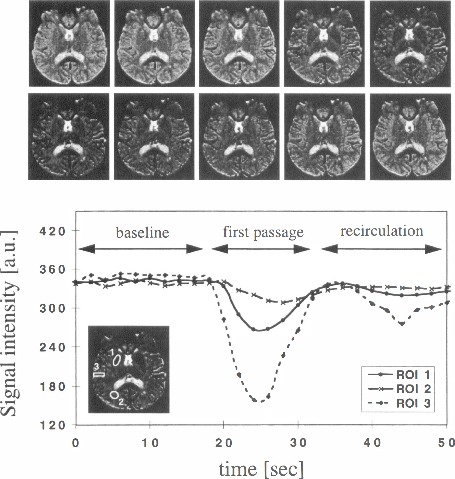
Basic theory
The model used for perfusion quantification is based on the principles of tracer kinetics for nondiffusable tracers (Zierler, 1962; Zierler, 1965; Axel, 1980) and relies on the assumption that in the presence of an intact BBB, the contrast material remains intravascular.
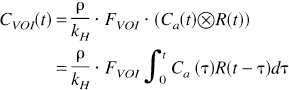
Considering a bolus of contrast material injected into the tissue, the concentration CVOI(t) of tracer within a given volume of interest (VOI) at a later time t can be defined in terms of three functions (Axel, 1995; Østergaard et al., 1996b):
Transport function, h(t): Probability density function of transit time t through the VOI following an ideal instantaneous unit bolus injection. This reflects the distribution of transit times through the voxel, which is dependent on the vascular structure and flow.
Residue function, R(t): Fraction of tracer still present in the VOI at time t following an ideal instantaneous unit bolus injection. By definition,
Arterial input function (AIF), Ca(t): Concentration of contrast agent in the feeding vessel to the VOI at time t.
With these definitions, the concentration CVOI(t) can be written in terms of a convolution of the residue function and the arterial input function (Østergaard et al., 1996b):
Therefore, to calculate CBF, Eq. 1 must be deconvolved (see later) to isolate FVOI · R(t) and the flow obtained from its value at time t = 0 (initial point of the deconvolved response curve). However, in practice, the measured AIF may be affected by both a delay and dispersion between the artery where it was estimated and the more peripheral tissue (VOI). As described by Østergaard et al. (1996b), these effects introduce spreading of the deconvolved curve, and instead of the initial point (which would underestimate the flow) the maximum of the curve should be used. To minimize these effects, the AIF should be measured as close as possible to the VOI.
Another important physiologic parameter that can be obtained by using DSC-MRI is CBV. For an intact BBB, CBV is proportional to the normalized total amount of tracer,
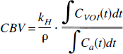
The normalization to the AIF accounts for the fact that, independent of the CBV, if more tracer is injected, a greater concentration will reach the VOI. Notice that because the arterial input to an organ is ultimately derived from a common source, relative CBV (relCBV) can be measured without any knowledge of the AIF (Rosen et al., 1990). This is one reason for the popular use of regional CBV maps in early DSC studies.
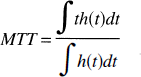
The third physiologic parameter, MTT, is the average time required for any given particle of tracer to pass through the tissue after an ideal bolus injection. By using the definition of the transport function, MTT can be written as the ratio of the first moment of the transport function to its zeroth moment 0:
In the classic outflow experiment (where the concentration in the venous output, Cout(t), is measured), the MTT can be calculated from the first moment of the tracer concentration (Axel, 1995). However, as pointed out by Weisskoff et al. (1993), this MTT is distinct from the first moment of CVOI(t). The latter depends on the topologic makeup of the vasculature. Therefore, calculation of MTT cannot be performed without first solving Eq. 1.
Once CBF and CBV are known, MTT also can be calculated directly by using the central volume theorem (Stewart, 1894; Meier and Zierler, 1954):

Conversely, some studies have used the central volume theorem to estimate a “perfusion index” (“CBFi”) from the ratio of the CBV to the first moment of concentration–time curve. However, apart from the previously mentioned dependency on the underlying vascular structure, this “perfusion index” is influenced by the shape of the bolus, since the first moment contains contributions from both the MTT and the first moment of the AIF (Axel, 1995). The shorter the MTT, the more important this extra contribution becomes, and a simple linear relation between FVOI and “CBFi” is not expected, particularly at high flow values (Wittlich et al., 1995). In addition to the assumptions of an intact BBB and stable flow during the measurement, some extra assumptions are necessary for the model described earlier to be valid: (1) that the contrast agent used is really a tracer, that is, it has no effect on the CBF (Doerfler et al., 1997) and has negligible volume itself; (2) that recirculation of the tracer is negligible (see later); (3) that the change in T1 relaxation is negligible; and (4) that dispersal and delay of the bolus as it reaches the VOI are not significant. This last assumption is likely to be invalid during ischemia and, as discussed later, can produce an underestimate of the calculated perfusion.
Quantification issues
One of the fundamental points regarding the use of the model described earlier is the need to convert changes in regional MR signal intensity to contrast agent concentration time curves; that is, since MRI is not able to directly measure the tracer concentration, it must be measured indirectly through its effect on signal intensity. It has been shown, both empirically (Villringer et al., 1988; Rosen et al., 1990; Hedehus et al., 1997) and using Monte Carlo simulations (Fisel et al., 1991; Weisskoff et al., 1994; Boxerman et al., 1995; Kennan et al., 1994), that the concentration of the tracer in the VOI is approximately proportional to the change observed in the relaxation rate R2 (= I/T2) or R2* in normally perfused tissue. By assuming a single exponential relation, the change in relaxation rate (ΔR2) can be obtained from the change in signal intensity from the baseline signal before contrast administration (S0).
Therefore, this technique allows, in principle, the quantification of regional CBF, CBV, and MTT. However, because of practical and theoretical difficulties, quantification using more simplistic approaches has been used commonly. There are three main different approaches to the quantification of data obtained using DSC-MRI: (1) quantification of absolute CBF; (2) quantification of relative CBF (relCBF); and (3) quantification using summary parameters, such as time-to-peak (TTP), bolus arrival time (BAT), maximum peak (MP), full width at half maximum, peak area, first moment of the peak (C(1)VOI), and parameters defined from the coefficients of the Gamma-variate function (see later).
The first two approaches require the deconvolution of the AIF and, therefore, are technically demanding. An accurate characterization of the AIF also is required (see later). The use of summary parameters, on the other hand, does not require the deconvolution of the measured signal and has been widely used, both in animal and human studies because of its much simpler and less time-consuming processing (see Applications of Perfusion Imaging Using MR Contrast Agents). However, it has disadvantages compared with the other approaches, since there is no simple relation between the summary parameters and CBF. They also depend on other factors such as CBV, MTT, bolus volume and shape, injection rate, and cardiac output. This makes the interpretation of summary parameter maps less straightforward, and in general, it depends on assumptions about the underlying vascular structure (Weisskoff et al., 1993; Gobbel et al., 1991). Furthermore, accurate comparison between subjects, or repeated measurements in follow-up studies, is not possible. However, when no information about the AIF is accessible, summary parameters are the only quantitative option and, in many cases, they can be useful in helping to distinguish between various pathologic and physiologic situations.
Deconvolution methods. Several methods to deconvolve Eq. 1 have been proposed. Østergaard et al. (1996b) have compared the performance of some of them, both using Monte Carlo simulations and experimental data. They analyzed two main categories of deconvolution approaches: model-dependent (Jacquez, 1972) and model-independent techniques (Gobbel and Fike, 1994; Rempp et al., 1994). In the first, an empirical analytical expression is chosen to describe the tracer vascular retention, that is, a specific analytical expression for R(t) is assumed. The most common model is to consider the vascular bed as one single, well-mixed compartment, and therefore R(t) = exp(–t/MTT) (Bassingthwaighte and Goresky, 1984; Lassen et al., 1984). In the second, the model-independent approach, both CBF and R(t) are determined by nonparametric deconvolution, that is, the residue function is also treated as an unknown variable. This approach can be subdivided in two categories. In the transform approach, the convolution theorem of the Fourier transform is used to deconvolve Eq. 1:
The results obtained by Østergaad et al. (1996b) indicate that model-dependent approaches predict correct absolute CBF values only if the actual residue function is sufficiently described by the assumed model. It also can yield a reasonable estimate of relative flow when the shape of R(t) is relatively uniform across the brain. However, this is not likely to be the case in pathologic tissue or in tissue with altered hemodynamics. In the case of the Fourier transform approach, the estimate of CBF was shown to be biased by the CBV, producing underestimates in cases of high flow and short MTT (relative to the sampling rate). The nonparametric deconvolution using regularization was found to give accurate flow values over a wide range, although it also showed some dependency on the vascular volume. Finally, their results showed that the singular value decomposition technique gave, in general, good accuracy, independent of the underlying vascular structure, R(t), and volume, CBV, even for a signal-to-noise ratio (SNR) typical of EPI.
Other deconvolution approaches have been adopted, such as deconvolution using orthogonal polynomials (Schreiber et al., 1998 and references therein), where the AIF is approximated by a subset of an orthogonal function system, and Eq. 1 is solved analytically, or the use of a maximum likelihood method, where the equation is solved iteratively (Vonken et al., 1998). However, a complete description of deconvolution methods is beyond the scope of this review.
Studies of flow quantification using continuous and pulsed arterial spin labeling and dynamic susceptibility contrast MRI techniques
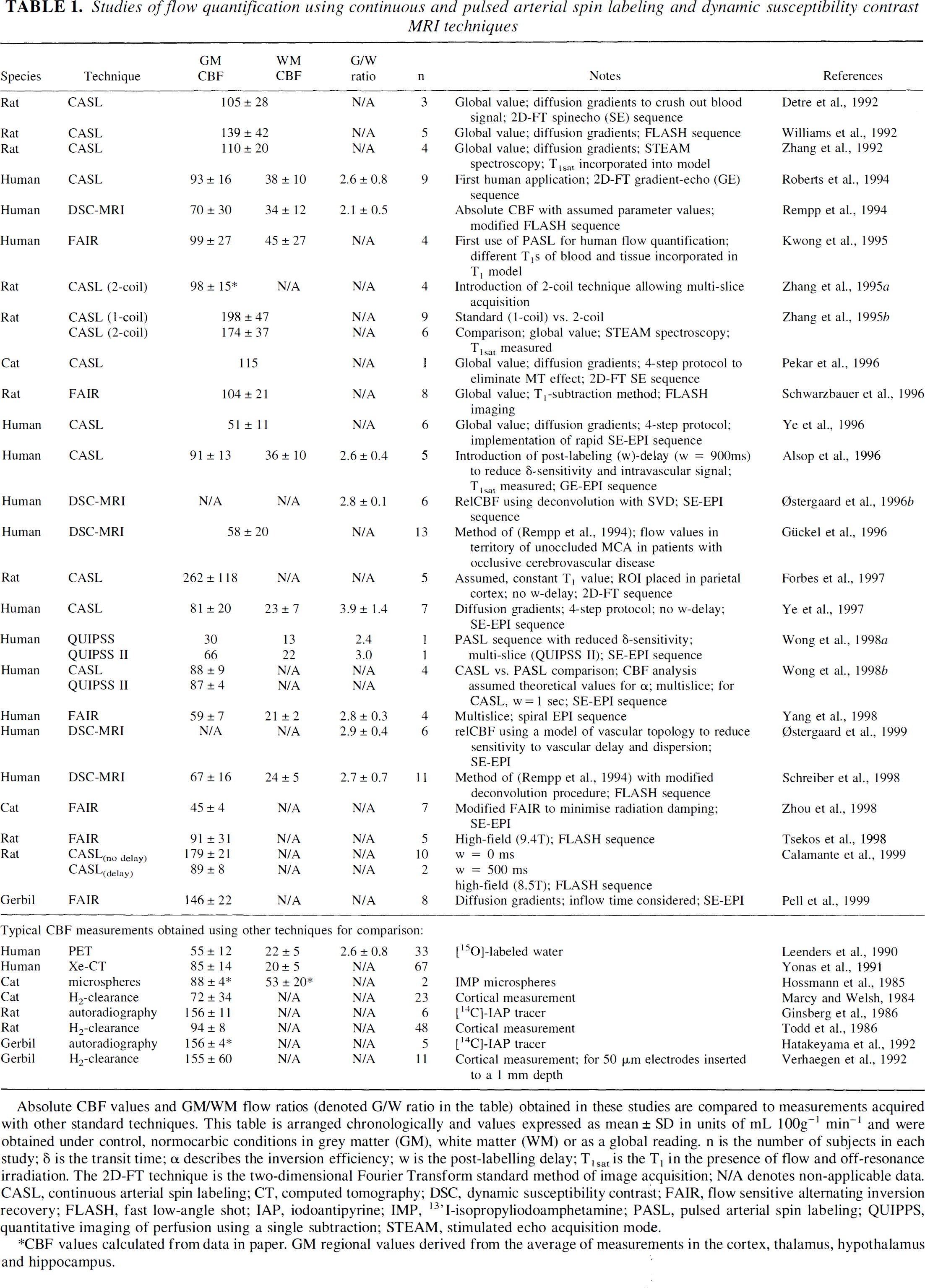
Absolute CBF values and GM/WM flow ratios (denoted G/W ratio in the table) obtained in these studies are compared to measurements acquired with other standard techniques. This table is arranged chronologically and values expressed as mean ± SD in units of mL 100g−1 min−1 and were obtained under control, normocarbic conditions in grey matter (GM), white matter (WM) or as a global reading. n is the number of subjects in each study; δ is the transit time; α describes the inversion efficiency; w is the post-labelling delay; T1sat is the T1 in the presence of flow and off-resonance irradiation. The 2D-FT technique is the two-dimensional Fourier Transform standard method of image acquisition; N/A denotes non-applicable data. CASL, continuous arterial spin labeling; CT, computed tomography; DSC, dynamic susceptibility contrast; FAIR, flow sensitive alternating inversion recovery; FLASH, fast low-angle shot; IAP, iodoantipyrine; IMP, 13'I-isopropyliodoamphetamine; PASL, pulsed arterial spin labeling; QUIPPS, quantitative imaging of perfusion using a single subtraction; STEAM, stimulated echo acquisition mod
CBF values calculated from data in paper. GM regional values derived from the average of measurements in the cortex, thalamus, hypothalamus and hippocampus.
An alternative approach for the calculation of absolute CBF values involves cross-calibration with another technique (Østergaard et al., 1998a, b ; Wittlich et al., 1995). In one of these studies, CBF measurements were performed using DSC-MRI and PET in the same animals (normocapnic and hypercapnic pigs) (Østergaard et al., 1998b). By comparing average flow rates through all regions, a common empirical conversion factor (to absolute flow units) was obtained for DSC measurements. Recently, this cross-calibration also was performed on normal human subjects (Østergaard et al., 1998a). However, the validity of the same conversion factor in patients with altered hemodynamics and for different tissue types remains to be shown. A similar approach using DSC-MRI and autoradiography was used to calculate absolute CBF in rats during middle cerebral artery occlusion (MCAO) (Wittlich et al., 1995). However, in this study, the AIF was not measured, and the MTT was approximated by C(1)VOI.
Notice that since the same proportionality constants are assumed for the normalization of CBF and CBV, the ratio of CBV/CBF will be an absolute measure of MTT (Østergaard et al., 1996b).
Recirculation or leakage of the tracer. The model previously described is only for the first pass of the tracer. However, the measured CVOI(t) can include contributions from recirculation (which can be recognized as a second, smaller concentration peak or an incomplete return to baseline after the first pass; Fig. 1). Therefore, these contributions must be eliminated before any perfusion calculation. This can be achieved, either by considering the curve only until the appearance of the recirculation, or by fitting a portion of the concentration time curve to an assumed bolus shape function, typically a gamma-variate function, Γ (Starmer and Clark, 1970; Berninger et al., 1981).
In a Monte Carlo study of the CBV dependency on the SNR of the base images, Boxerman et al. (1997) showed that numerical integration and Γ-fitting gave similar results for DSC images with SNR greater than 20 to 30. However, for lower SNR, the variability introduced by the covarying parameters in the Γ-fitting yielded CBV maps with decreased SNR. Although similar conclusions are expected to be valid for CBF, further simulations are needed to extend these findings.
The presence of a. damaged BBB results in leakage of the tracer to the extracellular space. This leads to a decrease in the susceptibility effects and to an increase in T1 relaxation rate, which opposes the signal losses from T2 (usually seen as a positive slope after the return of the peak to baseline). These effects can be minimized with a proper choice of pulse sequence parameters, and, in cases of a moderate BBB disruption, a technique to correct for T1 enhancement in CBV maps has been proposed (Weisskoff et al., 1994). An alternative in cases of a disrupted BBB is the use of a dysprosium-based contrast agent (Dy-type) instead of a gadolinium-type (Gd-type) (Kucharczyk et al., 1993; Lev et al., 1997). Because of its much smaller T1 enhancement (ΔR1(Dy) ≈ ΔR1(Gd)/40 (Villringer et al., 1988; Moseley et al., 1991)), this contrast agent should give more accurate perfusion calculations. Also notice that when the BBB is damaged, contrast agents can be used to extract information about BBB permeability by modeling the leakage of the tracer out of the intravascular space. This has been an area of great interest in the study of brain tumors and multiple sclerosis, but its description is outside the scope of this review (see Tofts, 1997 for a recent review).
Measurement of the arterial input function. The AIF depends not only on the shape of the injected bolus but also on the cardiac output, the vascular geometry, and the cerebral vascular resistance (Mottet et al., 1997). The AIF can be estimated directly by measuring the signal loss in a region of interest positioned on (or around) a feeding cerebral artery, such as the carotid artery or the middle cerebral artery (MCA) (Porkka et al., 1991; Rosen et al., 1991b; Perman et al., 1992). The signal in such a region would show an early, large increase in R2 after contrast injection. The AIF generated in this way is commonly used, and in preliminary data, it has been shown to be proportional to measurements obtained invasively by arterial blood sampling in animals (Porkka et al., 1991; Rosen et al., 1991b). However, a full study to confirm these findings remains to be performed. Furthermore, because of partial volume effects with surrounding tissue, the AIF may be underestimated, thereby overestimating the CBF.
For a given contrast agent, higher sensitivity with the DSC technique can be obtained by increasing the injected dose or by using a longer TE. However, because of the greater concentration of the tracer in the arterial supply than in the VOI, a larger arterial signal drop is observed. If the signal falls below the background noise level, the AIF will be underestimated, introducing errors to the CBF quantification. To reduce this source of error, two different echo times can be used, with a shorter TE for the determination of the AIF (Perman et al., 1992; Rempp et al., 1994; Schreiber et al., 1998). Another possibility is to use only those measurements that fall above the background noise (Østergaard et al., 1998b; Ellinger et al., 1998).
Sequence type (gradient-echo versus spin-echo)
Dynamic susceptibility contrast MRI can be used either with spin-echo (SE) or gradient-echo (GE) imaging, since the passage of the bolus affects both T2 and T2*. Because of the larger effect observed using GE, most of the original studies used this type of sequence to follow the passage of the tracer through the brain. However, Monte Carlo simulations have shown that the susceptibility contrast in GE images arises from both large and small vessels, whereas in SE images it is dominated by small, capillary-sized vessels (Weisskoff et al., 1994; Boxerman et al., 1995; Kennan et al., 1994). Therefore, more studies are being performed using SE techniques, reflecting more microvascular perfusion. Furthermore, SE images offer improved image quality, particularly in regions such as the temporal lobes and the frontal sinus. However, notice that the CBV determined in this way is not the total CBV (even after accounting for the hematocrit concentration) but just the microvascular CBV (Boxerman et al., 1995; Østergaard et al., 1998b).
APPLICATIONS OF PERFUSION IMAGING USING MR CONTRAST AGENTS
Because of the technical difficulties and the assumptions involved in the quantification of absolute CBF, most of the applications of DCS-MRI have used summary parameters. Table 1 summarizes the studies of flow quantification.
Studies of experimental animal models
Cerebral ischemia. One of the first applications of the DSC technique was in the study of cerebral ischemia in experimental animal models. Unlike conventional MRI (T1, T2, and proton density), which is insensitive to acute ischemia, diffusion-weighted imaging (DWI) and DSC-MRI were shown to detect stroke within minutes of the event. Thus, much of the interest in the earlier studies was on the acute identification of ischemic regions (Moseley et al., 1990; Maeda et al., 1993; Wendland et al., 1991; Finelli et al., 1992; Kucharczyk et al., 1991). However, since the area with a perfusion deficit was found to be larger than the area depicted by DWI, the emphasis moved toward the use of DSC-MRI to complement and help in the interpretation of the changes observed using conventional MRI and DWI, with the ultimate aim of identifying and characterizing the ischemic penumbra (Astrup et al., 1981).
Within this context, combined diffusion and DSC-MRI summary parameters were used to identify a severe ischemic central area surrounded by a more moderately affected peripheral area in transient MCAO studies in rats (Muller et al., 1995a), as well as in permanent MCAO studies in cats (Moseley et al., 1990; Moseley et al., 1993) and rats (Pierce et al., 1997; Quast et al., 1993; Dijkhuizen et al., 1997). Pierce et al. (1997) showed that the apparent diffusion coefficient (ADC) was linearly correlated with MP signal in the periphery and suggested that their combined study could be useful for the quantitative assessment of the variable flow gradients in focal ischemia, including potentially critical areas at risk in the ischemic periphery (Fig. 2).
(A) Perfusion-sensitive magnetic resonance (MR) images of the first-pass transit of gadodiamide in rat focal ischemia. Gadodiamide transit induces a transient drop in MR signal intensity. Focal ischemia is evident as regions that show no signal change. Imaging speed is one image per second using fast low-angle shot imaging. 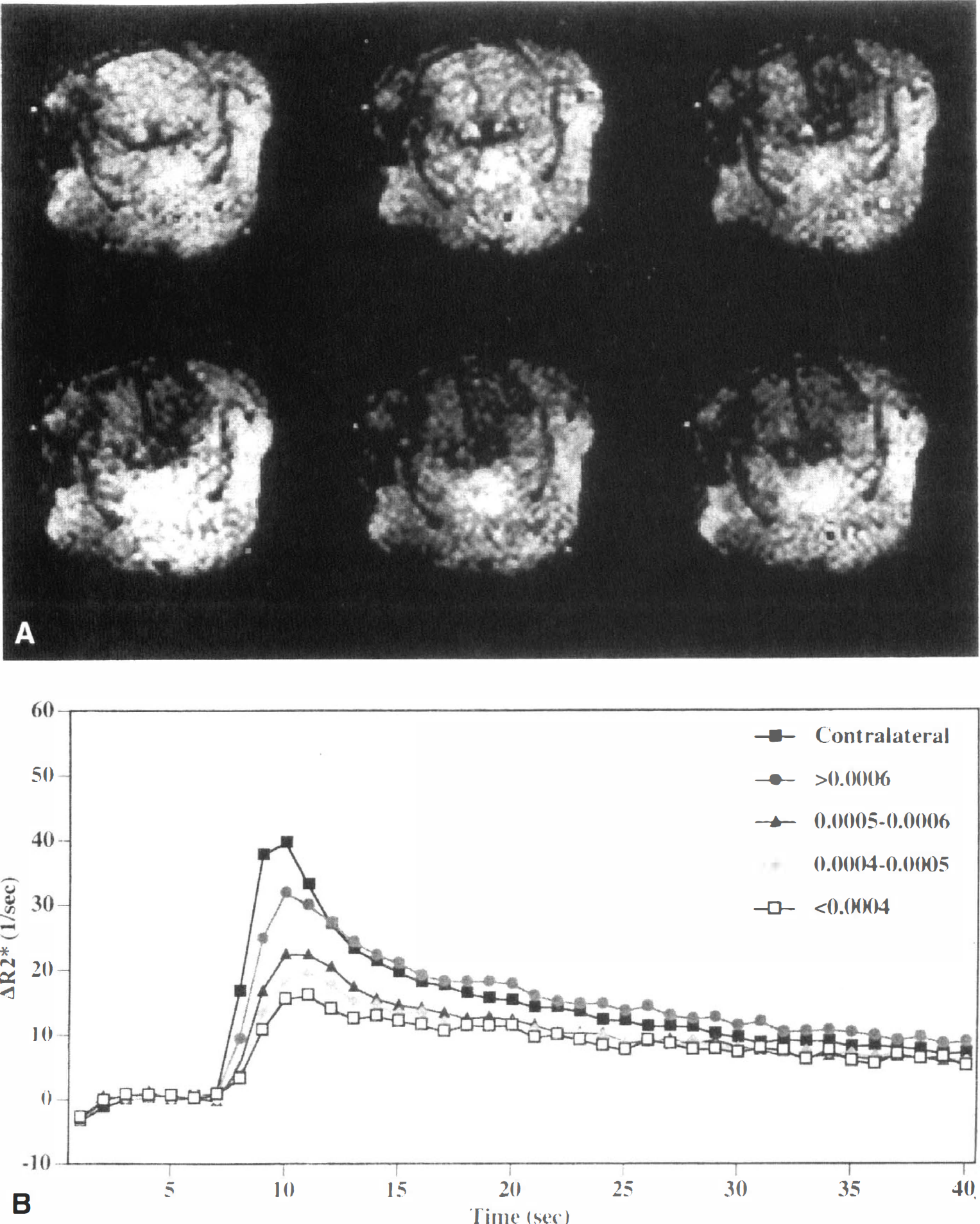
A similar approach was used to identify different levels of ischemia in a cat model of partial MCAO (Fig. 3). The combination of high-speed ADC measurements and MP signal allowed the differentiation of mild (no change in ADC and slight reduction in the MP), moderate (slight reduction in ADC and reduced MP), and severe cerebral hypoperfusion (marked drop in ADC and almost complete absence of contrast agent passage) (Roberts et al., 1993; Roberts et al., 1996). Similar results were obtained recently using ADC, MP, BAT, and high magnetic field T2 mapping in models of hypoperfusion and focal cerebral ischemia in the rat (Grohn et al., 1998).
(A) Time course of ΔR2* in a cat model of mild ischemic injury with no sign of injury on triphenyltetrazolium chloride (TTC) staining and no apparent hyperintensity on diffusion-weighted imaging (DWI). A drop in the peak ΔR2* effect of −20% in the ischemic parietal cortex and a delay of 4 to 6 seconds relative to the contralateral normal cortex are typical. Numerical fits to the gamma-variate function, also shown, allow a better estimate of the peak ΔR2* effect and eliminate effects of recirculation of contrast agent in the asymptotic tail of the ΔR2* curves. 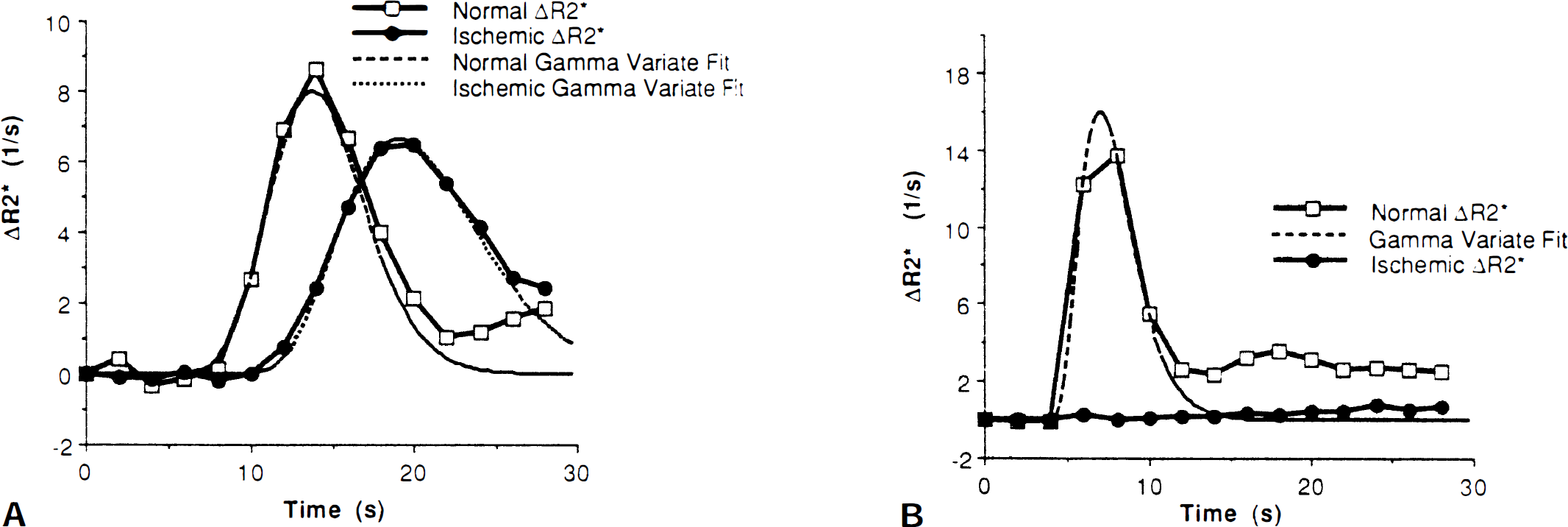
The DSC summary parameters also were used to study the reperfusion state in transient MCAO in the cat (Kucharczyk et al., 1993), distinguishing between successful and failed reperfusion and identifying delayed reperfusion injury. Recently, in a study of delayed damage in a model of temporary hypoxia–ischemia in the rat, it was shown that ADC alone was a bad predictor of long-term outcome (Dijkhuizen et al., 1998). Measurements of ADC, T2-weighted imaging, DSC summary parameters (MP, TTP, and peak area), laser-Doppler flowmetry, and histologic study were used to show different regional response to reperfusion and an associated tissue-specific sensitivity to delayed damage.
In a study of transient focal ischemia in cats (Caramia et al., 1998), DSC summary parameters were used to identify the hemodynamic spatial heterogeneity in response to ischemia and reperfusion. In particular, a peripheral area of increased vascular transit time (VTT = TTP – BAT) was observed, which was interpreted as a mismatch between CBF and CBV. This area had a different response to reperfusion compared with the core region.
Another application, where DSC summary parameters were used, is to the determination of the relation between apoptosis and perfusion deficits during transient cerebral ischemia in cats. Vexler et al. (1997) showed that a significantly higher number of apoptotic cells were observed in areas that experienced 2.5 hours of severe perfusion deficit (regardless of the state after reperfusion) compared with the number in areas with reduced but maintained perfusion. These results suggest that the apoptotic process is induced in the ischemic core and contributes in the degeneration of neurons associated with transient ischemia.
Cortical spreading depression. The DSC summary parameters (relCBV and TTP) also have been used in the study of cortical spreading depression. By following the ADC changes in ischemia-induced spreading depression, Rother et al. (1996a), (b) showed that these transient ADC changes originated in the border of the core region, where there was a moderate perfusion deficit (increased bolus transit time), and that the variation in the ADC recovery time in the ischemic periphery reflected the severity of the tissue perfusion deficit.
De Crespigny et al. (1998) studied the changes in relCBV and ADC during spreading depression in rats, although not using DSC techniques. In this study, steady-state CBV measurements using a blood pool contrast agent were performed simultaneously with high-speed ADC mapping. They found transient regional hypoperfusion after the ADC changes with a variable delay (average value of ~16 seconds), thought to be a consequence of the elevated energy requirements during the repolarization after spreading depression.
Therapeutic evaluation. The combined used of DSC-MRI and DWI provides an excellent tool to investigate the effect of new therapeutic interventions in models of embolic stroke in animals. Reith et al. (1996) have assessed the effects of thrombolytic therapy using recombinant tissue plasminogen activator (rt-PA) in a rat model, whereas more recently, Yenari et al. (1997) have examined the combined effect of rt-PA and direct antithrombin therapy using hirulog in rabbits. Furthermore, the effect of rt-PA has been studied in a model of cerebral venous thrombosis (Röther et al., 1996d). Bolus tracking techniques also have been used to evaluate the cerebroprotective effects of noncompetitive N-methyl-
Clinical applications
Cerebrovascular diseases. Because of the insensitivity of conventional MRI for the detection of acute stroke and the lack of a definite treatment in the early 1990s, few studies of cerebral ischemia were performed during the hyperacute phase (first few hours), and, therefore, the affected area was already visible on T2-weighted images. In these studies, DSC-MRI was mainly used to evaluate the perfusion state of the affected region and provide extra information, which was not available from conventional MRI (Edelman et al., 1990; Warach et al., 1992). Furthermore, since EPI capabilities were not available in many centres, the initial studies were restricted to single-slice acquisitions using fast GE sequences. In some studies during the hyperacute phase, the selected slice did not include the ischemic region, and false-negative results were obtained (Warach et al., 1992; Röther et al., 1996c). With the advent of thrombolytic therapy and the need for an early assessment of the affected area, the emphasis on DSC studies changed toward hyperacute diagnosis, identification of tissue at risk, and prediction of neurologic outcome.
Many studies address the mismatch between the region of perfusion disturbance, the area with reduced diffusion, and the possible relation with tissue at risk of infarction (Fig. 4) (Sorensen et al., 1996, 1997; Østergaard et al., 1996a; Rordorf et al., 1998; Tong et al., 1998; Schwamm et al., 1998; Baird et al., 1997; Barber et al., 1998). In studies during the hyperacute phase using magnetic resonance angiography, ADC, and relative CBV (Sorensen et al., 1996; Rordorf et al., 1998), it was possible to classify the MCA stroke into different clinical and pathophysiologic subtypes. Group 1 (patients with M1 occlusion) presented a mismatch between the extent of early infarction (as defined by DWI) and the extent of early ischemia (as defined by DSC-MRI), and they usually showed a progression of infarction into the larger region of abnormal perfusion. Group 2 (patients with open M1 on magnetic resonance angiography and stroke from occlusion of a distal branch) presented a matched diffusion/perfusion abnormality and were found to have maximal extent of regional injury on their initial study (Fig. 5). As suggested by the authors, this classification may help to the selection of patients who could benefit from thrombolytic and neuroprotective therapies.
Images of a 53-year-old man 3 hours after acute onset of left hemi-paresis. (A) A 62-year-old man had sudden onset of dense right hemiplegia 7 hours before his MRI scan. The T2 sequence shows only a subtle increase in signal in a gyral pattern, whereas the DWI map shows an ischemic injury (arrow) located mostly in the insular and periinsular cortex. The CBV map demonstrates a perfusion abnormality much larger than the DWI abnormality. Magnetic resonance angiography (MRA) demonstrates a left MCA occlusion (arrow). In the follow-up MRI, the stroke has expanded beyond the initial area of perfusion abnormality. 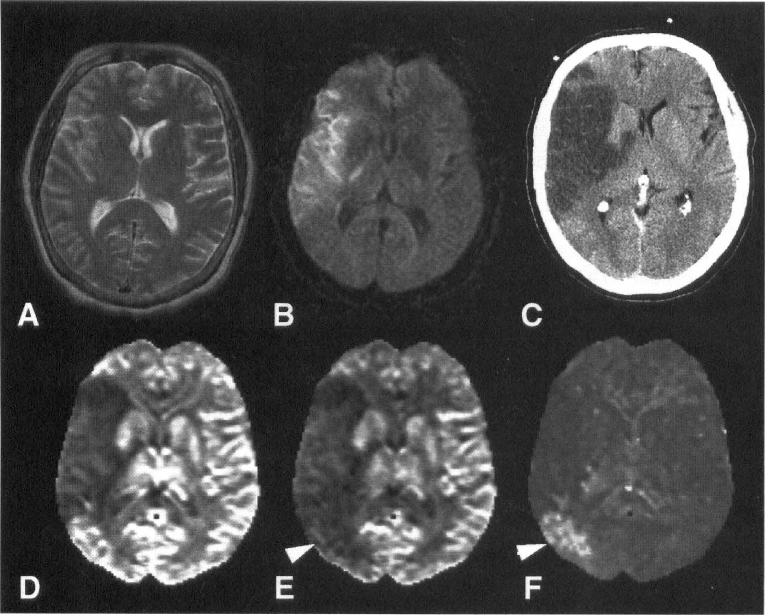
In a different approach to the identification of tissue at risk, some studies examine the concentration–time curves in the different areas (Röther et al., 1996c; Tsuchida et al., 1997; Reith et al., 1997). Röther et al. (1996c) analyzed DSC summary parameters during the first 6 hours after symptoms onset. Three different patterns for the passage of the tracer, depending on the perfusion status of the tissue, were identified: in the center of the lesion, a complete loss of the bolus passage (pattern 1) was associated with the infarct core; a delayed bolus, with reduced peak and increased width (pattern 2) was taken to represent the potentially salvageable tissue; and, finally, a minimal bolus delay with a slightly reduced peak (pattern 3) was observed only in follow-up studies in regions that showed a marked recovery.
In a preliminary analysis of patients with severe clinical deficits, Warach et al. (1996) found that the combined use of DWI and DSC-MRI (relCBV) was highly accurate in predicting clinical outcome by identifying the patients who would improve. The advantage of combined DWI/DSC-MRI analysis compared with conventional MRI was found to be more important in the subgroup of patients studied during the first 6 hours. In a study on the correlation between lesion volume (measured by DWI or DSC-MRI) and neurologic deficit (quantified using the National Institutes of Health Stroke Scale), Tong et al. (1998) report a significant correlation between initial lesion size (measured within 6.5 hours of symptom onset) and the score on the National Institutes of Health Stroke Scale for both DWI and DSC-MRI volumes. In a similar study, Barber et al. (1998) found a high correlation between DSC-MRI lesion volumes (using C(1)) and acute neurologic state (assessed by the Canadian Neurological Scale), clinical outcome (Canadian Neurological Scale, Barthel Index, and Rankin Scale), and final infarct volume (T2-weighted imaging). However, the correlation of acute DWI lesion volumes was not as robust. These authors suggest that the difference from the previous study may result from the different clinical scales used or to a different proportion of patients with perfusion deficits larger than the region of reduced diffusion (which are more likely to have lesion enlargement). This highlights the need to study numerous patients before these correlations can be established and emphasizes the danger of extending particular findings to different patient populations.
Although further studies are needed, it is expected that a combined analysis using DWI and DSC-MRI (together with magnetic resonance angiography and conventional MRI) could be used to identify patients who might benefit from various treatment modalities and those who can avoid the potential risks associated with thrombolysis and neuroprotective agents. Furthermore, the duration of a therapeutic window may need to be defined for individual patients, depending on the physiologic state of the tissue, instead of being defined only by the time from symptom onset (Baron et al., 1995; Fisher, 1997). This is supported by recent data that show expansion of ischemic lesions several hours, and even days, after the acute insult (Baird et al., 1997; Schwamm et al., 1998). Therefore, DWI and DSC-MRI could improve patient selection, guide stroke therapy, and, therefore, improve the evaluation of new therapeutic strategies.
In patients with unilateral symptomatic internal carotid artery (ICA) occlusion, DSC-MRI also was used to assess perfusion deficits (Gückel et al., 1994; Nighoghossian et al., 1996; Kluytmans et al., 1998). All of these studies show changes in various summary parameters, suggesting an impairment of perfusion reserve in the ipsilateral side. Furthermore, these hemodynamic changes occurred mainly in white matter regions (Kluytmans et al., 1998), which is consistent with its higher vulnerability in patients with ICA occlusion.
The DSC summary parameters have been used to evaluate the perfusion characteristics in children with homozygous sickle cell anemia (both with and without clinical evidence of cerebrovascular disease) (Tzika et al., 1993), in patients with moyamoya disease (Tzika et al., 1997; Tsuchiya et al., 1998), and, in conjunction with the blood oxygenation level–dependent (BOLD) contrast technique, to study functional brain activation in patients with chronic cortical stroke (Sorensen et al., 1995).
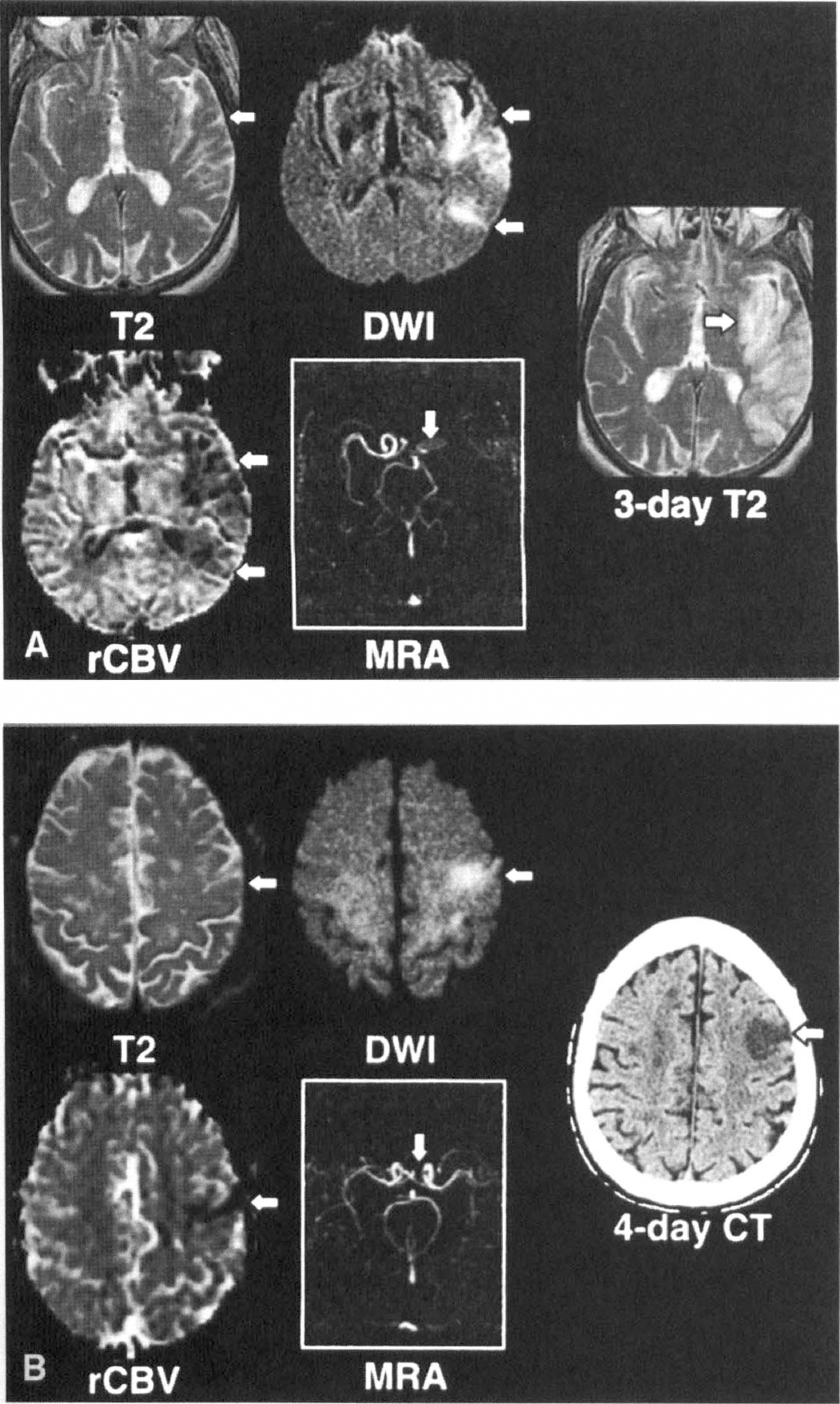
Notice that because of its dynamic characteristic, DSC-MRI can provide perfusion related information not available from PET or single photon emission computed tomography (SPECT) studies. For example, in a study 5.5 hours after stroke onset, Sorensen et al. (1997) showed that despite the apparently normal shape and area of the bolus (probably indicative of unaffected CBV and CBF), there was only a delayed bolus arrival to the ischemic tissue, consistent with slow collateral flow through feeding arteries. Similar results also were obtained in an area adjacent to a chronic stroke (Fig. 6) (Sorensen et al., 1995).
Evaluation of stroke with perfusion imaging. 
Cerebrovascular reactivity. Acetazolamide (ACZ) is a potent vasodilatory agent that is being increasingly used clinically to test the vascular reserve in cases of large artery cerebrovascular disease. Dynamic susceptibility contrast MRI provides a means to assess cerebrovascular reactivity by performing two bolus injections of contrast agent: one before (to obtain a baseline measurement), and the other after the ACZ administration. Several studies address the ability of DSC-MRI to measure CBV changes in normal volunteers (Levin et al., 1995; Petrella et al., 1997; Berthezene et al., 1998) and the age dependency of this vasodilatory response (Petrella et al., 1998).
Two studies have been performed on the application of the ACZ stimulation test to patients with occlusive cerebrovascular disease (Gückel et al., 1996; Schreiber et al., 1998). These studies not only address the CBV response but also measure the effect on CBF and MTT. They are among the few studies where absolute quantification was performed. Gückel et al. (1996) assessed the cerebrovascular reserve capacity in patients with occlusion of the ICA or MCA. Regions of interest were chosen from the MCA territory but without including infarcted tissue. A statistically significant reduction in CBF response was found in the affected MCA territory, indicative of a severely compromised cerebrovascular reserve capacity. They also found a decoupling between CBV and CBF response to ACZ, suggesting that CBV alone is not a reliable indicator for the cerebrovascular reserve capacity. In a recent study, Schreiber et al. (1998) evaluate the response to ACZ in patients with occlusion or high-grade stenosis of the ICA, and a similar reduction in the cerebrovascular reserve capacity was found in peri-infarcted regions (Fig. 7). An interesting finding of this study was the correlation between the change in CBF and the baseline MTT value, which suggests that MTT baseline measurements could be used to assess cerebrovascular reserve capacity.
A patient with occlusion of the right internal carotid artery having transient ischemic attacks. 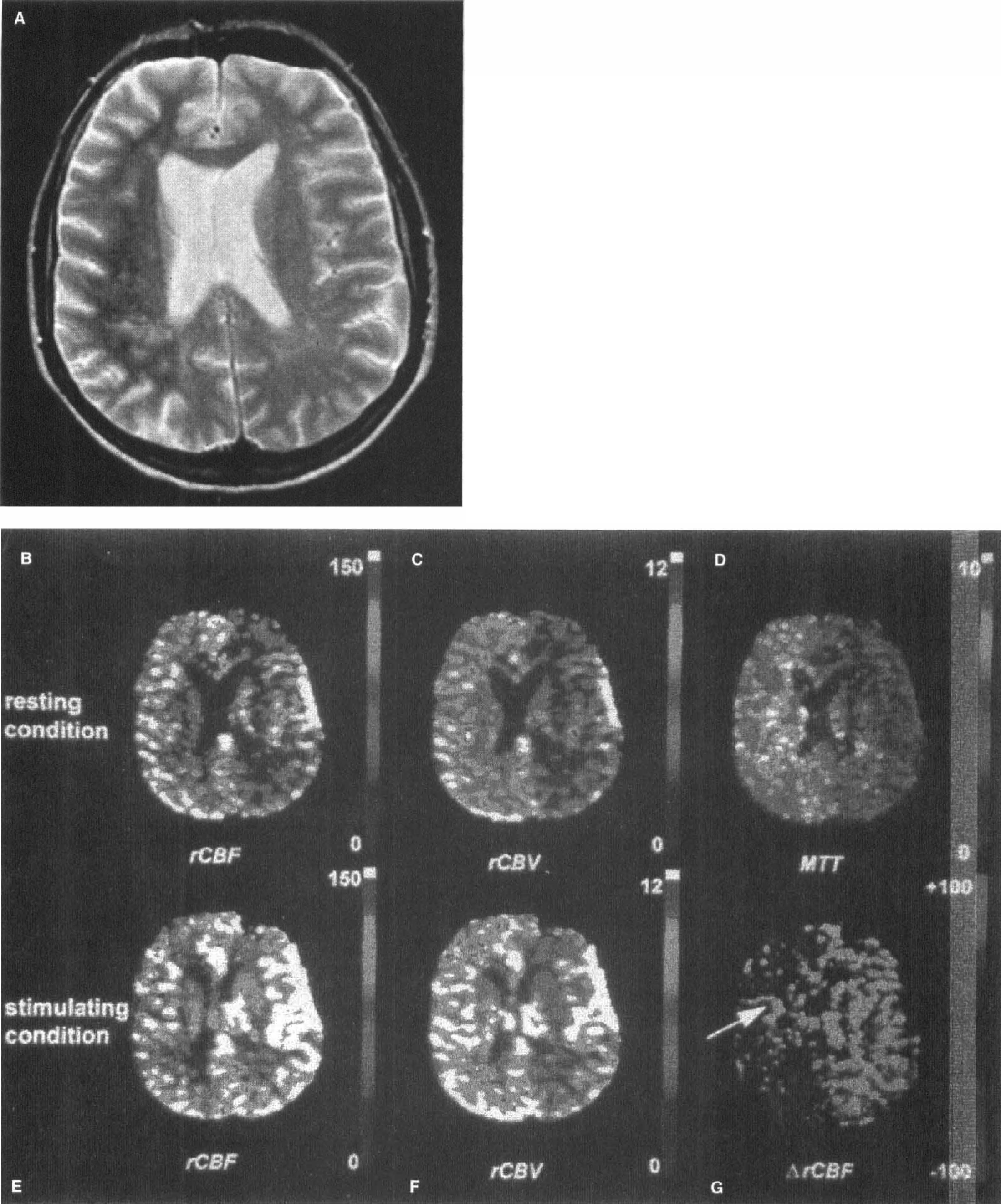
Notice that because the ACZ test requires multiple bolus injections, special care must be taken to avoid (or take account of) the effect of the residual contrast agent from the first injection on the second measurement (Runge et al., 1994; Levin et al., 1995; Levin et al., 1998).
Other applications. In a recent study, Cutrer et al. (1998) used DSC-MRI and DWI to study brain hemodynamics during spontaneous visual auras in patients with migraine headaches. Although the measurements of MTT, relCBF, and relCBV performed interictally were normal and symmetrical throughout the brain, a moderate focal reduction in all of these parameters was observed in the occipital lobe during visual aura. Interestingly, no significant change in water diffusion was observed, suggesting that the perfusion deficit was not severe or persistent enough to induce ADC changes.
Another clinical application for DSC-MRI is in the perfusion evaluation of chronic neurodegeneracive disorders such as Alzheimer's disease. Although no CBF evaluation has been performed, several studies have evaluated changes in relCBV and its correlation with PET (Gonzalez et al., 1995; Caramia et al., 1995), SPECT (Harris et al., 1998), and the scores on the MiniMental State Examination (Maas et al., 1997; Harris et al., 1996).
Dynamic susceptibility contrast MRI also has been used in other applications, in particular, to study changes in CBV, such as the increased CBV observed in patients who are positive for human immunodeficiency virus (Tracey et al., 1998), in schizophrenic patients (Cohen et al., 1995), and in patients with epilepsy (Warach et al., 1994), and to detect changes after cocaine administration both in humans (Kaufman et al., 1998) and animals (Li and Suojanen, 1995).
Brain tumors, because of their different blood flow and vascular patterns, also are good candidates for DSC studies. Most of these studies concentrate on the evaluation of CBV, although a few also address the CBF distribution (Fig. 8) or other DSC summary parameters (Østergaard et al., 1996a; Sorensen et al., 1997). A good correlation between CBV and tumor grade (Aronen et al., 1994; Rosen et al., 1991b) has been demonstrated. Cerebral blood volume mapping also has been used to differentiate recurrent tumor from radiation necrosis (Rosen et al., 1991a; Caramia et al., 1995; Sorensen et al., 1997), and to study the changes associated with radiotherapy in a group of patients with astrocytomas (Wenz et al., 1996). Tumor heterogeneity, not observed in conventional MRI (precontrast or postcontrast), has been shown on CBV maps (Rosen et al., 1991b; Caramia et al., 1995), and a recent comparative study using relative CBV, 201T1-SPECT and PET (Siegal et al., 1997), has shown the high sensitivity of DSC-MRI to small regional changes. In this study, a 63% and 55% rate of delayed detection compared with CBV was found using SPECT and PET, respectively, which resulted from the higher spatial resolution and sensitivity of CBV maps produced by DSC-MRI. However, notice that BBB breakdown may be present in many cases, resulting in extravascular leakage of the contrast agent. As mentioned in the section on perfusion imaging using MR contrast agents, this effect introduces errors in the measurement, unless one properly accounts for them.
(A) The relative cerebral blood volume (relCBV) map of a patient with a low-grade tumor in the right temporal lobe shows a moderately elevated CBV over an extensive area. 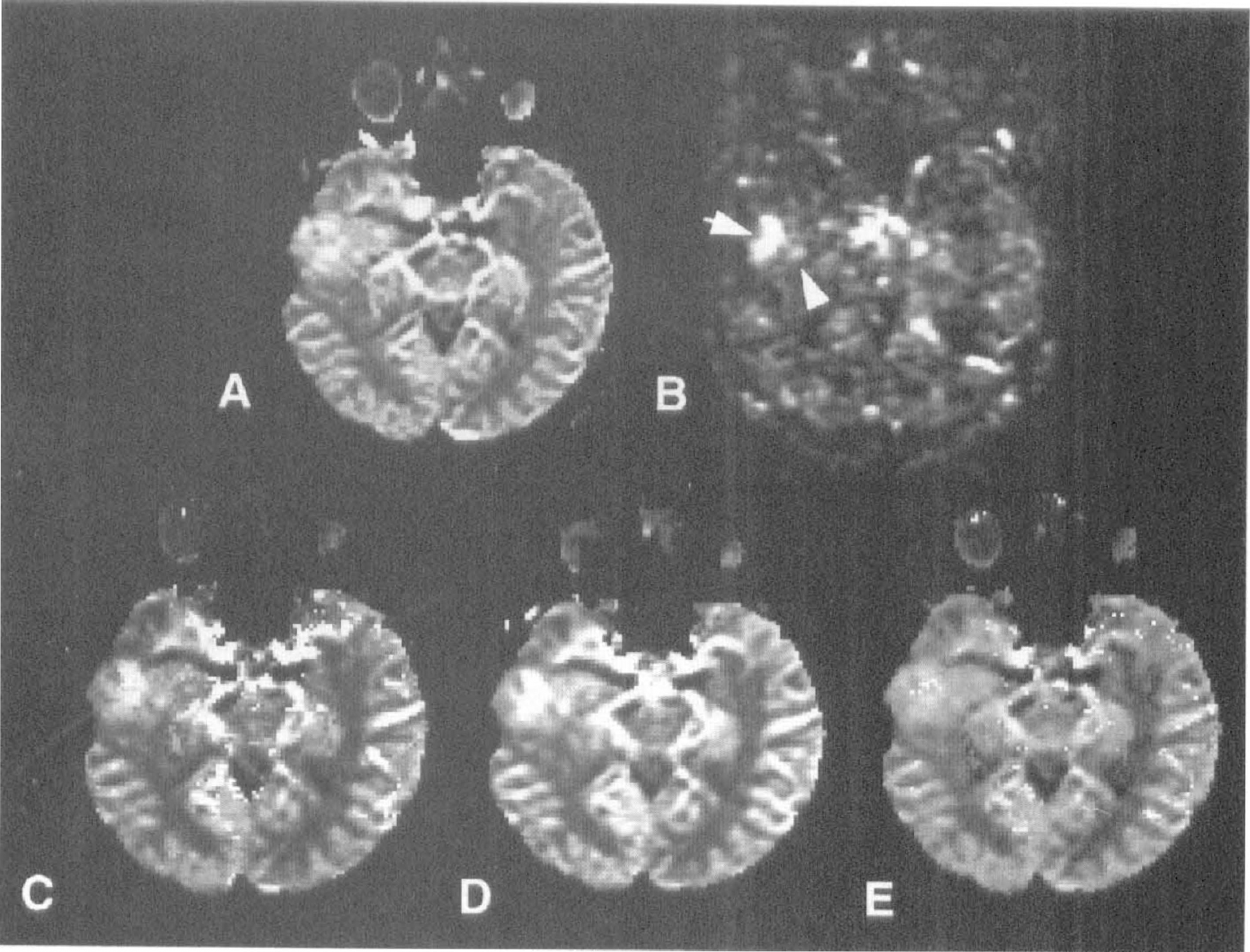
PERFUSION MRI USING SPIN LABELING OF ARTERIAL WATER
An MR image can be sensitized to the effect of inflowing blood spins if those spins are in a different magnetic state to that of the static tissue. The family of techniques known as ASL techniques uses this idea by magnetically labeling blood flowing into the slices of interest. Blood flowing into the imaging slice exchanges with tissue water, altering the tissue magnetization. A perfusion-weighted image can be generated by the subtraction of an image in which inflowing spins have been labeled from an image in which spin labeling has not been performed. Quantitative perfusion maps can be calculated if other parameters (such as tissue T1 and the efficiency of spin labeling, see later) also are measured. Since exogenous contrast agents are not required for these techniques, the perfusion measurement is completely noninvasive. Under the general heading of ASL, two distinct subgroups exist: continuous ASL and pulsed ASL. Despite sharing a similar basis, the two approaches have different advantages and limitations that affect their ability to quantify perfusion.
Continuous arterial spin labeling techniques
Basic theory. The first ASL technique, proposed by Detre et al. in 1992, is known as continuous arterial spin labeling (CASL). They suggest the use of a train of RF pulses to repeatedly saturate blood water spins flowing through the neck. The saturated (or “labeled”) spins flow into the brain and, assuming water is a freely diffusible tracer, exchange completely with brain tissue water, thus reducing the overall tissue magnetization. A steady state develops where the regional magnetization in the brain is directly related to CBF. This steady state can be derived from the Bloch equation for longitudinal relaxation when it is modified to include flow (Detre et al., 1992):
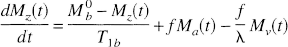
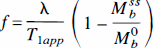
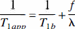
Equation 9 is the fundamental equation of ASL, describing how the apparent longitudinal relaxation time of brain tissue is affected by blood flow. By measuring T1app and the ratio of magnetization with and without arterial spin saturation, a value for flow can be calculated using Eq. 8.
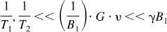
Soon after CASL was proposed, Williams et al. (1992) improved the technique by using adiabatic fast passage to label the arterial water spins. Making use of the adiabatic theorem (Abragam, 1961), the magnetization of a spin moving through a magnetic field gradient G at velocity v is inverted if a RF pulse is used to apply a constant B1 field perpendicular to the main field, and the following condition is satisfied:
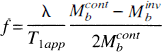
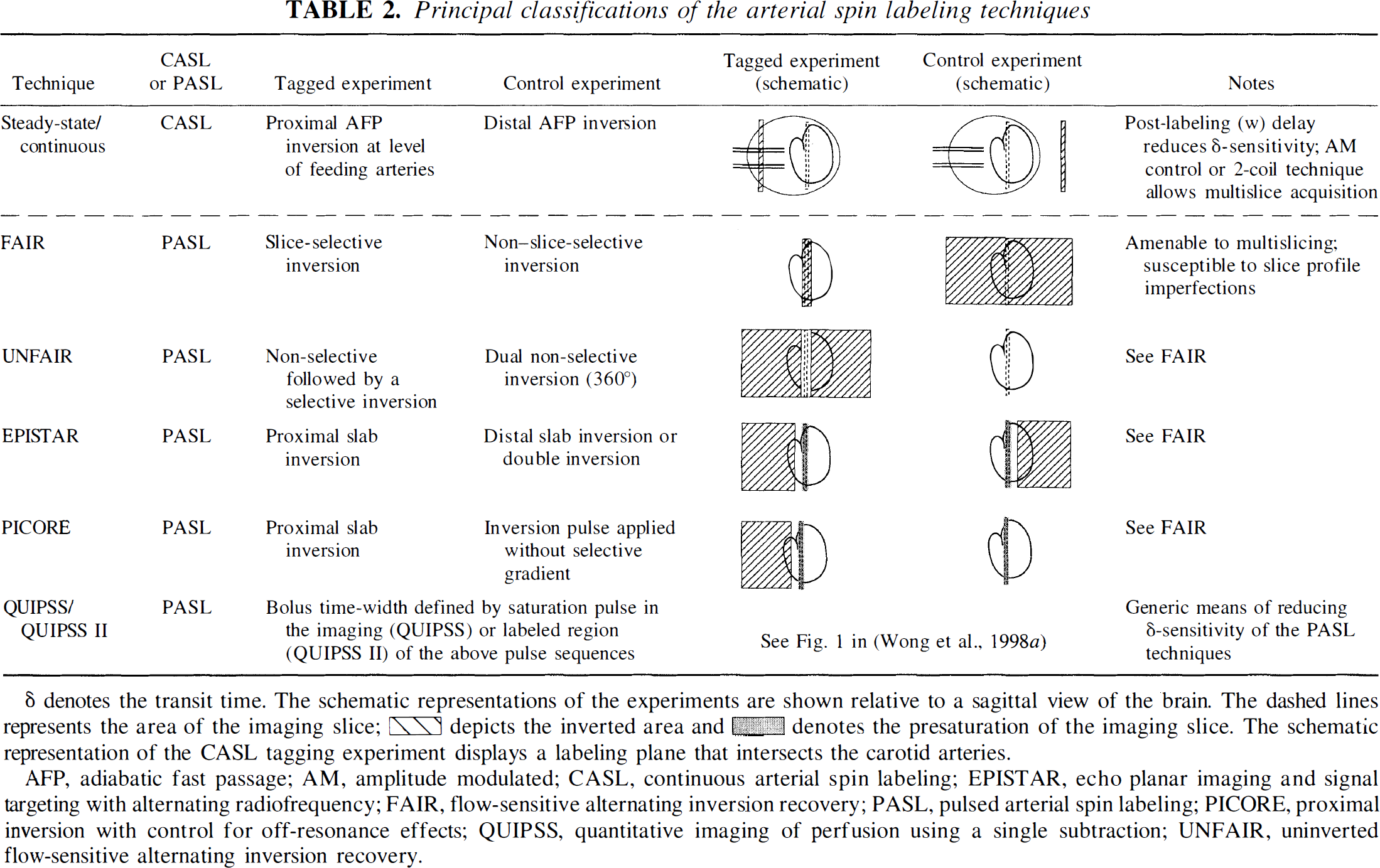
Transit time and magnetization transfer effects. Two main problems soon became apparent in the application of continuous spin labeling as a method to measure tissue perfusion accurately. First, the time taken for spins to travel between the labeling plane and the imaging slice (henceforth referred to as the transit time) is nonzero, and therefore T1 relaxation occurs during this period. Different regions of the brain have different transit times, depending on the distance from the labeling plane and the cerebrovascular anatomy. For accurate quantification, this effect must be taken into account. The transit time problem has been noted in experiments comparing CASL with the radioactive microsphere method of CBF quantification, where an underestimation of flow was observed with the spin labeling technique when the flow rates were low (Walsh et al., 1994). Second, the application of a long (i.e., several seconds) off-resonance RF pulse causes a decrease in the water signal resulting from magnetization transfer (MT) effects. Although no direct saturation of the observed water magnetization in the imaging slice occurs because of the narrow line width of the free water peak, saturation of macromolecular spins does occur, resulting in attenuation of the free water signal through magnetization transfer (Wolff and Balaban, 1989). This reduces the perfusion-dependent signal difference between the control and spin-labeled images. Zhang et al. (1992) made an initial attempt to account for these two effects by incorporating MT effects into the Bloch equation analysis and measuring the time lag between the initiation of spin labeling and the first observable decrease in tissue magnetization. They accounted for transit time effect by modifying the degree of inversion, α (equal to 0.5 for saturation, 1 for perfect inversion), by an amount related to T1 relaxation:
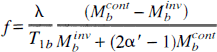
Magnetization transfer complicates the extension of the methods mentioned earlier to multislice acquisition, since the control image must experience exactly equivalent MT effects as the spin-labeled image. This means that the control “plane” must be symmetrically opposite the inversion plane with respect to the imaging slice, which can be true only for a single imaging slice, and limits the slice orientation to being perpendicular to the arteries in which spin labeling is performed. The control image is acquired by changing the sign of the frequency offset of the labeling pulse (assuming symmetrical MT effects) or by reversing the gradient polarity. It has been suggested (Pekar et al., 1996) that to properly account for MT effects (and possible eddy current effects caused by the labeling gradient) a four-step protocol for image acquisition should be used in which both frequency and gradient polarity are alternated, although this remains a point of debate (see Silva et al., 1997b). Alternatively, a two-coil setup can be used to avoid the saturation of macromolecular spins (Zhang et al., 1995). In this setup, a small surface coil is placed on the neck of the subject immediately adjacent to the artery supplying blood to the brain. The physical range of the B1 field produced by the surface coil is limited to a localized region. Arterial water spins are inverted using the surface coil, but no MT effects are observed in the brain, since the B1 field does not extend sufficiently far. A separate (actively decoupled) coil is used to apply the imaging pulses and receive signal. Extension of this approach to multislice perfusion imaging is straightforward, since the control image does not need to contain any MT information (Silva et al., 1995). However, specialized hardware is needed to implement this method, and flow quantification still is complicated by the need to account for a large range of arterial transit times. Recently, a more comprehensive analysis of the MT effects in single-coil CASL has been presented based on a four-compartment model of free and bound solvent and macromolecular protons (McLaughlin et al., 1997). Two alternative approaches for flow quantification were suggested, which differ in the way that the perfusion subtraction image is normalized and the manner in which T1 is measured. The presence of off-resonance radiation reduces the T1 of tissue caused by the MT effect, and the resulting relaxation time, T1sat, is an important parameter in this analysis. Complete saturation of the macromolecular magnetization is not a prerequisite of these approaches, making them directly relevant to the use of CASL in human studies, where RF power deposition is a restricting factor and macromolecular saturation cannot be guaranteed.
Intravascular signal. Another possible source of systematic error in CASL techniques is the presence of intravascular signal in the subtraction (control minus labeled) images. All of the theoretical models describing the relation between flow and signal difference (e.g., Eqs. 7 through 12) are based on the assumption that signal comes exclusively from tissue. If a significant amount of signal emanates from the vasculature, perfusion will be overestimated. Most spin labeling studies have been performed with flow-crushing gradients included in the imaging sequence, which are intended to completely eliminate signal from intravascular spins. Studies show that inclusion of a bipolar gradient pair with a “b” value (Le Bihan and Turner, 1992) of approximately 5 s/mm2 reduces the perfusion difference signal in human gray matter by almost 50% compared with the signal obtained with no crusher (Ye et al., 1997b). The extraction fraction, E, usually is assumed to be equal to unity (i.e., water is a freely diffusable tracer), and experiments by Silva et al. using CASL with and without macromolecular saturation (Silva et al., 1997a) and diffusion gradients (Silva et al., 1997b) demonstrate that this assumption is reasonable at normal flow rates in the rat brain. However, at higher flow levels, the extraction fraction was shown to be reduced (E ~ 0.6 when f = 400 mL 100 g−1 min−1). The transit time insensitive sequence proposed by Alsop and Detre (1996), mentioned previously, allows most of the labeled blood to either exchange with the tissue or “wash through” the vasculature during the postlabeling delay, and therefore suffers less from the associated errors of arterial signal contributions. Notice that since transit time effects cause an underestimation of CBF and intravascular signal causes an overestimation, the two effects can cancel out one another. However, this will be true only under specific circumstances, and both sources of systematic error need to be addressed. A combination of delayed acquisition and flow-crushing gradients seems to be sufficient to account for both effects (Ye et al., 1997a).
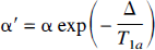
It has been suggested that the problems of intravascular signal contamination and extended transit times in regions of reduced perfusion can, paradoxically, be used to assist in the identification of these areas (Detre et al., 1998b). CASL approaches which include a postlabeling delay should achieve transit time insensitivity except in regions where the transit time is especially increased. These regions, which are likely to correspond to areas of extremely low perfusion, contain significant amounts of intravascular spin labeled water, and so in the ASL subtraction image appear as bright foci of signal (Fig. 9). Surrounding areas of moderately decreased CBF appear dark, reflecting the desired contrast for the perfusion image. Therefore, it is possible to identify the most severely compromised tissue based on the observation of unusually bright spots in the perfusion map. Quantitative interpretation of the signal is difficult, since knowledge of exact transit times is required, but qualitative evaluation of perfusion deficits should be possible, which may be adequate for clinical applications of the technique.
Intraluminal artifact in continuous arterial spin labeling (CASL) CBF subtraction images of stroke patients. Gray scale shows CBF ranging from 0 to 127 mL 100 g−1 min−1. 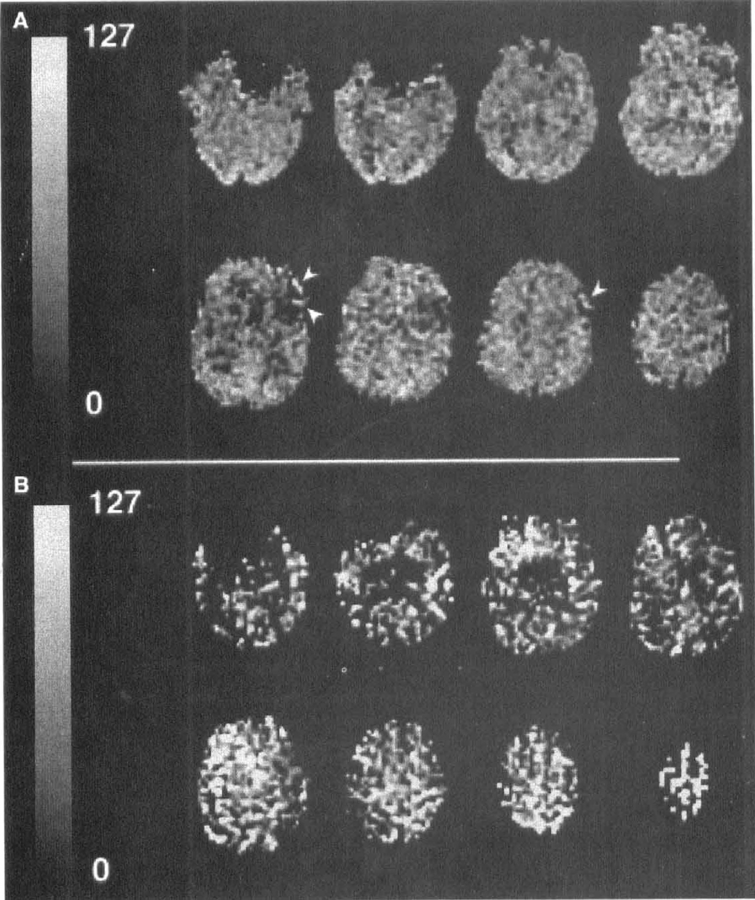
Multislice imaging. Finally, the extension of CASL techniques to multislice perfusion imaging with standard hardware has become possible with another method devised by Alsop and Detre (1998). Rather than acquiring the control image by changing the frequency or gradient polarity of the RF inversion pulse, the amplitude of the pulse is sinusoidally modulated at a certain frequency Φ. Fourier transformation of an RF waveform of base frequency Φ0 with sinusoidal amplitude modulation of frequency Φ results in a pair of inversion planes at frequencies Φ0 ± Φ. The result is that as spins flow through, they are inverted and then immediately “uninverted,” thereby losing their label. The MT effects of the sinusoidally modulated waveform have been shown to be equivalent to those of the standard labeling RF pulse (except close to plane of inversion), thus enabling multislice perfusion imaging with any image orientation. Some concerns remain regarding the efficacy of the double inversion pulse; however, it is likely that these problems will be overcome in the near future, making this technique extremely promising.
Pulsed arterial spin labeling techniques
Principal classifications of the arterial spin labeling techniques
ƍ denotes the transit time. The schematic representations of the experiments are shown relative to a sagittal view of the brain. The dashed lines represents the area of the imaging slice;  depicts the inverted area and
  denotes the presaturation of the imaging slice. The schematic representation of the CASL tagging experiment displays a labeling plane that intersects the carotid arteries.
AFP, adiabatic fast passage; AM, amplitude modulated; CASL, continuous arterial spin labeling; EPISTAR, echo planar imaging and signal targeting with alternating radiofrequency; FAIR, flow-sensitive alternating inversion recovery; PASL, pulsed arterial spin labeling; PICORE, proximal inversion with control for off-resonance effects; QUIPSS, quantitative imaging of perfusion using a single subtraction; UNFAIR, uninverted flow-sensitive alternating inversion recovery.
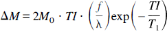
Echo planar imaging and signal targeting with alternating radiofrequency. The first of the PASL group of perfusion imaging approaches was proposed by Edelman et al. in 1994 and is known as echo planar imaging and signal targeting with alternating radiofrequency (EPISTAR) (Edelman et al., 1994). This technique is similar conceptually to CASL. After saturation of the imaging slice (see Transit Time Effects later), a slab proximal to the imaging slice is labeled using a single, short RF inversion pulse. The blood in this slab then is allowed to flow into the imaging slice, and an image is acquired after a time TI. A control image also is acquired for which the label is applied distal to the imaging slab (Edelman et al., 1994) or with no slab selective gradient (a variant known as PICORE [proximal inversion with control for off-resonance effects, Wong et al., 1997]). Recently, in an approach similar in concept to that of Alsop and Detre for CASL described in the previous section, the control image was acquired by applying a “double inversion” pulse pair (Edelman and Chen, 1998). The MT effect on the imaging slices is the same in the control and spin labeled images, and inflowing blood in the control image is fully relaxed, since it experiences an overall 0° nutation. Subtraction of the images results in a flow-dependent image with a signal intensity determined by (Kwong et al., 1995; Calamante et al., 1996):
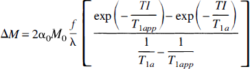
Flow-sensitive alternating inversion recovery. Measurements of changes in perfusion based on dynamic changes in tissue T1 were first performed by Kwong et al. (1992) (see Functional Brain Studies). However, measurements of resting values of perfusion were not possible using this method since the intrinsic tissue T1 was unknown. To identify the component of signal in the slice-selective inversion recovery image, which results purely from the inflow of blood spins during the inversion time, a second image is required, which has relaxed with intrinsic tissue T1. At approximately the same time, Kwong et al. (1995), Kim (1995), and Schwarzbauer et al. (1996) proposed the sequence that is commonly referred to as flow-sensitive alternating inversion recovery (FAIR). In this technique, two inversion recovery images are acquired. The first follows a slice-selective inversion and thus has a signal intensity determined by T1app (Eq. 9); the second follows a global inversion and so (assuming blood and tissue relax at the same rate) has no flow enhancement (i.e., the image signal intensity is determined by intrinsic tissue T1). Subtraction of the two images leaves a signal that is directly related to flow, and the relation is the same that as given earlier for EPISTAR (Eq. 13). In the general case when T1app ≠ T1a, the biexponential expression of Eq. 14 applies. This is true because EPISTAR and FAIR are equivalent insofar as they involve the acquisition of a pair of images, one of which has inverted blood water flowing into the imaging slice and the other of which has fully relaxed blood water flowing in. In the two techniques, the state of the static tissue magnetization is different at the time of image acquisition (FAIR images derive from an inversion recovery, whereas in EPISTAR the tissue is saturated before the application of the inversion tag). However, since the static component of the signal is removed by subtraction of the spin-labeled image from the control image, the behavior of the difference signal with inversion time is the same in both techniques (Fig. 10).
Raw spin-labeled images and difference images (control-labeled) of the human brain for EPI and signal targeting with alternating radiofrequency (EPISTAR) and FAIR as a function of inversion time (TI). From top to bottom: EPISTAR raw images; FAIR raw images; EPISTAR difference images; FAIR difference images. The TI values from left to right are as follows: 200, 400, 600, 800, 1000, and 1200 milliseconds. Whereas the static tissue contrast is different for the two techniques, the difference images are dependent only on the inflow of labeled blood. (Reprinted from Wong et al.[1997] Implementation of quantitative perfusion imaging techniques for functional brain mapping using pulsed arterial spin labeling. NMR Biomed 10:237–249. Copyright John Wiley & Sons Limited. Reproduced with permission.)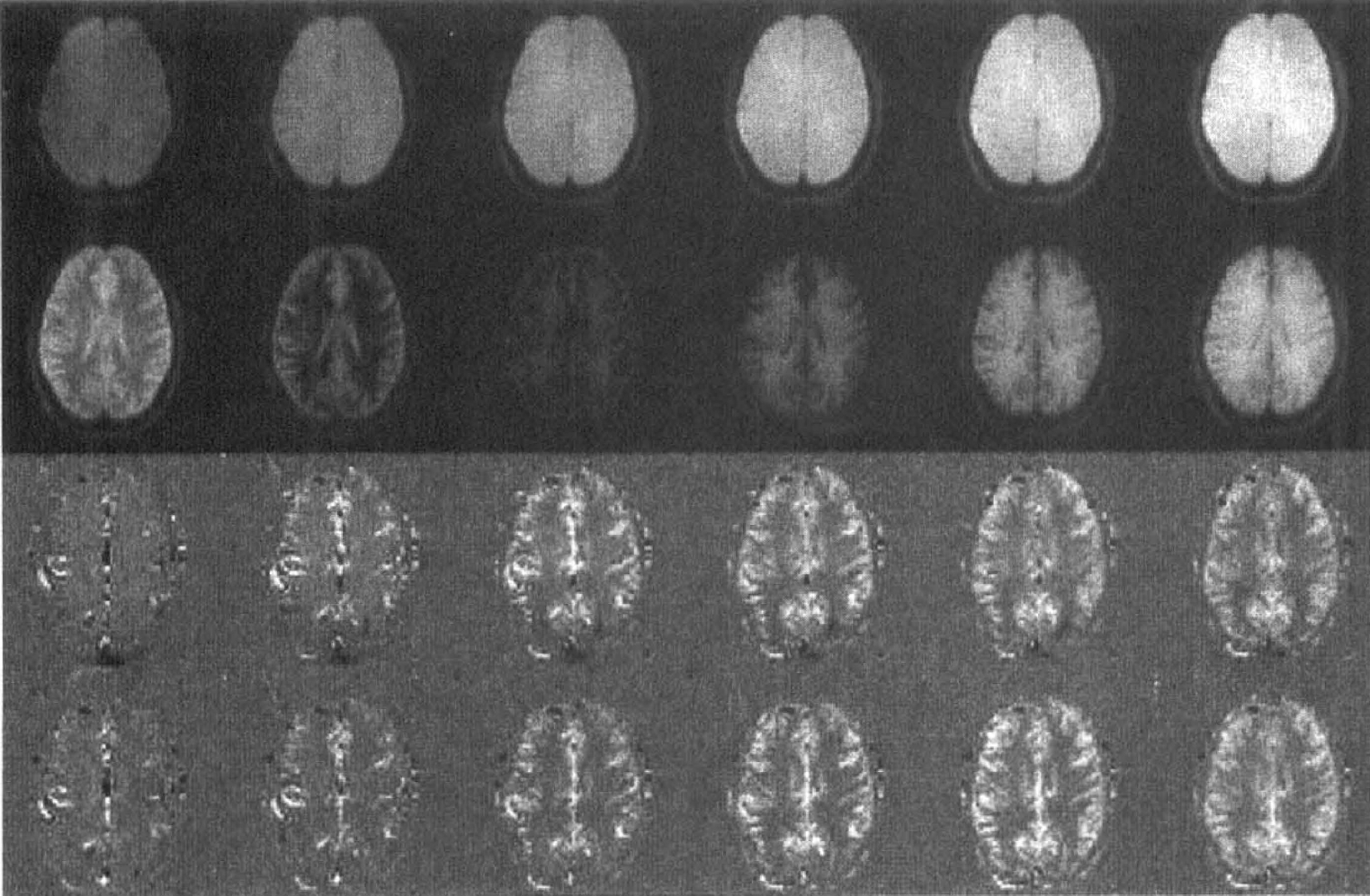
Transit time effects. A practical consideration for both EPISTAR and FAIR is the interaction of the edges of the inversion slice with the imaging slice. Ideally, the slice profiles of both the imaging and inversion pulses would be sharp “top-hat” functions, and the inversion slice would be placed immediately adjacent to (for EPISTAR) or superimposed over (for FAIR) the imaging slice. However, the actual inversion profiles generated by hyperbolic secant (sech) adiabatic RF pulses are not perfectly rectangular. The edges of the inversion slice have a certain degree of slope caused by the transition between spins meeting and not meeting the adiabatic condition. Spin relaxation during the play out of the pulse also can degrade the shape of the pulse profile (Frank et al., 1997). To minimize the interaction between the inversion and imaging slice profiles, EPISTAR usually is implemented with an in-plane RF presaturation pulse of thickness slightly greater than the imaging slice, applied immediately before spin labeling (Table 2). Also, it is necessary to move the edges of the inversion slice away from the imaging slice, which means that the inversion slice is shifted away from the imaging slice for EPISTAR and widened for FAIR. A typical inversion–imaging slice thickness ration that has been used in FAIR is 3:1 (Kim, 1995), which was found to be the minimum necessary to avoid subtraction artefacts from static tissue signal. As a result of this, a transit time is introduced during which the inflowing blood is not in the state assumed by the standard model (fully relaxed for FAIR, fully inverted for EPISTAR). Attempts have been made to minimize the inversion–imaging slice thickness ratio by using frequency offset corrected inversion (FOCI) adiabatic pulses (Ordidge et al., 1996) for improved slice definition in FAIR (Pell et al., 1998; Yongbi et al., 1998). A second practical point to consider is the width of the inverted slab of spins. If the bolus width is insufficiently wide, fresh spins that have not been inverted will flow into the imaging slice during the inversion time. In EPISTAR, this width is defined in the pulse sequence by the band width of the inversion pulse and the slice-select gradient; in FAIR, the range of spins affected by the nonselective inversion pulse is defined by the physical extent of the RF coil. If inflow of fresh spins occurs, the perfusion signal will be less than predicted by the standard ASL model. Therefore, the presence of either a transit time or inflow affects the accuracy of perfusion quantification (Kim et al., 1997b; Pell et al., 1999a).
An alternative kinetic model has been put forward by Buxton et al. (1998) to describe the behavior of the signal difference in pulsed and continuous ASL experiments, which takes into account a finite transit time and limited bolus width. These factors can be incorporated into the standard T1 model described earlier (Kim et al., 1997b; Pell et al., 1999a), leading to similar predictions for the behavior of ΔM as a function of inversion time for the two models. Although generally less than in continuous ASL, the transit time in pulsed ASL can be large, particularly in multislice acquisitions. Using standard PASL techniques, it is necessary to acquire image pairs at a range of inversion times to estimate the transit time and account for its effect on perfusion quantification. Alternatively, PASL pulse sequences can be modified to reduce their sensitivity to transit time effects and allow the acquisition of a purely perfusion-dependent subtraction image. The most promising of these modifications have been proposed by Wong et al. under the acronyms QUIPSS (Quantitative Imaging of Perfusion using a Single Subtraction) and QUIPSS II (Wong et al., 1998a). In QUIPSS, a saturation pulse is applied to the imaging slice at a time TI1 after application of the labeling or control RF pulse, and the image is acquired at a later time TI2. By doing this, any signal difference that evolves during TI1 is destroyed, and only spins that enter during the subsequent period ΔTI (= TI2 – TI1) before image acquisition contribute to the perfusion difference signal. Under these circumstances, perfusion quantification is transit time independent as long as TI1 is longer than the longest transit time of the system, and ΔTI is less than the temporal width of the remaining spin-labeled bolus. In QUIPSS II, a saturation pulse is applied to the labeled region at time TI1, effectively “clipping” the trailing edge of the bolus and thus giving it a well-defined temporal width, and the image is again acquired at TI2. For this sequence, the conditions for transit time insensitivity are as follows: (1) TI1 must be less than the natural width of the labeled bolus, and (2) ΔTI must be greater than the longest transit time of the system so that the entire bolus enters the imaging slice before the image acquisition. The conditions for QUIPSS II are more easily met than for QUIPSS, and QUIPSS II also has the advantage of allowing some washout of labeled intravascular signal during the ΔTI period. Contamination of the perfusion signal by the signal from labeled blood in large vessels is minimized, resulting in a more accurate measurement of tissue perfusion. The drawback of the technique is a reduction of the perfusion signal difference compared with standard PASL techniques because of T1 decay during ΔTI.
The introduction of a transit time-insensitive PASL sequence has allowed the extension of the technique to multislice acquisitions. Initially, FAIR was implemented in a multislice mode merely by increasing the width of the slice-selective inversion so that several slices were contained within the inversion slab (Kim and Tsekos, 1997a). Also, EPISTAR has been used to obtain multislice perfusion data by acquiring several image slices adjacent to the inversion slab (Edelman and Chen, 1998). However, in these approaches, a range of transit times is automatically introduced by the different physical distances between each imaging slice and the closest edge of the inversion slice, thus making accurate quantification difficult. For multi slice PASL, QUIPSS II is a natural choice because of its inherent transit time insensitivity. The main problem for QUIPSS II is the need to limit the second inflow time ΔTI to a length that is not much longer than tissue T1 to prevent the decay of a significant proportion of the perfusion label. Since the condition for transit time insensitivity is that ΔTI is longer than the longest transit time present, a limitation on the length of ΔTI limits the robustness of the sequence and, therefore, limits the number of slices that can obtained in a single acquisition.
Intravascular signal. As with CASL, the contribution of blood water signal needs to be considered in the quantification of the PASL difference signal. The inclusion of a bipolar gradient in the imaging sequence has been shown to reduce the perfusion signal and cause a lengthening of the measured transit time (Wong et al., 1998b). This is interpreted as a reduction in the amount of spin-labeled blood water signal present in the subtraction images, since the rapid motion of the intravascular water should cause its signal to decay rapidly in the presence of a field gradient. However, choice of the magnitude of the gradient strength (or “b” value) is arbitrary and generally is empirically determined as the point at which a further increase in b value does not alter the calculated perfusion value. There remains some debate in the literature as to whether blood signal should contribute in any way to the perfusion signal. In the original T1 model for ASL, it is assumed that all signal originates from tissue water, since CBV is relatively small and crusher gradients are used. However, it has been suggested (Buxton et al., 1998) that blood water, which is contained within a voxel in the imaging slice and ultimately is destined to perfuse that voxel but which at the time of image acquisition still is in the intravascular space, should be contribute to the PASL signal. This is distinct from blood that is merely passing through a voxel in an artery or arteriole and is traveling to a capillary bed outside of that voxel; this blood should not be included in the perfusion signal. If the signal from intravascular, perfusing blood is not acquired, a quantity slightly different to absolute perfusion is measured. The measurement represents the water extraction fraction–flow product E(f) · f (Zaharchuk et al., 1998). In the situation where the extraction fraction is approximately equal to unity, which is true under normal circumstances, this product is equivalent to CBF. However, at higher flow rates where the extraction fraction is known to deviate substantially from unity, a misleading result will be obtained if exclusively tissue water signal is acquired.
In practice, the relative contribution of tissue and blood signal is difficult to assess, since the source of signal is not easily identified. If a bipolar crusher gradient is applied, calculations may be performed to estimate the attenuation of randomly diffusing water signal, although how directly this relates to blood traveling through the arteriole–capillary–venule system is unclear. Complete elimination of signal from blood traveling through a voxel, while simultaneously leaving perfusing intravascular water signal unaffected, is not possible with the use of bipolar gradients (Henkelman, 1994). The extent to which slowly flowing capillary water is attenuated depends on factors such as the exact flow rate and vessel geometry. If blood water signal does contribute to the PASL perfusion signal, a secondary complicating effect is introduced by the different T2 (or T2*) values for blood water spins and tissue water spins. In the human brain, T2 of intravascular water has been estimated to be a factor of approximately 3 greater than that of tissue water (240 versus 80 milliseconds at 1.5 T in Buxton et al., 1998). This could pose a problem for methods that use EPI for image acquisition, since at any given echo time the signal will be weighted toward the intravascular compartment. For a multi-TI experiment, where spin-labeled water progressively shifts from the intravascular to tissue compartments as the inversion time increases, this introduces a systematic bias to the data. This problem has not been addressed in the literature but could potentially affect the values of perfusion obtained using ASL substantially, depending on the intravascular lifetime of spin-labeled water in voxels in the imaging slice. If TurboFLASH (Haase, 1990) image acquisition is used, the problem is minimized because of the extremely short echo times used; however, T1 relaxation during the imaging period and the saturation effects of repeated RF excitation pulses make the quantification of TurboFLASH ASL images subject to the validity of certain assumptions (e.g., that the image contrast is dominated by the central lines of k-space). Also, TurboFLASH is not amenable to rapid multislice imaging.
Alternative pulsed arterial spin labeling methods. Since the introduction of EPISTAR and FAIR several years ago, a range of methods has been proposed based on the concept of PASL. For example, Un-inverted flow-sensitive alternating inversion recovery (UNFAIR) (Helpern et al., 1997b) is an approach similar to FAIR but modified so that the static tissue component of the signal remains at equilibrium rather than being inverted in both the spin-labeled and control images (Table 2). Other suggested approaches include STAR-HASTE (Chen et al., 1997), PARIS (Helpern et al., 1997a), TILT (Golay et al., 1998), BASE (Schwarzbauer and Heinke, 1998), SMART (Kao et al., 1998), and FAIRER (Zhou et al., 1998). The relative benefits and drawbacks of each of these methods have yet to be fully established, and the reader is referred to the relevant references for details of each of the sequences.
Other arterial spin labeling quantification issues
Accurate quantification of perfusion with the ASL techniques in animals and humans requires consideration of several additional factors. These factors are summarized here:
Implementation of the CASL method on clinical scanners: Initial studies using CASL were performed on small animals, where the problems associated with transit times and MT effects are minimal. The clinical implementation is hampered by the increased magnitude of the transit times in humans. Loss of the label also is intensified by the shorter longitudinal relaxation times at the typically lower field strengths. A further issue is related to RF power deposition. The limits on the duty cycle of RF amplifiers and the specific absorption rate of the sequence often restrict the application of a continuous pulse over the required duration (several seconds). Instead, a pulse train is applied consisting of repeated rectangular pulses with a duty cycle of approximately 75% to 90% (Roberts et al., 1994; Ye et al., 1997). Degree of inversion, α: An accurate measurement of α is necessary for both continuous and pulsed ASL. The method of α determination described by Zhang et al (1993) has been criticized over the measurement location and the bias toward the lower range of laminar flow velocities present in the carotid artery (Maccotta et al., 1997). The degree of inversion is considerably more velocity-dependent for the CASL technique than for the pulsed techniques (Wong et al., 1998b), since the fulfillment of the adiabatic condition in the case of the continuous adiabatic fast passage pulse is intrinsically related to the velocity of spin passage through the labeling gradient (Dixon et al., 1986). Individual calibration of the value of may, therefore, be necessary for the CASL technique. Blood–brain partition coefficient, λ: A uniform value of λ often is assumed in previous studies of CBF quantification, but this may be an unrealistic assumption. Different values of the partition coefficient have been reported for gray and white matter and for varying hematocrit levels (Herscovitch et al., 1985). It is also possible that the regional values of λ will vary as a consequence of evolving pathophysiologic mechanisms. An imaging method for λ determination on a pixel-by-pixel basis has been described (Roberts et al., 1996). BOLD contrast: Simultaneous flow and T2*-contrast information can be extracted from a GE-based ASL experiment. Several groups have used FAIR (Kim et al., 1997b, c; Zhu et al., 1998) and QUIPSS (Wong et al., 1997) to study the combined flow and BOLD responses to functional activation paradigms. For flow quantification studies using GE or SE image acquisition, the respective T2*- or T2-weighting of the signal must be extracted (see Intravascular Signal), and this procedure usually is based on baseline measurements (Kim, 1995). CSP contamination: The partial volume effect of CSF, which is exacerbated with the larger voxel sizes used in clinical imaging, can result in significant underestimation of flow. Kwong et al. (1995) predicted an underestimation of approximately 30% for a gray matter–CSF volume fraction of 50%:50%. T1 of blood, T1a: The measurement of flow with ASL requires a determination of T1a. Previous studies report a value of this parameter by extrapolation from published in vitro data. The dependence of T1a on factors such as oxygenation, hematocrit, vessel size, and environment may be significant and requires further study. Venous contamination: The blood in the venous circulation during the experiment may have been labeled by the control or labeling experiments and thereby provide an unwanted contribution to the subtraction signal. This depends on the chosen labeling scheme. Geometrical layout of the tagged vasculature: Early implementations of the CASL technique used a labeling plane in the neck that is perpendicular to the direction of the feeding artery. To reduce the transit time, the labeling plane can be displaced to the level of the blood vessels that lie at the base of the brain (Alsop et al., 1996; Ye et al., 1997b), but the component of the blood velocity along the direction of the labeling gradient must be sufficient to fulfill the adiabatic condition. For both pulsed and continuous techniques, an indirect path of the blood to the imaging slice is reflected as a longer transit time. The techniques are not sensitized to blood that remains in vessels running parallel to and within the imaging slice during the course of the experiment.
ARTERIAL SPIN LABELING APPLICATIONS
Cerebrovascular disease
Since the establishment of the ability of the techniques to reflect tissue perfusion status, ASL has been used increasingly as an experimental tool in several areas of investigation. The quantitative accuracy of the flow measurements of pulsed and continuous techniques has been investigated using animal and human studies (Table 1). Although pulsed ASL has almost exclusively been used in the field of functional magnetic resonance imaging (fMRI) (see Functional Brain Mapping), continuous ASL also has been successively applied to studies of cerebrovascular disease, both in experimental and clinical settings. This section briefly summarizes the main applications of ASL.
Soon after the technique was proposed, CASL was used by Jiang et al. (1993) in a rat model of transient MCAO and by Detre et al (1993) to demonstrate the redistribution of blood flow through anastomoses after unilateral occlusion of the common carotid artery in the rat. By labeling blood flowing through the unoccluded artery only, the effective territory of that artery and how the territory changed after occlusion of the other artery was shown. In the following year, Jiang et al. (1994) performed a study in which they monitored the effect of whole-body hypothermia on the recovery of perfusion after transient MCAO. Cerebral blood flow was measured quantitatively by CASL with a time resolution of 8.5 minutes using a standard spin echo imaging approach, and it was shown that the degree of postischemic hypoperfusion is reduced if hypothermic conditioning is applied. The same group recently used CASL to study reperfusion levels after anti-intercellular adhesion molecule 1 antibody treatment of MCAO in the rat (Jiang et al., 1998b) and to investigate the thrombolysis of embolic stroke after administration of rt-PA (Jiang et al., 1998a), again in the rat brain. Busch et al. also studied the effect of rt-PA on an embolic stroke insult (Busch et al., 1998), comparing the results from ASL perfusion with ADC measurements. Their results show that an improvement in blood flow as shown by the ASL perfusion maps led to a slowly progressing reversal of ADC changes in the periphery of the ischemic territory, indicative of tissue recovery. In an experiment looking at the acute changes of tissue relaxation parameters after MCAO, Calamante et al. (1999) used CASL perfusion mapping to identify the extent and the severity of ischemia in the affected MCA territory. In a similar study, CASL was used to characterize the changes observed in a model of partial MCAO (Fig. 11). Our group also has been using FAIR perfusion imaging in the study of global ischemia–reperfusion time courses (Pell et al., 1999a). In these experiments, perfusion was measured with a time resolution of 4 minutes, allowing a period of acute postischemic recovery of flow to be defined, followed by a prolonged period of hypoperfusion (Fig. 12). The combination of CBV and CBF measurements with the techniques of contrast agent MRI and CASL, respectively, has been made possible by the development of a contrast agent with modified susceptibility characteristics (Zaharchuk et al., 1998). A study of the flow and volume response to MCAO in the rat was thereby undertaken. Forbes et al. (1997) used ASL to measure CBF and CO2 reactivity after traumatic brain injury caused by controlled cortical impact. All of these studies demonstrate the ability of ASL methods to provide time courses of perfusion measurements with good temporal resolution in a series of individual subjects.
An example of the ability of CASL to differentiate between different levels of CBF. The top row shows blood flow in an coronal slice of a rat brain before Reperfusion time courses in a gerbil model of transient forebrain ischemia (n = 8). Measurements were performed using a modified version of FAIR with improved time efficiency (Pell 1999a). The control blood flow measurements were 158 ± 24 mL 100 g−1 min−1 in the cortex and 130 ±17 mL 100 g−1 min−1 in the striatum. On initiation of recirculation, the blood flow recovered and, at approximately 5 minutes of reflow, reached a maximal level; a period of hypoperfusion followed. An expotentially damped polynomial model was fitted to the first 60 minutes of postocclusion data (dark line) to characterize features of the flow response during the acute stage of the reperfusion (Pell et al. 1999b).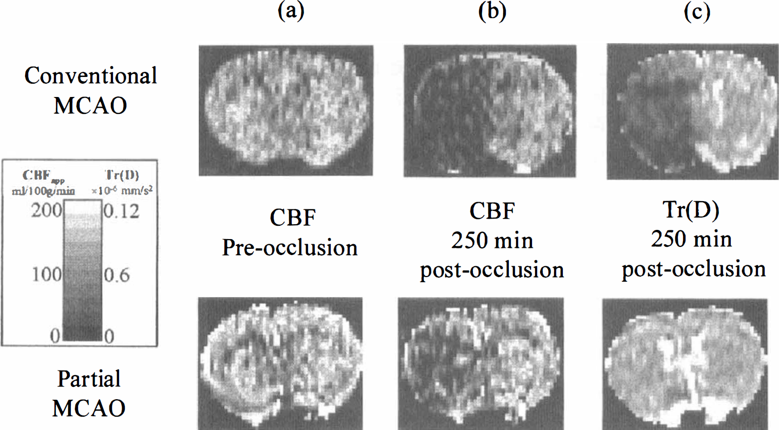
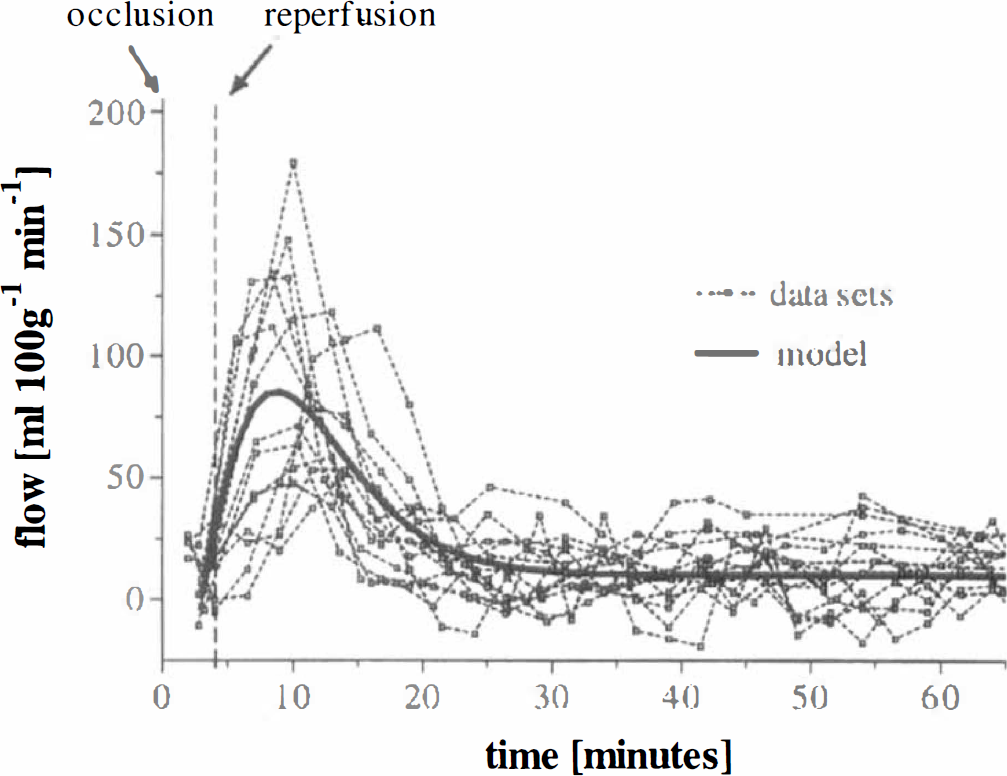
In the clinical environment, initial efforts have been made by Detre et al. (1998a) to determine cerebrovascular reserve by assessing the response of the CASL flow measurement to ACZ. The group also has used the technique to evaluate CBF deficits in patients who presented with stenoses and cerebrovascular accidents (Detre et al., 1998b). Evidence of watershed hypoperfusion was found. Similar attempts have been made for EPISTAR (Siewert et al., 1997). However, both techniques have the inherent problems associated with long arterial transit times, and quantitative blood flow measurements have not been reported. Table 1 summarizes the flow values obtained by quantification studies using the ASL techniques.
Functional brain mapping
Initial studies. Since the pioneering work of Roy and Sherrington (1890), it has been known that there is a close spatial and temporal correspondence between local changes in brain neuronal activity and changes in regional cerebral blood flow (rCBF). Whereas the mechanisms of this flow regulation still are poorly understood in detail (Villringer and Dirnagl, 1995), it is well established that blood flow typically changes by 50% or more in gray matter within an area close to that of increased electrical activity (Puce, 1995) and within a few seconds of the onset of increased activity. The well-established technique of PET (Frackowiak et al., 1997) has been used since the early 1980s to monitor rCBF during functional brain activation and is regarded by some as a gold standard for such measurements. The new MRI techniques discussed in this review, measuring ostensibly the same parameter, can be regarded as directly comparable with PET. This is not the case with the more popular fMRI technique of BOLD contrast, which uses the paramagnetic properties of deoxyhemoglobin. Here, the functionally induced image intensity may depend on several parameters, including blood flow, oxygen extraction, hematocrit, local vascular geometry, and baseline blood oxygen saturation. In the special case of SE BOLD contrast (van Zijl et al., 1998), quantification appears to be possible, but this technique has low sensitivity except at high magnetic fields.
The first study using MRI perfusion techniques to observe functional activity in human brain was made by Belliveau et al. (1991). The contrast agent bolus passage method was used, with two venous injections of gadolinium spaced 20 minutes apart. Echo planar imaging was used to monitor the passage of the agent, with a repeat time of 1 second. During the first injection, the subject lay in darkness, whereas during the second he was given visual stimulation with flashing light–emitting diodes. The images from each injection were transformed into relative blood volume maps, and the map made when the subject was in darkness was subtracted from that made during visual stimulation. A significant increase of blood volume in occipital cortex was observed, consistent with PET and other studies of human cerebral visual areas. No attempt was made to quantify perfusion changes in this study. Because of the potential toxicity of gadolinium in repeated doses large enough to give adequate signal changes—only two scans per day can be performed—this technique has not found popularity in functional brain mapping studies.
However, this first publication aroused enormous international interest in MRI as a means of exploring human brain function, and it was not long before the technique of BOLD imaging, using the inherent magnetic properties of deoxyhemoglobin, nature's own contrast agent, was invented by Ogawa (1990) and Turner (1991), working with animal models. Kwong (1992) and Ogawa (1992) soon demonstrated the extreme power of this method in mapping human brain activity, again using visual stimulation. However, in addition to the use of BOLD, Kwong et al. (1992), using an early version of ASL, also obtained results that were entirely consistent with their BOLD data (Fig. 13). The method used RF pulses to invert the spins within the slice to be imaged, and an inversion time of 1100 milliseconds was used to allow noninverted perfusing spins time to move into the imaging slice. This technique is not capable of giving an absolute measure of blood flow, but using Detre's (1992) formalism, Kwong et al. were able to estimate the change of blood flow in occipital cortex produced by visual stimulation. This gave a result (ΔCBF = 55 mL 100 g−1 min−1), which is consistent with earlier PET studies. Characteristically, however, the sensitivity of this technique was lower than with BOLD contrast. The next development was made by Edelman et al. (1994), who introduced and applied EPISTAR (see Pulsed Arterial Spin Labeling Techniques) to study local brain activity produced by finger tapping.
Noninvasive, real-time mapping of V1 activation during visual stimulation. Images are obliquely aligned along the calcarine fissure with the occipital pole at the bottom. Images were acquired at 3.5-second intervals using a slice-selective inversion-recovery sequence. A baseline image acquired during darkness (upper left) was subtracted from subsequent images. Eight of these subtraction images are displayed and were chosen when the image intensities reached a steady-state level, during darkness (OFF), and during 8-Hz photic stimulation (ON). During stimulation, local increases in signal intensity are detected in the medial–posterior regions of the occipital lobes along the calcarine fissure. (Reprinted from Kwong et al. [1992] Dynamic magnetic resonance imaging of human brain activity during primary sensory stimulation. Proc Natl Acad Sci USA 89:5675–5679 with permission.)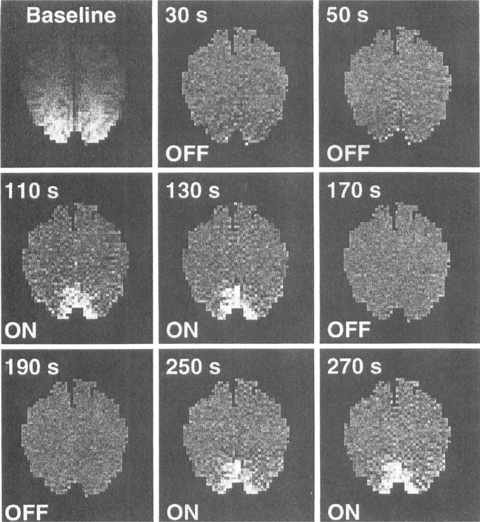
Imaging neuroscience studies in humans with arterial spin labeling. A further conspicuous advantage of EPISTAR and other ASL techniques over BOLD and bolus passage contrast agent methods is that the label produced by RF inversion of arterial spins is short lived, lasting only long enough to be observed in capillaries in the imaging slice of interest. Thus, minimal label passes downstream into veins, in contrast with the other methods, and hence ASL techniques have been claimed to provide better spatial specificity for cortical activations. This inspired a more advanced series of experiments on human hand movement using the EPISTAR method (Sanes et al., 1995), which considered the question of somatotopy in M1. Conventional wisdom, dating from Penfield and Boldrey's (1937) work, suggests that motor representations of the digits lay in an orderly sequence along the anterior wall of the central sulcus and the adjacent precentral gyrus. Sanes et al. (1995) were able to show that movements of individual digits each activated overlapping mosaics of areas scattered through the overall hand representation with little or no signs of a spatial sequence, a result consistent with single electrode studies on monkeys by Merzenich and his group (Nudo et al., 1992). In addition, EPISTAR was used to identify the frontal eye fields in a visual saccade task (Darby et al., 1996).
These successes triggered increased efforts to make ASL more quantitative, and thus a more complete alternative to PET. A variety of techniques involving different patterns of RF pulses have been developed. Several of the studies involving specific brain tasks have been undertaken by the group of McLaughlin at the National Institutes of Health using the CASL technique. Whether the local changes in CBF seen using the relatively high spatial resolution of MRI methods is comparable with that obtained using PET is of interest. The first of these studies (Ye et al., 1997c) measured rCBF changes in motor cortex with a finger-tapping paradigm. Without spatial smoothing, the spatial resolution of the functional images was about 4 mm, and the mean change in CBF over five subjects was 91%, considerably larger than that noted using PET (Fig. 14). This value was confirmed in a similar study by Kim et al. (1997a) using the FAIR technique. However, when images were smoothed to a full width at half maximum of 15 mm, more typical of multisubject PET studies, the mean ΔCBF fell to 42%, now in agreement with previously reported 133Xe and PET studies. This strongly suggests that earlier non-MRI studies have been prone to underestimate ΔCBF because of uncorrected partial volume effects. A further study by this group (Ye et al., 1998) investigated a more cognitive, working memory task, involving button press responses to numbers presented on a screen two steps previously—the “two-back” task. This ASL study reproduced results using BOLD well but also provided a significant confirmation of the PET finding that ΔCBF (23% averaged over six subjects in this study) is considerably lower in activated prefrontal cortical areas known to support working memory than blood flow changes in more primary cortex.
Cerebral blood flow activation images for seven control subjects using the CASL technique. The CBF measurements were convolved with a Gaussian kernel having a full width half maximum of 5.6 mm. Regions marked in black overlay had statistically significant differences in CBF during finger tapping. (Reprinted from Ye et al. [1997] Quantification of regional cerebral blood flow increases during motor activation: a steady-state arterial spin-tagging study. Neuroimage 6:104–112 with permission.)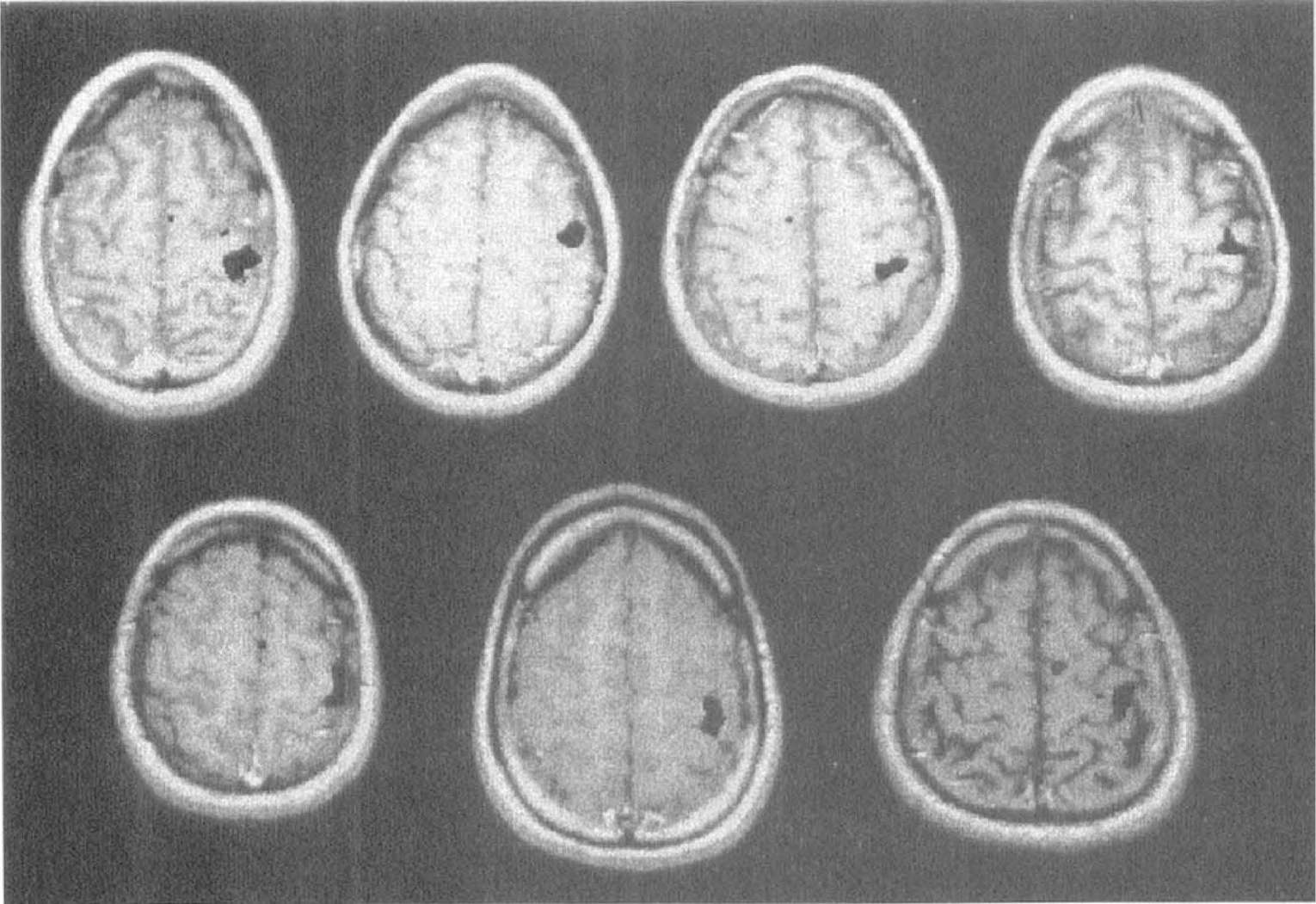
For functional studies, imaging more than a single slice of the brain in each experimental run clearly is of value (Kim et al., 1997b, Wong et al., 1997). This is discussed more fully elsewhere in this review, but the careful study extending coverage to 10 slices using FAIR with spiral EPI (Yang et al., 1998) is worthy of note. In this study, the areas of increased CBF for a finger movement task were shown to be similar to those found with BOLD contrast, confirming earlier work (Siewert et al, 1996).
Functional arterial spin labeling studies in animals. Meanwhile, functional studies using laboratory animals were being conducted in several laboratories. These investigations have increased understanding of the neurophysiologic basis of BOLD contrast. Kerskens et al. (1996) adapted a rat model showing increases in blood flow using CASL in somatosensory cortex during forepaw stimulation. The CBF effects of various types of anesthesia also were studied. They found that a-chloralose anesthesia best ensures persistence of CBF autoregulation to observe effects of hypercapnia on local blood flow changes (Bock et al., 1998). Surprisingly, they found that although the local blood flow increase induced by forepaw stimulation increased by 40% under hypercapnic conditions, there was no significant change in the BOLD contrast signal associated with the stimulation. This is consistent with the hypothesis that when blood flow is globally increased by hypercapnia, during activation local perfusion and oxygen extraction also increase in parallel. These results disagree with those obtained using PET in human brain with a visual stimulus (Ramsay et al., 1993), which showed no variation of local blood flow increase with hypercapnically induced changes in global blood flow. The sources of the discrepancy may be species differences in vascular density and regulation mechanisms.
Another important study (Schmitz et al., 1998) deals with the recovery of rat cerebral vascular autoregulation after cardiac arrest. One hour after successful resuscitation after 10 minutes of cardiac arrest, the ADC did not differ from control, but functional activation associated again with forepaw stimulation was completely suppressed. After 3 hours of reperfusion, functional activity began to reappear, but the recovery of the BOLD signal progressed faster than that of the CASL perfusion-weighted signal. On previous rat studies using electrophysiologic methods and laser Doppler flowmetry, this group found that cortical electrical activity also was slow to recover after cardiac arrest and was mirrored precisely by the recovery in rCBF.
Silva et al. (1995) were the first to perform pharmacologic fMRI using perfusion techniques in a rat model. They examined the CBF response to amphetamine using the two-coil CASL method and found that amphetamine causes significant and spatially specific increases in perfusion in many areas of the brain, including the cortex, cingulate, and caudate putamen (Fig. 15), in agreement with previous results using deoxyglucose uptake to monitor brain activation. This pioneering study indicates the power of perfusion methods to indicate in a simple way the localization of the effect of psychopharmaceutical agents in the brain, although care must be taken to control for any global effects on blood flow caused by the crude vasoactive properties of such drugs. Later work from the same laboratory (Forman et al., 1998) used picrotoxinin (a gamma-aminobutyric acid antagonist) to stimulate rat brain, whereas perfusion was measured by CASL, and brain glutamate was independently assayed using microdialysis. After 30 minutes of picrotoxinin-induced stimulation, glutamate levels decreased but CBF was found to remain elevated, suggesting that additional factors modulate the relation between neuronal neurotransmitters and hemodynamics at these later stages.
Five-slice perfusion images (two-coil CASL technique) of a rat brain before and after the intraperitoneal administration of 20 mg/kg of D-amphetamine in saline: 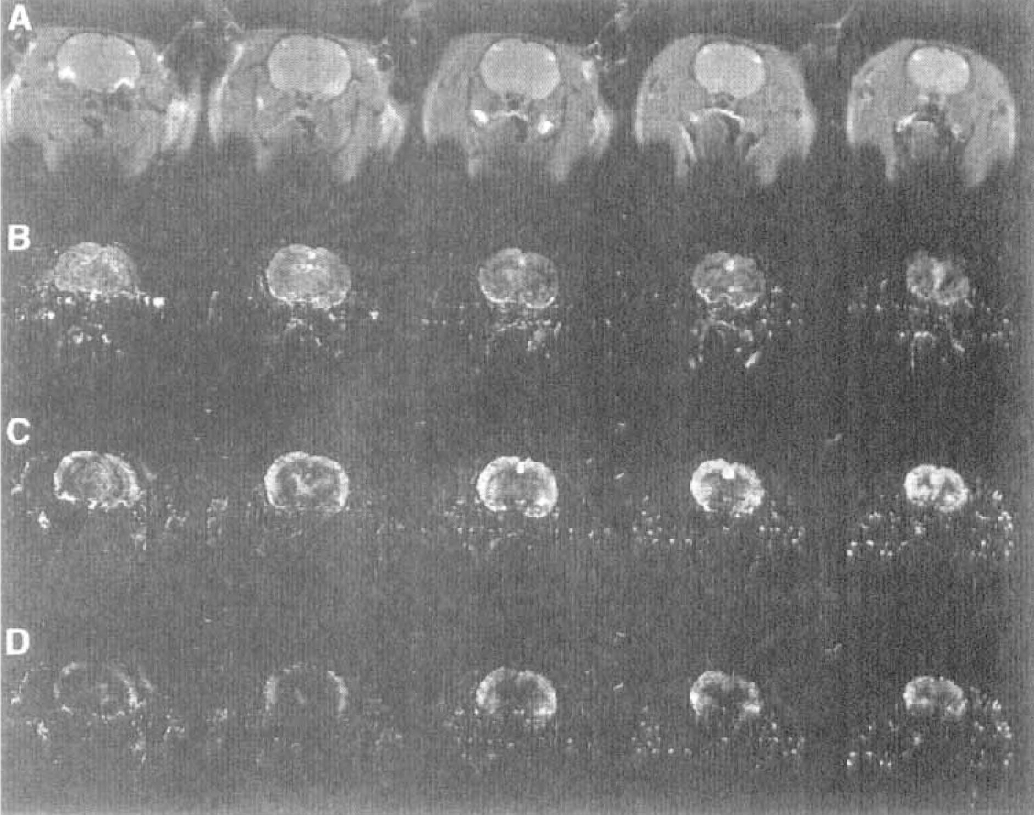
Although such studies clearly have great potential for understanding regional effects of drugs affecting neurotransmission, major gaps exist in our understanding of the normal energy-providing mechanisms for brain functional activity. Coupled with BOLD contrast, ASL seems likely to shed considerable light on the question of coupling of changes in neuronal activity, CBF, and oxygen extraction. Kim and Ugurbil (1997c) were the first to make quantitative studies of the differences in amplitude between BOLD and FAIR perfusion measures of activation. They report that BOLD signal change is not linearly correlated with the relative CBF increase across the subjects they studied and is negatively correlated with the oxygen consumption change they estimated using the Ogawa (Ogawa et al., 1993) model of the BOLD effect.
Later work by Davis et al. (1998) used the effects of hypercapnia, which is not thought to increase cortical oxygen consumption, on ASL and BOLD measurements to calibrate these measures for subsequent functional activation studies (Fig. 16). This calibration procedure provided a regional measurement of the expected sensitivity of the fMRI BOLD signal to changes in the electrical activity of the brain. Using this more robust experimental design, Davis et al. (1998) were able to show that BOLD signal magnitude was 32% less than expected from the calibration, and this was presumably caused by the action of oxygen metabolism. With a visual stimulus, the oxygen consumption calculated from the BOLD and ASL measurements increased by 16%, whereas blood flow increased by 45%. The finding that oxygen consumption promptly increases with the onset of increased neuronal activity throws doubt on earlier widely cited PET results (Fox and Raichle, 1986), which were consistent with no upregulation of oxygen uptake during functional activity, and contradicts a fMRI study (Kruger et al., 1996) using extended visual stimulation, which suggested that oxygen consumption takes tens of seconds to upregulate. Further studies, perhaps taking advantage of the greater sensitivity to be obtained at higher magnetic field strengths, should shed further light on this disturbingly under-researched area.
Blood oxygenation level–dependent (BOLD) and FAIR CBF time courses normalized to the hypercapnia signal change, averaged across eight trials. Compared with hypercapnia-induced signal change, the CBF signal outstrips the BOLD signal changes during photic stimulation. Regional cerebral metabolic rate of oxygen (rCMRO2) time course calculated from the same data shows metabolic response within seconds of photic stimulation onset. No temporal soothing was done: all time points (6-second resolution) were collected and calculated independently. Notice that by analytic design, the average rCMRO2 during the hypercapnia and baseline periods both are set to 1. (Reprinted from Davis et al. [1998] Calibrated functional MRI: mapping the dynamics of oxidative metabolism. Proc Natl Acad Sci USA 95: 1834–1839 with permission. Copyright 1998 National Academy of Sciences, U.S.A.)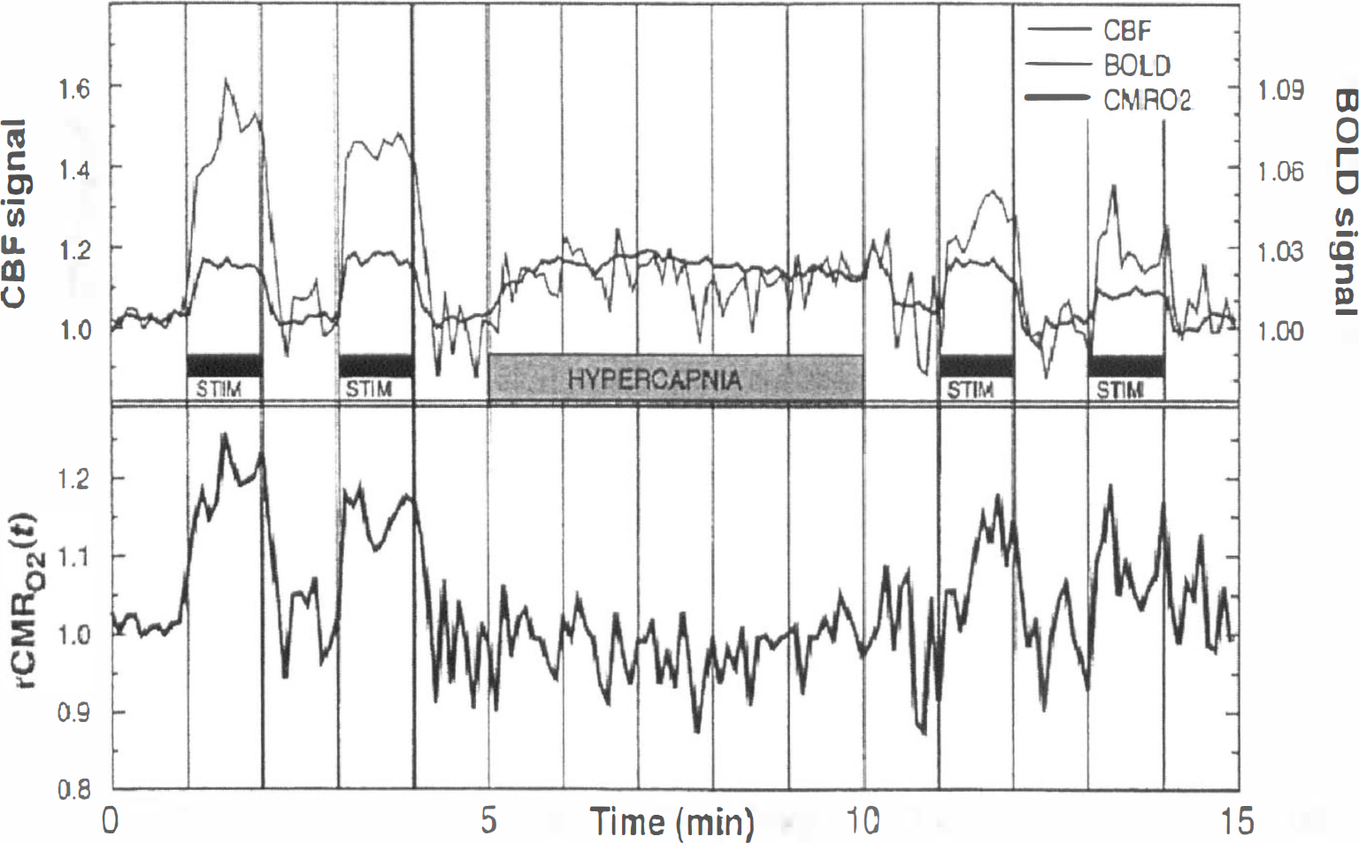
ADVANTAGES AND DISADVANTAGES OF PERFUSION MRI TECHNIQUES
Exogenous versus endogenous contrast agents
Although methods using both exogenous and endogenous contrast agents can be considered as noninvasive (neither requiring ionizing radiation), ASL has the extra benefit of using an endogenous contrast agent. Therefore, multiple measurements can be performed, in principle, without any restriction. Although multiple bolus injections of contrast agent can be performed, the acceptable maximum dose is limited. A lower dose must be administered in multiple measurements, thus reducing the sensitivity of the technique.
Behavior under extreme flow conditions
Although both MRI techniques using exogenous or endogenous contrast agents behave reasonably well in the range of normal CBF values, they have difficulties when dealing with high or low flow. With a low flow, the first obvious limitation is the low SNR of the measurement. This can be improved in the ASL technique by increasing the number of averages (at the expense of increasing the measurement time). On the other hand, in the typical single-bolus DSC studies, because of its dynamic character, averaging is not an option. One possible solution is the use of a larger dose, although the maximum dose is limited (e.g., by Food and Drug Administration regulations). However, SNR is not the only problem when measuring low flows. The second problem is related to the presence of long arrival delays for the arterial blood to the VOI, which may result from collateral circulation in the periphery of stroke regions. Extra delays of up to several seconds can be observed in the ischemic tissue. Although the latest ASL sequences proposed (Alsop and Detre, 1996; Wong et al., 1998a) are less sensitive to differences in transit time (provided an appropriate choice of sequence parameters are chosen), long transit times may make use of the required parameters impractical. In PASL, the transit time insensitivity can be further improved by slice profile optimization (Pell et al., 1998). Another possibility would be to take account of the different transit times, for instance, by measuring them (Zhang et al., 1992; Ye et al., 1997b; Wong et al., 1997; Barbier et al., 1998; Branch et al., 1998), or by using the bolus arrival time information from a DSC experiment. However, this problem is one of the fundamental limitations of the ASL technique for measuring CBF in the presence of long transit time delays. In the case of a long delay, it may be impossible to have tagged signal arriving at the tissue and, therefore, no effect will be observed. There is no simple solution to this problem apart from the use of a higher magnetic field strength with the associated longer T1.
The presence of long bolus arrival times also is a problem in DSC studies. The transit of the bolus from the site of injection (typically a vein) to the VOI can introduce a delay, as well as dispersion (spread of the bolus shape). This dispersion effectively reduces the labeling (bolus sharpness), and, therefore, the dispersion can be thought of as a “relaxation” process (the more spread the bolus, the smaller the observed effect). If one does not account for this delay and dispersion, it may cause an overestimation of MTT and underestimation of CBF (Østergaard et al., 1996a, b , 1999; Schreiber et al., 1998). However, this apparent increase in MTT is not related to the increase caused by true intravoxel dispersion. The main problem is that the DSC model cannot distinguish between dispersion in the feeding vessels (from the place where the AIF was estimated, e.g., MCA, to the VOI) and intravoxel dispersion by tissue microvasculature within the VOI (Østergaard et al., 1999; Schreiber et al., 1998). Although one can account for the dispersion from the site of injection (vein) to the artery where the AIF is estimated, this can not been done for the extra dispersion from the artery to the input of the VOI (where the true AIF should be obtained). This extra dispersion is particularly significant in cases of collateral flow to ischemic areas. To address this problem, Østergaard et al. (1999) have incorporated a mathematical vascular model into the DSC analysis. They show that the vascular model approach is less sensitive to vascular delay and dispersion than the conventional deconvolution approach. Their results are promising, but further validation on many patients with cerebrovascular diseases is needed.
The case of high flows also is problematic for the ASL technique because the assumption of complete exchange is no longer valid (Silva et al., 1997a, b ). If this is not taken into account, the perfusion will be underestimated (since only a fraction of the arterial magnetization is exchanged).
Regional coverage
Both techniques can be used in a multislice protocol, although the maximum number of slices is limited in each case. In DSC-MRI, the coverage is given by a compromise between the number of slices and the time resolution. For a full characterization of the bolus passage, high time resolution is required (the sharper the bolus, the higher the time resolution). For typical repetition time values, a coverage of 10 to 15 slices can be achieved using EPI. Another possibility is the use of three-dimensional acquisitions (Petrella et al., 1997), although with a lower spatial resolution. For the case of ASL, as mentioned in the section on perfusion MRI using spin labeling of arterial water, there are certain limitations to the maximum number of slices. Accurate quantification from about 5 slices typically can be obtained and, in a recent study, up to 10 slices have been acquired using spiral EPI, although with limited spatial resolution (Yang et al., 1998).
CONCLUSION
The demonstration that MRI can be sensitized to detect levels of CBF has generated considerable research activity. As a result, increasingly accurate quantification is possible. Over the last few years, the DSC technique has been used to a greater extent than ASL. This can be explained by the earlier origin of the former technique. In addition, the analysis of DSC-MRI is more straightforward if summary parameters are used. Furthermore, with the advent of EPI in a clinical environment, multislice DSC-MRI has become an immediate option. On the other hand, the original ASL techniques were not possible to extend to multislice (apart from the two-coil case), and it has only recently become a multislice technique. Notice that the only application where the use of ASL has been more commonplace than DSC-MRI is in the field of tMRI. As mentioned before, this is the application where the complete noninvasive character of ASL makes it particularly superior to DSC-MRI.
In conclusion, although certain issues concerning absolute quantification remain to be fully addressed, both perfusion MRI techniques have evolved to be an important tool in research laboratories and clinical units, and they are used in a routine way by an increasing number of centers every day. For clinicians, the high contrast and ease of data acquisition of DSC-MRI make it appealing, whereas for research on brain function, the noninvasive character of ASL with its freely diffusible tracer, blood water, is highly desirable. Both approaches are likely to evolve over the coming years to become faster and more accurate, although which technique will prove to be superior with regard to noninvasive CBF quantification remains to be seen.