Sage Journals: Discover world-class research

Abstract

Cerebral blood flow (CBF) and vascular mean transit time (MTT) can be determined by dynamic susceptibility contrast-enhanced magnetic resonance imaging and deconvolution with an arterial input function. However, deconvolution by a singular value decomposition (SVD) method is sensitive to the tracer delay that often occurs in patients with cerebrovascular disease. We investigated the effect of tracer delay on CBF determined by SVD deconvolution. Simulation study showed that underestimation of CBF due to tracer delay was larger for shorter MTTs. We developed a delay correction method that determines tracer delay by means of least-squares fitting pixel-by-pixel. The corrected CBF was determined by SVD deconvolution after time-shifting of the measured concentration curve. The simulations showed that the corrected CBF was insensitive to tracer delay irrespective of the vascular model, although CBF fluctuation increased slightly. We applied the delay correction to the CBF and MTT images acquired for nine patients with hyperacute stroke and unilateral occlusion of the middle cerebral artery. We found in some patients that the delay correction modulated the contrast of CBF and MTT images. For hyperacute stroke patients, tracer delay correction is essential to obtain reliable perfusion image when SVD deconvolution is used.

Keywords

cerebral blood flow deconvolution dynamic susceptibility contrast-enhanced magnetic resonance imaging singular value decomposition tracer delay

Introduction

Dynamic susceptibility contrast-enhanced magnetic resonance imaging (DSC-MRI) that uses a contrast medium provides brain perfusion images such as cerebral blood flow (CBF), cerebral blood volume (CBV), and vascular mean transit time (MTT) image. In the acute stage of stroke, the perfusion measurement combined with diffusion-weighted imaging is useful in the estimation of the area of tissue at risk for infarction (Baird and Warach, 1998; Schlaug et al, 1999; Sorensen et al, 1999). When an arterial input function (AIF) that corresponds to the contrast medium concentration in the artery can be measured, deconvolution provides measurements of CBF and MTT (Gobbel and Fike, 1994; Rempp et al, 1994; Østergaard et al, 1996a, 1996b; Schreiber et al, 1998). Østergaard et al (1996a) have compared some deconvolution methods by computer simulations, and concluded that singular value decomposition (SVD) deconvolution was most appropriate to estimate CBF. However, estimation of CBF by SVD deconvolution is extremely sensitive to the presence of the arrival delay (Østergaard et al, 1996a; Calamante et al, 2000; Wu et al, 2003b). Calamante et al (2000) found by simulation that several seconds of delay caused underestimation of CBF by a maximum of 50%. For measurement in stroke patients, hemodynamics might be changed dramatically from the normal physiologic conditions, and significant tracer delay may occur in the ischemic brain region. In processing of DSC-MRI data, the AIF is measured with the automated program (Rempp et al, 1994; Murase et al, 2001a; Carroll et al, 2003) or manual selecting of arterial pixels (Østergaard et al, 1996b; Wirestam et al, 2000; Mukherjee et al, 2003) in a large feeding vessel such as the internal carotid artery or middle cerebral artery (MCA), and is applied to the deconvolution for all brain regions. One possible approach to reduce the effect of delay is to use an AIF measured in a large artery near the affected region (Yamada et al, 2002), although this method is not practical for pixel-by-pixel processing. Murase et al (2001b) investigated the relation between the effect of delay and cutoff parameter in SVD and concluded that the optimum could not be determined. Some deconvolution methods that are less sensitive to tracer delay, such as deconvolution based on the maximum likelihood estimation (MLE) method (Vonken et al, 1999) and a modified SVD deconvolution that uses a block-circulant matrix (Wu et al, 2003a), have been proposed. However, a delay correction method for SVD deconvolution is not well established.

We used numerical simulations to develop a delay correction method for CBF determined by SVD deconvolution. Our method determines the tracer arrival delay by means of least-squares fitting pixel-by-pixel. Then, the corrected CBF is determined by SVD deconvolution after time-shifting of the measured concentration curve. To investigate the effect of delay on clinical CBF images, we applied the delay correction to the data for a patient group with hyperacute stroke and compared corrected with uncorrected CBF.

Methods

Theory

Cerebral blood flow, CBV, and MTT measurements by the DSC-MRI are based on indicator-dilution theory (Meier and Zierler, 1954). The tracer concentration as a function of the time after contrast medium bolus injection is as follows:

C_{t} (t) = \frac{1}{k_{h}} C B F C_{a} (t) \otimes R (t)

(1)

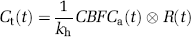
where C_t(t) is the concentration in each pixel, CBF is CBF in mL/min mL unit, C_a(t) is the AIF, R(t) is a residue function which describes a residual probability as a function of the time after tracer arrival, and k_h is a correction factor for the hematocrit difference between a large vessel (h_l) and a capillary (h_s), k_h=(1−h_l)/(1−h_s). The relation between the MR signal intensity and the tracer concentration is described by

S_{t} (t) = S_{t 0} exp (- Δ R_{2}^{*} T E)

(2)

= S_{r 0} exp (- K_{t} C_{t} (t) T E)

(3)

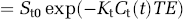
where S_t(t) is the signal intensity, S_t0 is the baseline signal before tracer arrival, ΔR₂* is the change in transverse relaxation rate induced by the contrast medium, TE is the echo time, and K_t is a constant factor relating the tracer concentration with ΔR₂*. An expression for C_t(t) is obtained from equation (3):

C_{t} (t) = - \frac{1}{K_{t} T E} ln (\frac{S_{t} (t)}{S_{t 0}})

(4)

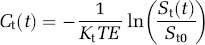
For the artery, an equivalent equation is obtained:

C_{a} (t) = - \frac{1}{K_{a} T E} ln (\frac{S_{a} (t)}{S_{a 0}})

(5)

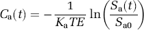
By introducing C_t′(t)=−ln(S_t(t)/S_t0) and C_a′(t)=−ln(S_a(t)/S_a0) as ‘normalized concentrations’ (Smith et al, 2003), the main equation to solve is obtained:

C_{t}^{'} (t) = \frac{K_{t}}{K_{a} K_{h}} C B F C_{a}^{'} (t) \otimes R (t)

(6)

Cerebral blood flow can be determined as the maximum value of the function obtained by SVD deconvolution of equation (6) with the AIF (Østergaard et al, 1996a). In this study, the cutoff level in SVD deconvolution was fixed at 15% of the maximum singular value. Cerebral brain volume is calculated as the ratio of the areas under the tissue curve and the AIF:

C B V = α^{- 1} \int C_{t}^{'} (t) d t / \int C_{a}^{'} (t) d t

(7)

Mean transit time is calculated from CBF and CBV by a central volume principle:

M T T = C B V / C B F

(8)

We used the relative CBF and CBV rather than absolute values and set α=K_t/(K_ak_h) to unity.

Delay Correction

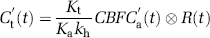
The delay correction scheme is shown in Figure 1. The measured dynamic data in each pixel are fit by the least-squares method and a convolution of the AIF with the exponential function:

Figure 1

Scheme of the delay correction (patient 3). (A) The tissue curve before the maximum concentration in each pixel is fit by least-squares with the AIF and then the arrival delay is determined. In this case, the tissue curve was measured in a pixel near the ischemic core and the delay was 5.0 secs. (B) The delay-corrected tissue curve and AIF. (C) CBF·R(t) (residue function multiplied by CBF) obtained by SVD deconvolution with (solid line) and without (dotted line) the delay correction.

C_{t}^{'} (t) = a C_{a}^{'} (t - d) \otimes exp (- b t)

(9)

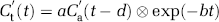
where a and b are free parameters, and d is the delay to be determined (Figure 1A). Only the dynamic data before the concentration peak are fit to determine the delay because the tail part of the data reflects the vasculature rather than the information of tracer arrival timing. The pixel-by-pixel fitting produces a delay image showing the tracer arrival differences between the AIF and each brain tissue. After pixel-by-pixel time-shifting of the measured dynamic data by the estimated delay (Figure 1B), the delay-corrected CBF can be determined as the maximum value of the function obtained by the SVD deconvolution (Figure 1C).

Simulation study

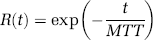
Simulations were performed to investigate the effect of delay on CBF and to test the delay correction method. In the computer simulations, C_t′(t) for a given MTT was calculated from the AIF (C_a′(t)) and an assumed residue function (R(t)). The shape of the AIF measured in an acute stroke patient (patient 3 in the study, Figure 1A) was used for all simulations. To test the versatility of the correction method for various vasculatures, two different vascular models were used for the residue function (Østergaard et al, 1996a). The first was a ‘box-shaped’ model that assumed a vasculature with equal-length vessels having the same MTT:

R (t) = {\begin{array}{l} 1, & 0 \leq t \leq M T T \\ 0, & t > M T T \end{array}

(10)

The second, ‘exponential’ model described the vascular space as a well-mixed compartment:

R (t) = exp (- \frac{t}{M T T})

(11)

The convolution kernel used for the fitting (equation (9)) is identical with the exponential function used for simulations (equation (11)). Therefore, the point in the simulation is whether the method can determine the delay appropriately even for the box-shaped model.

Random noises were added to simulate an actual MR signal (Smith et al, 2003). The signal-to-noise ratio (SNR) of C′(t) was calculated from C′(t) itself and the intrinsic SNR of an MR signal, SNR_S, as follows:

S N R (t) = S N R_{s} C^{'} (t) exp (- C^{'} (t))

(12)

S N R_{s} = S_{t 0} / σ

(13)

where S_t0 and σ are the average and standard deviation of MR signals before tracer arrival. In this study, we set SNR_S=76 (1/SNR_S=1.3%), a typical value for our measurements obtained by gradient echo echo-planar imaging (EPI) with preprocessing by a 3 × 3 uniform filter for a 128 × 128 pixel image. This value was used for all simulations. Some additional simulations with different SNR_S values were performed to examine the noise dependence. In measurements for normal volunteers at our institute, typical normalized concentrations at peak were 1.14 for AIF, 0.44 for gray matter, and 0.15 for white matter. These values corresponded to signal losses (1−S/S₀) of 60%, 36%, and 14%, respectively. These data were used in the simulations for flow levels in gray matter CBF and white matter CBF.

Sixty sequential values of C_t′(t) with a 1-sec interval were generated for the simulations. Cerebral blood flow was determined as the maximum value of the residue function obtained by SVD deconvolution (Østergaard et al, 1996a). The cutoff level was fixed to 15% of the maximum singular value. The effect of delay was simulated by time-shifting of the AIF. In simulation results, CBF was represented as the ratio of measured CBF with the presence of delay to that without delay, CBF_M/CBF_{NO DELAY}. We compared the delay-corrected CBF with the uncorrected CBF. The calculations were repeated 100 times to estimate the effect of noise, and then the average and standard deviation were calculated.

Patient Study

The perfusion study was performed on nine patients with hyperacute ischemic stroke and unilateral occlusion of the MCA confirmed by MR angiography (Table 1). Informed consent was obtained from all the patients or their relatives before the study. All patients were scanned within 6 hours of onset using a 1.5-T whole-body scanner (Magnetom Vision, Siemens Medical System). The perfusion data were obtained with a single-shot gradient-echo EPI (TR=1000 ms, TE=66 ms, flip angle=90°, 23-cm field of view, 5-mm slice thickness) immediately after a bolus injection of 10-mL Gd-DTPA. This contrast medium was injected into the antecubital vein over a period of 3 secs, followed by an injection of 10-ml saline. We obtained 60 images with a 1-sec repetition time in 5 slices. One slice covered the cerebellum and the other 4 slices were in the cerebrum at 0, 12, 24, and 36 mm above and parallel to the anterior commissure–posterior commissure (AC–PC) line. The image matrix size was 128 × 128 pixels. Images were processed with a 3 × 3 uniform filter to reduce the effect of noise. The AIF was measured with a semiautomated method as follows: First, a rectangular region of interest that covered the insular segment in MCA region contralateral to the ischemic side was drawn manually on the second slice (0 mm above the AC–PC line). For each pixel in the rectangular region, the bolus index, defined as the ratio of the peak of C_t′(t) to its time, C_peak′/t_peak, was calculated. AIF was determined by averaging the 5 pixels in which the bolus index was the largest. In addition to the perfusion data, T2-weighted images were measured with a typical turbo spin-echo sequence.

Table 1

Summary of stroke patients

Patient	Age/sex	Time after onset (mins)	Occlusion site
1	68/F	90	rt. MCA
2	80/F	70	lt. MCA
3	65/F	80	rt. MCA
4	74/F	35	lt. MCA
5	69/F	115	lt. MCA
6	64/F	310	rt. MCA
7	75/F	60	lt. MCA
8	60/M	225	rt. MCA
9	75/F	75	rt. MCA

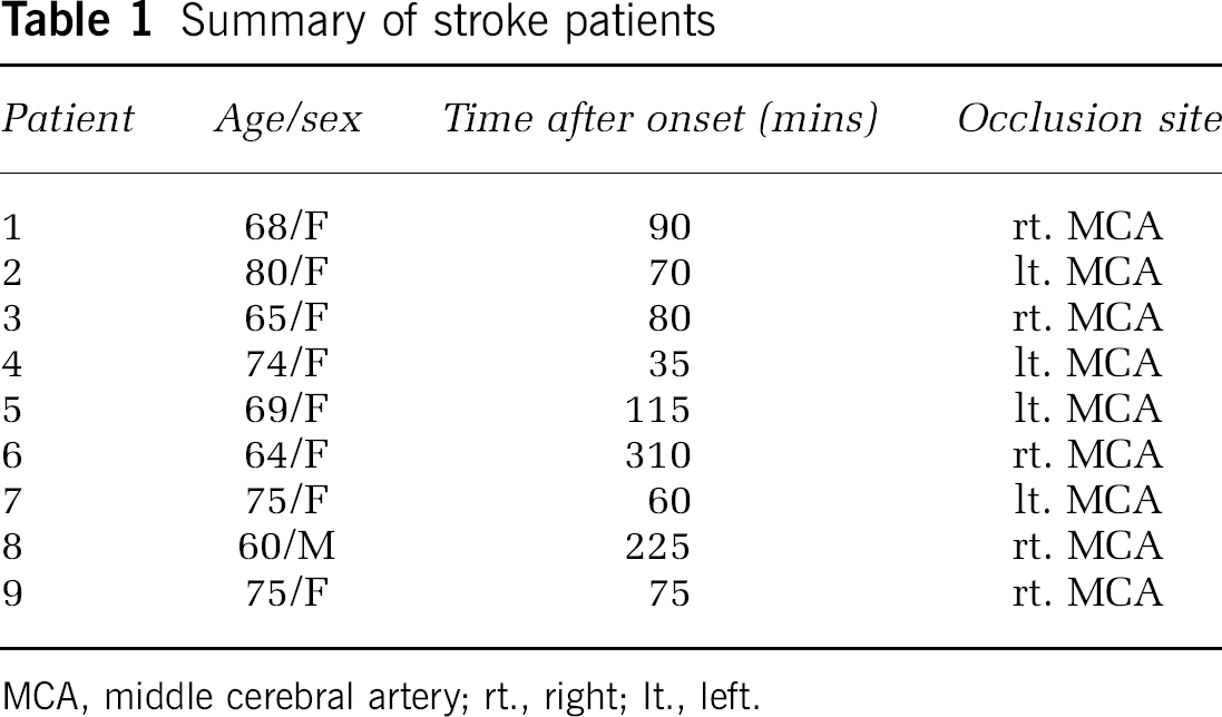
MCA, middle cerebral artery; rt., right; It., left.

Singular value decomposition deconvolution with the measured AIF was performed to generate the CBF image with and without delay correction. Cerebral blood volume and MTT were calculated by equations (7) and (8), respectively. The unit of MTT was the second. The delay correction was not needed for CBV because it is determined by the ratio of the area under the tissue curve to AIF (equation (7)) and is relatively insensitive to the time shift of the dynamic curve. Although an absolute measurement of the AIF is needed for absolute CBF and CBV measurements, a partial volume effect associated with the relatively poor spatial resolution makes it difficult (Calamante et al, 2002). Therefore, for absolute quantification, an additional data processing with a correction or scaling of the estimated AIF is needed. In this study, we calculated relative CBF and CBV values rather than the absolute values: CBF and CBV values were normalized to whole-brain CBF before the delay correction and whole-brain CBV, respectively.

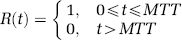
To investigate the effect of delay on CBF images quantitatively, brain image for each patient was divided into three regions according to the degree of perfusion abnormality. The ‘normal’, ‘moderate’, and ‘severe’ regions were defined by the uncorrected MTT value as follows:

‘normal’ region, 0<MTT_i⩽MTT_c+2 secs

‘moderate’ region, MTT_c+2 secs<MTT_i⩽MTT_c+6 secs

‘severe’ region, MTT_c+6 secs<MTT_i

where MTT_i is the uncorrected value in each pixel and MTT_c is an uncorrected normal control value measured in the cerebral cortex on the unaffected side (a 16-mm × 8-mm elliptical region of interest). In the three regions, the averages of CBF with and without delay corrections were calculated and compared. This analysis was performed for the data of the 4th slice (24 mm above the AC–PC line).

Results

Simulation Study

Simulation results for the measured CBF without the delay correction are shown in Figure 2. The measured CBF decreased as the delay increased and then converged to a constant value with oscillation. The amount of CBF underestimation depended on MTT value and was larger for shorter MTTs. For example, 3 secs of delay caused underestimations of 10% (MTT=10 secs) to 40% (MTT=3 secs) for the exponential vascular model and 0% (MTT=10 secs) to 50% (MTT=3 secs) for the box-shaped vascular model. The results were less sensitive to the flow level, but the standard deviations of CBF were larger in the white matter. The CBF underestimation in the presence of delay is illustrated in Figure 3, which shows the residue function obtained by SVD deconvolution for the box-shaped vascular model. The deconvolution could not reproduce the shape of the residue function because the singular values below the cutoff (15% of maximum singular value in the present study) were set to 0 in SVD deconvolution. This resulted in CBF underestimation in the case of a short MTT.

Figure 2

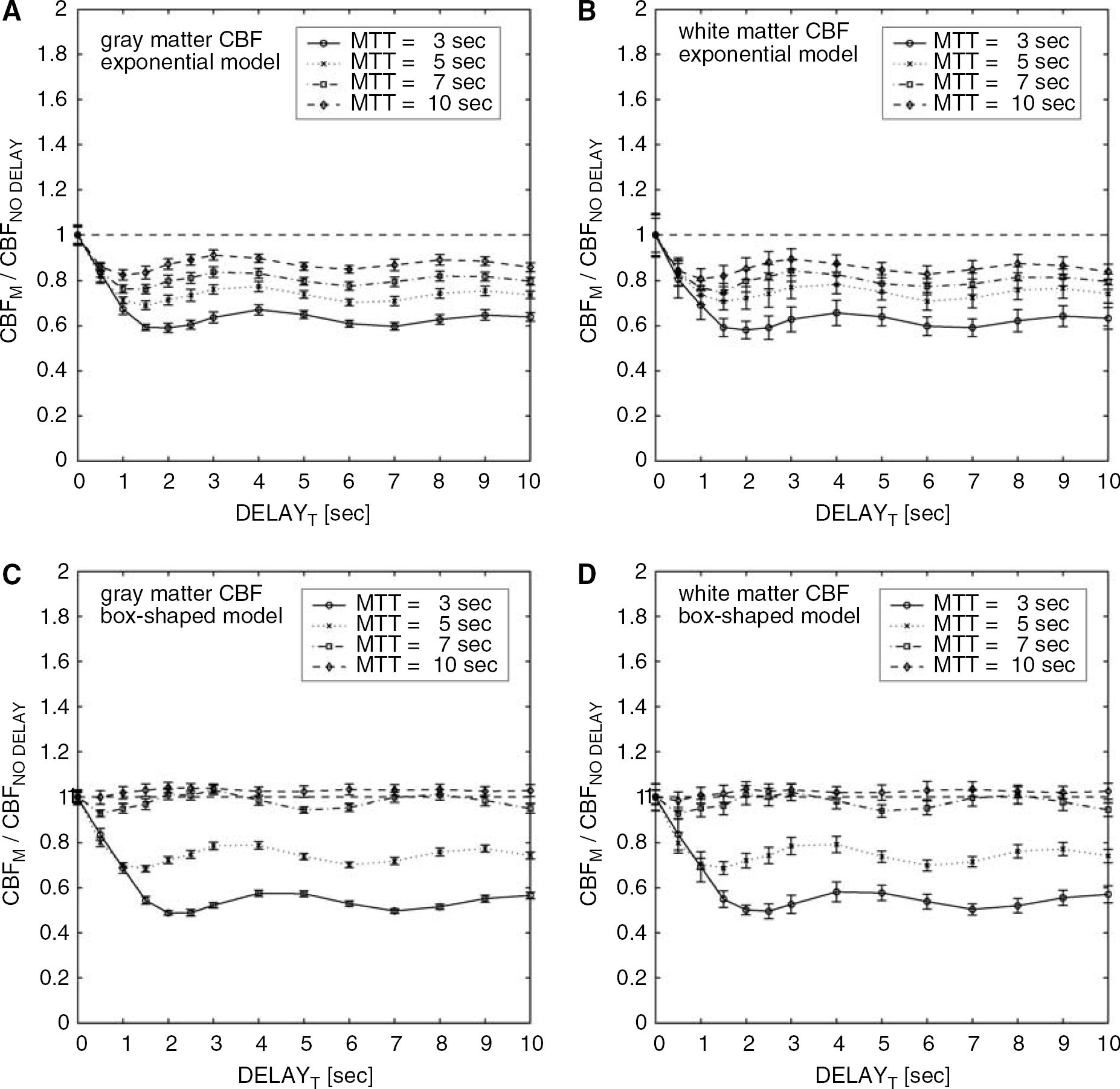
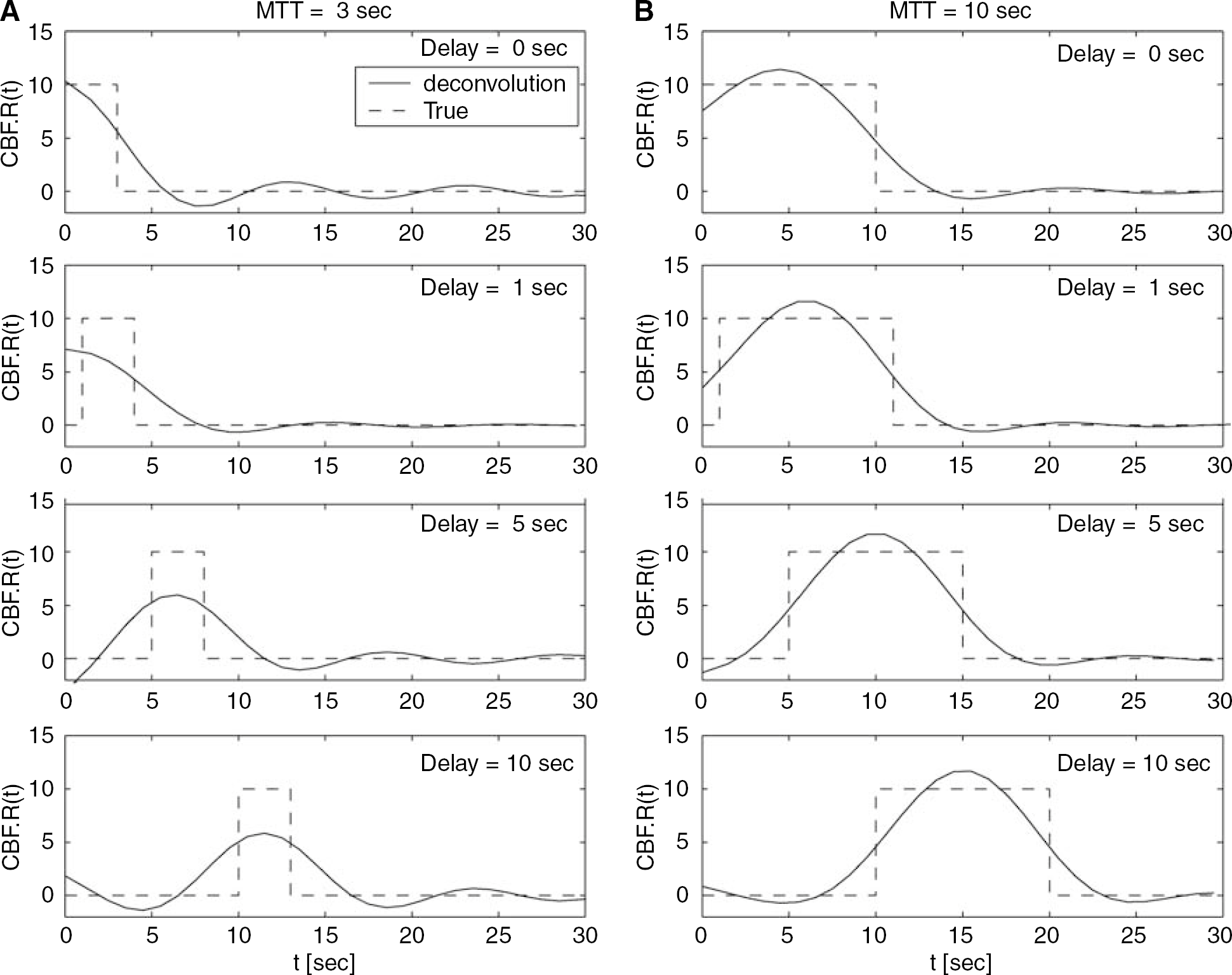
Results of simulations for the measured CBF without the delay correction. The ratio of CBF with the presence of delay to that without delay, CBF_M/CBF_{NO DELAY}, was calculated as a function of tissue delay (DELAY_T) for two flow levels in gray matter (A, C) and white matter CBF (B, D) and for the exponential (A, B) and the box-shaped (C, D) vascular models.

Figure 3

Comparisons between the true residue functions (dotted line) and those obtained by SVD deconvolution (solid line) for various delay conditions (0, 1, 5 and 10 secs). Box-shaped residue functions were assumed with 3-secs (A) and 10-secs (B) MTT. The CBF value is determined from the maximum value of CBF R(t) obtained by the deconvolution. Results show that SVD deconvolution underestimates CBF for a 3-secs MTT because the shape of the residue function is too steep to be recovered by SVD deconvolution with a cutoff of 15% of the maximum singular value.

Comparison of the delay determined by least-squares fitting, DELAY_M, with the true delay, DELAY_T, is shown in Figure 4. The results were less sensitive to the flow level, but the standard deviations were larger for the white matter CBF. The averages of DELAY_M reproduced DELAY_T for both vascular models well. The maximal difference between the averages of DELAY_M and DELAY_T was 0.2 secs for the exponential model and 0.4 secs for the box-shaped model.

Figure 4

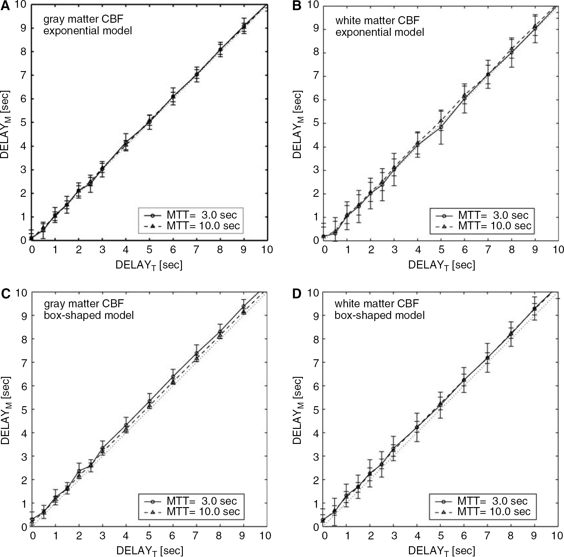
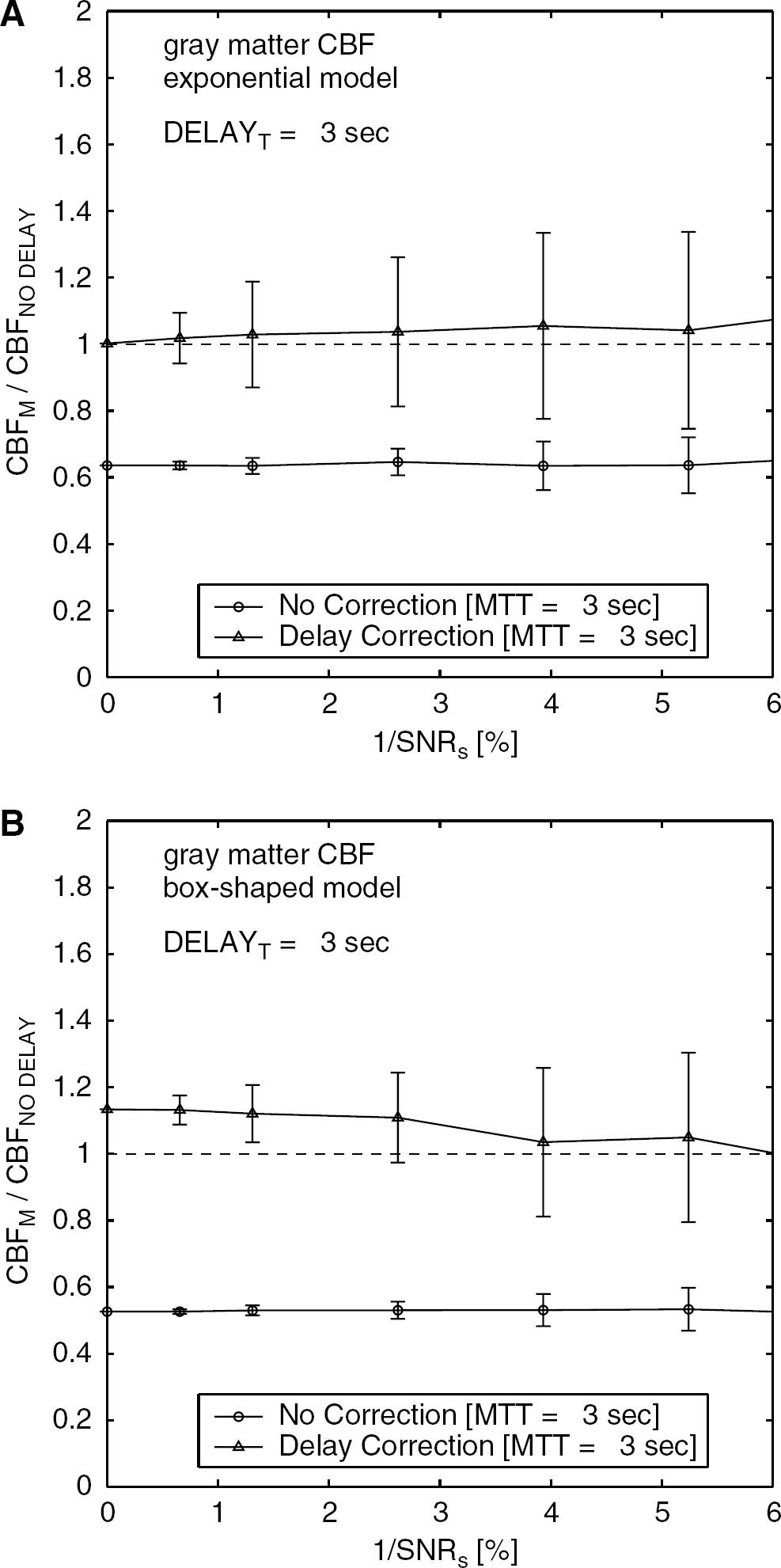
Results of simulations for the delay determined by fitting (DELAY_M) as a function of the true delay (DELAY_T) for two flow levels in gray matter (A, C) and white matter CBF (B, D) and for the exponential (A, B) and box-shaped (C, D) vascular models when the MTT is 3 secs (normal) and 10 secs (prolonged).

Figure 5 (exponential model) and 6 (box-shaped model) show the measured CBF with and without the delay correction. For both of the vascular models, the delay correction resulted in a constant CBF irrespective of the delay. The averages of CBF_M/CBF_{NO DELAY} with the delay correction were between 1.0 and 1.1 for the various delays, the two models, and the two flow levels. However, the correction increased the standard deviations of the measured CBF up to ±25% in the worst case. Although all simulations presented above were performed with 1/SNR_s=1.3%, additional simulations (Figure 7) indicated that the standard deviation of the measured CBF with the delay correction increased as SNR decreased.

Figure 5

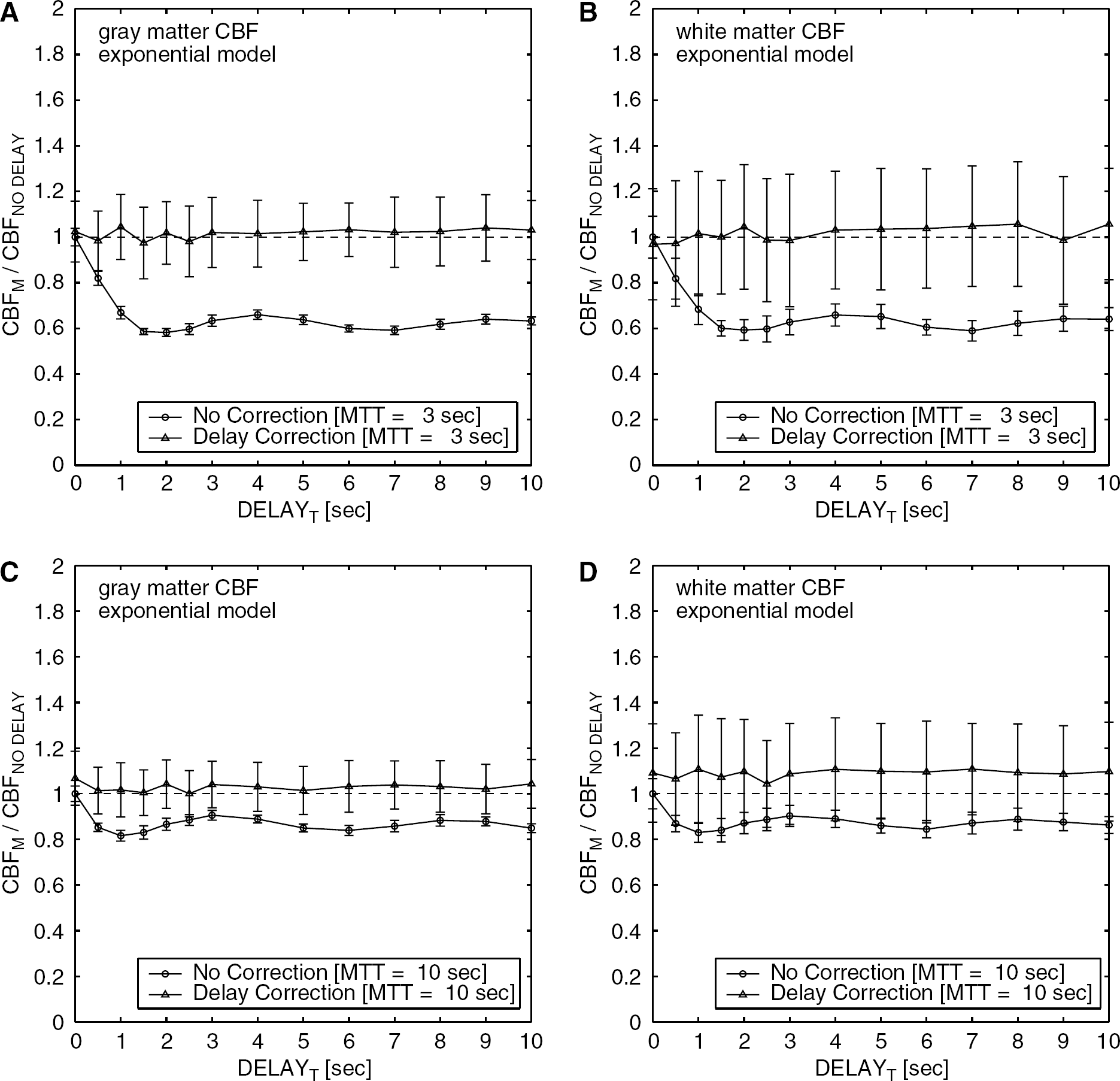
Results of simulations assuming an exponential vascular model for comparison between delay-corrected CBF and uncorrected CBF. The ratio of the measured CBF with the presence of delay to that without delay, CBF_M/CBF_{NO DELAY}, was calculated with (triangle) and without (circle) delay correction. Results for two flow levels in gray matter (A, C) and white matter CBF (B, D) and for 3-secs (A, B) and 10-secs (C, D) values of MTT are presented.

Figure 6

Results of simulations same as those in Figure 5, except that the box-shaped vascular model was assumed. Results for two flow levels in gray matter (A, C) and white matter CBF (B, D) and for 3-secs (A, B) and 10-secs (C, D) MTT are presented.

Figure 7

The simulated ratio of CBF_M/CBF_{NO DELAY} as a function of SNR of baseline signal (SNR_s). Results are for two vascular models: exponential (A) and box-shaped (B).

Patient Study

The tracer delay and the CBF in the three regions are given in Table 2. Examples of the segmented three regions (‘severe’, ‘moderate’, and ‘normal’ region) are shown in Figures 8C and 9C. In all patients, the CBF was smallest in the ‘severe’ region that corresponded to the ischemic core, and was second smallest in the ‘moderate’ region that contained the tissues surrounding the ischemic core, irrespective of the delay correction (Figure 10). In all patients, the delay was largest in the ‘severe’ region and was second largest in the ‘moderate’ region (Figure 11). Among the nine patients, the delay correction increased CBF for eight patients in the ‘severe’ region, for nine patients in the ‘moderate’ region, and for five patients in the ‘normal’ region. In six of nine patients, the CBF increase by the delay correction was larger in the ‘moderate’ region than in the ‘severe’ region.

Figure 8

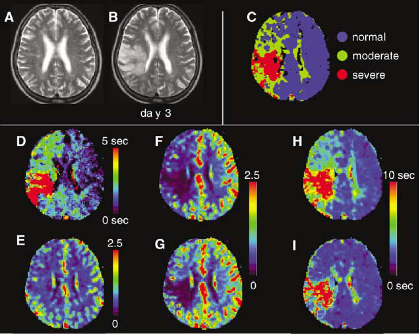
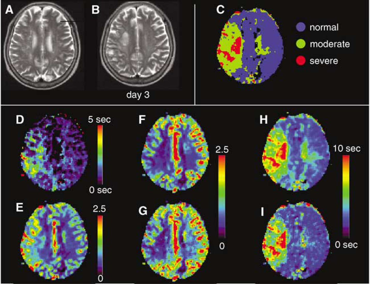
Perfusion images from a 65-year-old woman with hyperacute ischemic stroke and right MCA occlusion 80 mins after onset. (A) T2-weighted image; (B) Three-day follow-up T2-weighted image; (C) segmented brain regions; (D) delay; (E) CBV; (F) uncorrected CBF; (G) corrected CBF; (H) uncorrected MTT; (I) corrected-MTT. MTT is mean transit time.

Figure 9

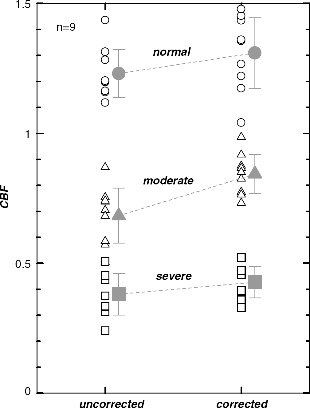
Perfusion images from a 68-year-old woman with hyperacute ischemic stroke and right MCA occlusion 90 mins after onset. (A) T2-weighted image; (B) three-day follow-up T2-weighted image; (C) segmented brain regions; (D) delay; (E) CBV; (F) uncorrected CBF; (G) corrected CBF; (H) uncorrected MTT; (I) corrected-MTT. MTT is mean transit time.

Figure 10

Corrected CBF and uncorrected CBF in the ‘normal’, ‘moderate’, and ‘severe’ regions. Symbols represent the averages for nine patients.

Figure 11

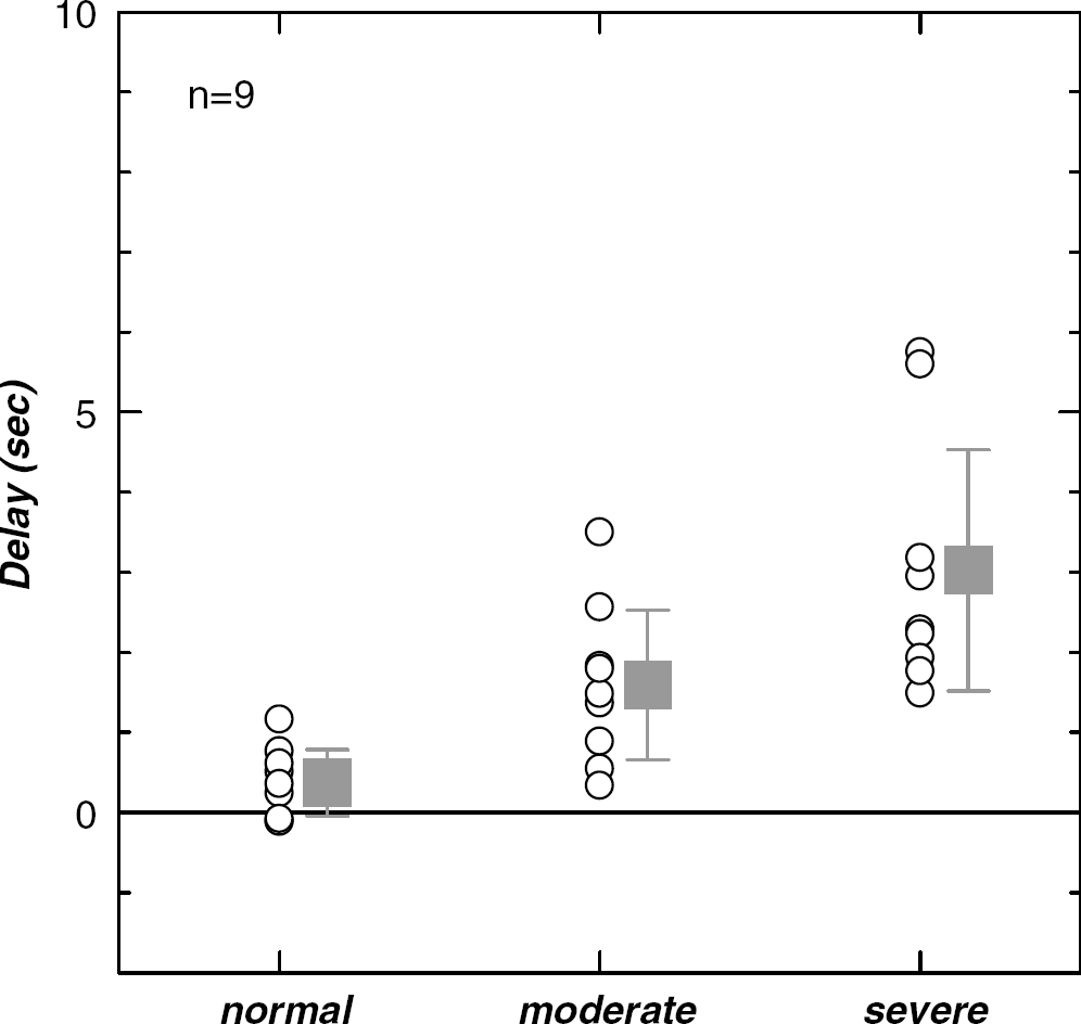
Tracer delays measured in the ‘normal’, ‘moderate’, and ‘severe’ regions. Boxes represent the averages for nine patients.

Table 2

Delay and uncorrected and corrected CBF for three regions

Patient	Delay (sec)			CBF uncorrected			CBF corrected			CBF ratio (Corr./Uncorr.)
	Normal	Moderate	Severe	Normal	Moderate	Severe	Normal	Moderate	Severe	Normal	Moderate	Severe
1	0.51	1.37	1.94	1.28	0.75	0.44	1.45	0.92	0.46	1.13	1.22	1.04
2	−0.11	0.55	2.95	1.20	0.87	0.44	1.17	0.87	0.52	0.98	1.01	1.18
3	1.17	2.57	5.60	1.16	0.50	0.24	1.36	0.85	0.33	1.17	1.69	1.37
4	0.36	1.80	3.18	1.16	0.58	0.37	1.22	0.83	0.47	1.05	1.41	1.26
5	−0.07	0.89	1.49	1.12	0.68	0.45	1.04	0.73	0.46	0.93	1.07	1.01
6	0.61	1.48	1.77	1.20	0.74	0.51	1.48	0.99	0.47	1.23	1.33	0.93
7	0.76	1.83	2.29	1.20	0.57	0.32	1.36	0.77	0.38	1.13	1.35	1.16
8	0.25	3.51	5.76	1.44	0.70	0.31	1.43	0.87	0.40	1.00	1.23	1.26
9	−0.11	0.34	2.24	1.31	0.74	0.33	1.27	0.76	0.36	0.96	1.04	1.07


Mean	0.37	1.59	3.02	1.23	0.68	0.38	1.31	0.84	0.43	1.07	1.26	1.14
s.d.	0.41	0.94	1.51	0.09	0.11	0.08	0.14	0.08	0.06	0.10	0.20	0.13

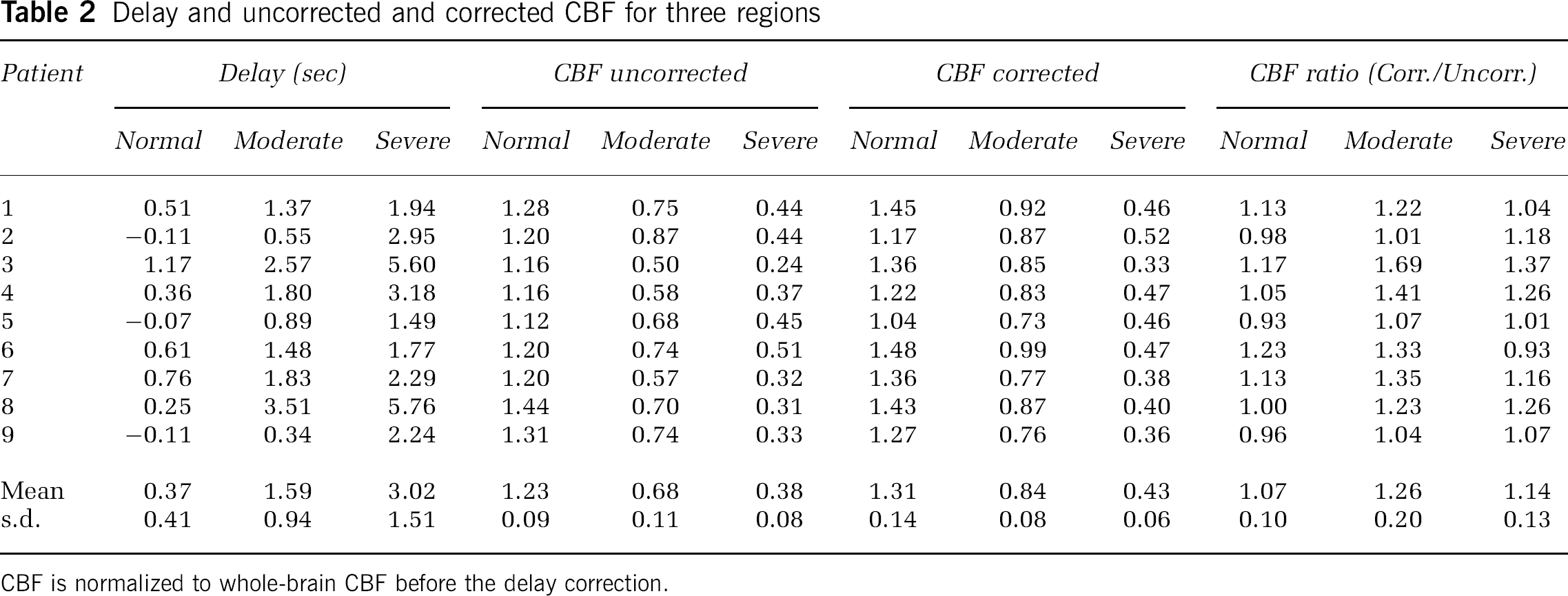
CBF is normalized to whole-brain CBF before the delay correction.

We present the MR images for two representative cases in which the delay correction alters the images dramatically (patient 3) or slightly (patient 1). In patient 3 (Figures 8A to 8I), who was scanned 80 min from stroke onset, significant tracer delays and decreased CBF were observed in a wide area of the right hemisphere. The corrected CBF was markedly larger than the uncorrected CBF for the brain tissues surrounding the ischemic core, but correction had a relatively small effect in the ischemic core. In contrast to CBF, the corrected MTT in the brain tissues surrounding the ischemic core was markedly smaller than the uncorrected MTT and was comparable to the values in the contralateral hemisphere, but the correction had a relatively small effect in the ischemic core. The area estimated by hypoperfusion on the corrected CBF image or prolongation on the corrected MTT image corresponded well to the area of the infarction on follow-up T2-weighted image. In patient 1 (Figures 9A to 9I), who was scanned 90 min after stroke onset, a decreased CBF and prolonged MTT were observed together with tracer delays in the right hemisphere. The delay correction increased CBF and decreased MTT slightly, although the alterations of the CBF and MTT images by the delay correction were not so prominent. In addition to the ischemic brain regions, the delay correction affected CBF and MTT in the cerebral cortex of posterior cerebral artery (PCA) territory and white matter (centrum semiovale of the contralateral hemisphere) where the influence of the MCA occlusion was not supposed to be so strong. This finding was observed in all patients, but the degree of impact varied with patient.

Discussion

Simulation Study

The simulations showed that the delay correction could remove the CBF underestimation caused by SVD deconvolution (Figures 5 and 6). The amounts of CBF underestimation determined by the simulations were similar to those found by other studies (Calamante et al, 2000; Wu et al, 2003b). The results of present simulation emphasized the importance of the delay correction for the short-MTT case. The amount of CBF underestimation depended on the MTT value as well as the delay, and this dependence became stronger with shorter MTT. Large delays do not necessarily cause a large CBF underestimation, and small delays of a few seconds may cause large errors when the MTT is as short as 3 to 5 secs.

The exponential and box-shaped vascular models used in the simulations have an extreme vascular structure and are used frequently in simulation studies (Østergaard et al, 1996a; Calamante et al, 2000; Murase et al, 2001b; Wu et al, 2003a). Our method determined delay values for both vascular models successfully (Figure 4). As a result, SVD deconvolution after time shifting by the fitted delay gave the constant CBF irrespective of the vascular model (Figures 5 and 6). A drawback of the method is that the correction increases the fluctuations of the measured CBF. Apart from the delay correction, deconvolution is intrinsically sensitive to the noise. Cerebral blood flow fluctuations arose from the errors of the fitted delay, were intensified through SVD deconvolution, and increased as the SNR of the MR signal decreased (Figure 7). However, deterioration of the image quality in corrected CBF and corrected MTT was not so conspicuous when preprocessing with a 3 × 3 uniform filter for the raw images and cutoff of small singular values (15% of maximum singular value) in SVD deconvolution were performed (Figures 8 and 9).

Patient Study

The amount of CBF underestimation in the three segmented regions differed (Table 2): the delay correction changed the contrast of the CBF image. In six of nine patients, the CBF increase by the delay correction was largest in the tissues surrounding the ischemic core (‘moderate’ region) even though maximal tracer delay was in the ischemic core (‘severe’ region). This occurred because the MTT around the ischemic core was not as prolonged as that in the ischemic core, and is consistent with simulation result that showed larger effects of delay for shorter MTTs. Therefore, the delay correction has a special impact in application to hyperacute stroke to depict tissue at risk of infarction located around the ischemic core (Schlaug et al, 1999; Sorensen et al, 1999). In patient 3 (Figure 8), the area of abnormal perfusion defined by the corrected CBF and MTT images was clearly smaller than that defined by the uncorrected images. This result shows the importance of the delay correction for the hyperacute stroke patient because the correction may affect the estimation of the diffusion–perfusion mismatch area (Schlaug et al, 1999; Sorensen et al, 1999). However, it is still uncertain whether the delay-corrected CBF and MTT images accurately predict the clinical outcome. A further study on the diffusion–perfusion mismatch and follow-up about the effect of delay will be needed.

Our method generates delay images (Figures 8D and 9D) by least-squares fitting. The delay image by itself has useful information about brain circulation. The delay value is the difference between the tracer arrival time in each pixel and the AIF, whereas the MTT value corresponds to the time needed to pass through the capillary in each pixel. The abnormal region of the delay image differed largely from that of MTT (corrected) image for patient 3 (Figure 8). Wu et al (2003a) calculated the delay image from the residue functions obtained with modified SVD deconvolution using block-circulant matrix, and they proposed the concept of an index of disturbed hemodynamics. In addition to the CBV, CBF, and MTT images, the use of delay image will be helpful in investigating the cerebral circulation of hyperacute stroke patient.

Limitations

Our study accounted only for the effect of delay in SVD deconvolution, although dispersion effects are expected to occur simultaneously in the ischemic brain region. Therefore, delay-corrected CBF may still be underestimated because of the dispersion effect. The correction for the dispersion effect is intrinsically difficult because the dispersion effect and MTT prolongation in the vessel are not distinguishable (Calamante et al, 2000). One approach to this problem is to include the dispersion effect in the vascular model (Østergaard et al, 1999, 2000), although the adequacy of the assumed model for various stroke patients should be validated. To measure CBF, especially for severely ischemic tissues, a method to correct for the effects of delay and dispersion simultaneously will be needed.

A standard method for AIF determination has not been established, although some proposals have been made (Rempp et al, 1994; Murase et al, 2001a; Carroll et al, 2003). We applied the semiautomated method using the bolus index (C_peak′/t_peak) and successfully measured the AIF in the contralateral MCA region for all patients. When the AIF was measured in the region affected by vascular occlusion or stenosis, the effects of delay and dispersion appeared in the AIF (Wu et al, 2003a; Yamada et al, 2002; Mukherjee et al, 2003). Our method can automatically account for the delay in the AIF because the delay determined by fitting has a negative value for the delayed AIF. In the present study, the delays in the ‘normal’ region were positive in 6 of 9 patients and were negative in 3 of 9 patients with almost zero values (−0.11, −0.07, and −0.11 secs). This suggests that the AIF rises earlier than any tissue curve in the brain and supports the validity of the AIF measurement by our method for hyperacute stroke patients.

We calculated relative CBF and CBV values instead of absolute values because some problems of scaling have not yet been solved (Kiselev, 2001), and because of the partial volume effect for the AIF measurement (Calamante et al, 2002; van Osch et al, 2001). K_t and K_a are the constant factors relating the contrast medium concentration with ΔR₂* for brain tissues and the artery, and they depend on factors such as sequence type (gradient-echo or spin-echo EPI), the tracer concentration, and the vascular structure (Fisel et al, 1991; Boxerman et al, 1995; Kiselev, 2001). The K_t for tissues will differ from the K_a for AIF (Kiselev, 2001), and values for pathologic brain tissues may differ from those for normal tissues. These are fundamental problems for both absolute and relative CBF measurements in DSC-MRI study, and warrant further examination.

In conclusion, we have three major findings. First, the amount of CBF underestimation caused by the tracer delay is larger for tissues with short MTTs when SVD deconvolution is used. Second, the delay correction successfully removes the CBF underestimation irrespective of the vascular model. Finally, the delay correction is important for application to the hyperacute stroke because it modulates the contrast of perfusion images (CBF and MTT) and may affect the estimate of the diffusion–perfusion mismatch area.

References

Baird

Warach

(1998) Magnetic resonance imaging of acute stroke. J Cereb Blood Flow Metab 18:583–609

Boxerman

Hamberg

Rosen

Weisskoff

(1995) MR contrast due tointravascular magnetic susceptibility perturbations. Magn Reson Med 34:555–66

Calamante

Gadian

Connelly

(2000) Delay and dispersion effects in dynamic susceptibility contrast MRI: Simulations using singular value decomposition. Magn Reson Med 44:466–73

Calamante

Gadian

Connelly

(2002) Quantification of perfusion using bolus tracking magnetic resonance imaging in stroke: Assumptions, limitations, and potentials for clinical use. Stroke 33:1146–51

Carroll

Rowley

Haughton

(2003) Automatic calculation of the arterial input function for cerebral perfusion imaging with MR imaging. Radiology 227:593–600

Fisel

Ackerman

Buxton

Garrido

Belliveau

Rosen

Brady

(1991) MR contrast due tomicroscopically heterogeneous magnetic susceptibility: Numerical simulations and application to cerebral physiology. Magn Reson Med 17:336–47

Gobbel

Fike

(1994) A deconvolution method for evaluating indicator-dilution curves. Phys Med Biol 39:1833–54

Kiselev

(2001) On the theoretical basis of perfusion measurements by dynamic susceptibility contrast MRI. Magn Reson Med 46:1113–22

Meier

Zierler

(1954) On the theoryof the indicator-dilution method for measurement of blood flow and volume. J Appl Physiol 6:731–44

10.

Mukherjee

Kang

Videen

McKinstry

Powers

Derdeyn

(2003) Measurement of cerebral blood flow in chroniccarotid occlusive disease: Comparison of dynamic susceptibility contrast perfusion MR imaging with positron emission tomography. Am J Neuroradiol 24:862–71

11.

Murase

Kikuchi

Miki

Shimizu

Ikezoe

(2001a) Determination of arterial input function using fuzzy clustering for quantification of cerebral blood flow with dynamic susceptibility contrast enhanced MR imaging. J Magn Reson Imaging 13:797–806

12.

Murase

Shinohara

Yamazaki

(2001b) Accuracy of deconvolution analysis based on singular value decomposition for quantification of cerebral blood flow using dynamic susceptibility contrast-enhanced magnetic resonance imaging. Phys Med Biol 46: 3147–59

13.

Østergaard

Weisskoff

Chesler

Gyldensted

Rosen

(1996a) High resolution measurement of cerebral blood flow using intravascular tracer bolus passages. Part I: Mathematical approach and statistical analysis. Magn Reson Med 36:715–25

14.

Østergaard

Sorensen

Kwong

Weisskoff

Gyldensted

Rosen

(1996b) High resolution measurement of cerebral blood flow using intravascular tracer bolus passages. Part II: Experimental comparison and preliminary results. Magn Reson Med 36:726–36

15.

Østergaard

Chesler

Weisskoff

Sorensen

Rosen

(1999) Modeling cerebral blood flow and flow heterogeneity from magnetic resonance residue data. J Cereb Blood Flow Metab 19:690–9

16.

Østergaard

Sorensen

Chesler

Weisskoff

Koroshetz

Gyldensted

Rosen

(2000) Combined diffusion-weighted and perfusion-weighted flow heterogeneity magnetic resonance imaging in acute stroke. Stroke 31:1097–103

17.

Rempp

Brix

Wenz

Becker

Giickel

Lorenz

(1994) Quantification of regional cerebral blood flow and volume with dynamic susceptibility contrast-enhanced MR imaging. Radiology 193:637–41

18.

Schlaug

Benfield

Baird

Siewert

Lovblad

Parker

Edelman

Warach

(1999) The ischemic penumbra: Operationally defined by diffusion and perfusion MRI. Neurology 53:1528–37

19.

Schreiber

Giickel

Stritzke

Schmiedek

Schwartz

Brix

(1998) Cerebral blood flow and cerebrovascular reserve capacity: Estimation by dynamic magnetic resonance imaging. J Cereb Blood Flow Metab 18:1143–56

20.

Smith

Frayne

(2003) Signal-to-noise ratio effects in quantitative cerebral perfusion using dynamic susceptibility contrast agents. Magn Reson Med 49:122–8

21.

Sorensen

Copen

Østergaard

Buonanno

Gonzalez

Rordorf

Rosen

Schwamm

Weisskoff

Koroshetz

(1999) Hyperacute stroke: Simultaneous measurement of relative cerebral blood volume, relative cerebral blood flow, and mean tissue transit time. Radiology 210:519–27

22.

van Osch

Vonken

Bakker

Viergever

(2001) Correcting partial volume artifacts of the arterial input function in quantitative cerebral perfusion MRI. Magn Reson Med 45:477–85

23.

Vonken

Beekman

Bakker

Viergever

(1999) Maximum likelihood estimation of cerebral blood flow in dynamic susceptibility contrast MRI. Magn Reson Med 41:343–50

24.

Wirestam

Andersson

Østergaard

Boiling

Aunola

Lindgren

Geijer

Holtås

Ståhlberg

(2000) Assessment of regional cerebral blood flow by dynamic susceptibility contrast MRI using different deconvolution techniques. Magn Reson Med 43:691–700

25.

Østergaard

Weisskoff

Benner

Rosen

Sorensen

(2003a) Tracer arrival timing-insensitive technique for estimating flow in MR perfusion-weighted imaging using singular value decomposition with a block-circulant deconvolution matrix. Magn Reson Med 50:164–74

26.

Østergaard

Koroshetz

Schwamm

O'Donnell

Schaefer

Rosen

Weisskoff

Sorensen

(2003b) Effects of tracer arrival time on flow estimates in MR perfusion-weighted imaging. Magn Reson Med 50:856–64

27.

Yamada

Gonzalez

Bakker

Østergaard

Copen

Weisskoff

Rosen

Yagi

Nishimura

Sorensen

(2002) Magnetic resonance perfusion-weighted imaging of acute cerebral infarction: Effect of the calculation methods and underlying vasculopathy. Stroke 33:87–94

Tracer Delay Correction of Cerebral Blood Flow with Dynamic Susceptibility Contrast-Enhanced MRI

Abstract

Keywords

Introduction

Methods

Theory

Delay Correction

Simulation study

Patient Study

Results

Simulation Study

Patient Study

Discussion

Simulation Study

Patient Study

Limitations

References