
Abstract
This work compares equilibrium to kinetic analysis of positron emission tomography data for the assessment of vesicular monoamine transporter (VMAT2) binding density using (+)-α-[11C]dihydrotetrabenazine ((+)-α-[11C]DTBZ). Studies were performed for 80 minutes after intravenous administration of 18 ± 1 mCi (+)-α-[11C]DTBZ on 9 young control subjects, 20 to 45 years of age. A 9-mCi bolus was injected over the first minute of the study, whereas the remaining 9 mCi were infused at a constant rate over the following 79 minutes. Steady-state was reached in both blood and brain by approximately 30 minutes after initiation of the study. Nonlinear least-squares analysis using two- and three-compartment models, weighted integral analysis using a two-compartment configuration, and Logan plot analysis all yielded kinetic estimates of the total tissue distribution volume, DVtot(kin). These results were compared with equilibrium distribution volume estimates, DVtot(eq), calculated from the tissue to metabolite corrected arterial plasma concentration ratio after 30 minutes. Kinetic modeling results from this study were in close agreement with prior bolus-injection (+)-α-[11C]DTBZ studies. In the current study, coefficients of variation in DVtot(kin) (19% to 23% across regions) and DVtot(eq) (18% to 22%) were nearly identical. Equilibrium estimates of DVtot were slightly lower than kinetic estimates, averaging 5% ± 9% lower (P = 0.04, paired t test) in regions of high binding density (caudate and putamen), but only 2% ± 6% (P = 0.09) in lower binding density regions (cortex, thalamus, cerebellum). DVtot(eq) estimates, however, still correlated highly with DVtot(kin) estimates (r = 0.977−0.989). Steady-state conditions can be achieved in both tissue and blood by 30 minutes, and the tissue-to-blood ratios of (+)-α-[11C]DTBZ at equilibrium yield DVtot(eq) measures that are in close agreement with DVtot(kin) estimates. Thus, a simple, easily tolerated protocol using a loading bolus followed by continuous infusion can provide excellent measures of VMAT2 binding.
Keywords
This study assesses the capabilities of using (+)-α-[11C]dihydrotetrabenazine ((+)-α-[11C]DTBZ) and an equilibrium positron emission tomography (PET) protocol for estimating binding to the vesicular monoamine transporter (VMAT2) in the human brain. The VMAT2 binding site is a specific protein located exclusively in the membranes of presynaptic vesicles of monoaminergic neurons (Henry and Scherman, 1989). Radioligands for noninvasive in vivo imaging of VMAT2 binding sites, and hence markers of nigrostriatal neurons, have been developed in our laboratory. Initially (±)-[11C]tetrabenazine (DaSilva and Kilbourn, 1992) was proposed; however, one of the labeled metabolites of that radioligand is (±)-dihydrotetrabenazine, which also crosses the blood-brain barrier and binds to VMAT2 sites, and thus the ability to model (±)-[11C]tetrabenazine kinetics was compromised. Subsequently, (±)-[11C]methoxytetrabenazine (Vander Borght et al., 1995b; Kilbourn, 1994) and (±)-[11C]dihydrotetrabenazine (Koeppe et al., 1995), two radioligands that do not form lipophilic metabolites, have been developed and used for human imaging. Studies have demonstrated that in vivo regional binding of these radioligands correlates with the known distribution of VMAT2 in rodent brain (Kilbourn, 1994; Kilbourn et al., 1995), and that a linear relation exists between the level of in vitro striatal radioligand binding to VMAT2 and the extent of nigral injury in 6-hydroxydopamine–lesioned rats (Vander Borght et al., 1995b). The α-DTBZ exhibits high-affinity binding only to VMAT2, and animal studies have shown a lack of regulation of this transporter by repeated or chronic dopaminergic or cholinergic drug treatments (Naudon et al., 1994, Vander Borght et al., 1995a; Wilson et al., 1996). Although α-DTBZ binding is not specific to dopaminergic nerve terminals, since the radioligand binds to the vesicular transporter common for all monoaminergic neurons, the PET signal measured in the striatum largely represents storage vesicles in the predominant (over 95%) dopaminergic terminals (Kish et al., 1992).
In this work, we describe methods of analysis of PET studies with (+)-α-[11C]dihydrotetrabenazine for quantifying levels of binding to the vesicular monoamine transporter. Preliminary studies used a racemic mixture of the radioligand (±)-α-[11C]DTBZ (Koeppe et al., 1995; Frey et al., 1996; Gilman et al., 1996). However, the (−)-isomer has an extremely low affinity (about 2 μmol/L) for the VMAT2 binding site (Kilbourn et al., 1995), and thus the binding is almost exclusively nonspecific, adding noise but no signal to the measure. Separation of the isomers allows administration of the active isomer (+)-α-[11C]DTBZ (Ki = 0.97 ± 0.48 nmol/L; Kilbourn et al., 1995) alone, substantially increasing the signal to background of the VMAT2 binding measures. Dynamic PET studies in normal volunteers using bolus injections of (+)-α-[11C]DTBZ have been analyzed using a variety of compartmental model configurations and parameter estimation schemes (Koeppe et al., 1996).
Here we present a comparison of an equilibrium analysis of (+)-α-[11C]DTBZ with the kinetic analysis methods reported by Koeppe and coworkers (1996) for the estimation of a VMAT2 binding density index after a single radioligand injection. The kinetic approach requires about an hour of dynamic imaging as well as arterial plasma and metabolite analysis throughout the entire study. An equilibrium or steady-state approach requires acquisition of only a few scans and analysis of only a few blood samples after equilibrium conditions are achieved (about 30 minutes), and thus a considerably simpler and better tolerated protocol can be used. In this study, a more complex data acquisition protocol was used so that both kinetic and equilibrium analyses could be evaluated. However, equilibrium analysis by itself requires only about 30 minutes of imaging and two or three blood samples.
Equilibrium approaches have been proposed and used extensively for tracers that bind reversibly and equilibrate relatively rapidly, such as [11C]raclopride (Farde et al., 1986, 1987, Minoshima et al., 1994), [11C]flumazenil (Persson et al., 1985, 1989; Shinotoh et al., 1986, 1989; Pappata et al., 1988, Frey et al., 1993), and [18F]cyclofoxy (Kawai et al., 1991). Some of these have used continuous-infusion protocols to ensure that true equilibrium conditions between arterial plasma and brain are established (Kawai et al., 1991; Frey et al., 1993; Minoshima et al., 1994), whereas the others are pseudoequilibrium approaches, where a bolus injection is given and scanning is performed under conditions that may approach, but do not reach, true equilibrium. To achieve equilibrium as rapidly as possible, we determined an infusion protocol consisting of a partial bolus to “load” the tissue, followed by continuous administration of the remainder of the dose to achieve and maintain steady-state conditions. In addition, we were interested in evaluating the measured uncertainties in the distribution volume estimates to see whether the simpler calculation afforded by the equilibrium approach provides more stable binding estimates than do the kinetic approaches.
METHODS
Nine young normal volunteers, aged 20 to 45 years, were studied after administration of 666 ± 37 MBq (18 ± 1 mCi) of (+)-α-[11C]DTBZ. A dose of 333 MBq (9 mCi) was administered by intravenous bolus injection over the first minute of the study, whereas the remaining 333 MBq were continuously infused over the remaining 79 minutes of the study. The 50:50 fractionating between bolus and infusion portions of the dose was based on calculations of the clearance rate from plasma from previous bolus studies (Koeppe et al., 1996; see Discussion). No-carrier-added (+)-[11C]DTBZ (250 to 1000 Ci/mmol at time of injection) was prepared, as reported by Jewett and others (1997). A sequence of 17 PET scans (4 × 30 seconds, 3 × 1 minute, 2 × 2.5 minutes, 2 × 5 minutes, 6 × 10 minutes) was acquired in two-dimensional mode on a Siemens/CTI ECAT EXACT-47 scanner (Knoxville, TN) for 80 minutes after injection. Data were reconstructed using a Hanning filter with a cutoff of 0.5 cycles/projection ray, achieving a reconstructed resolution of about 9 mm full-width at half-maximum. Calculated attenuation correction was performed on all data sets.
Blood samples were withdrawn using a radial artery catheter at 10-second intervals for the first 2 minutes and then at progressively longer intervals for the remainder of the study. Plasma was separated from red cells by centrifugation and counted in a Nal well-counter. The plasma radioactivity time course was corrected for radiolabeled metabolites using a rapid Sep-Pak C18 cartridge chromatographic technique similar to that previously reported for scopolamine and flumazenil (Frey et al., 1991; 1992). The samples at 1, 2, and 3 minutes and at all later times (13 in all) were analyzed for metabolites. Aliquots of 0.5 mL of plasma were added to tubes containing and 0.6 mL of a solution of [3H]DTBZ (0.002 mCi) in phosphate-buffered saline. After application to Sep-Pak C18 columns, samples were first washed with 9 mL of a 65:35 mixture of phosphate-buffered saline–ethanol. This fraction contained all metabolites and a portion of the authentic DTBZ. The remainder of the unmetabolized fraction then was eluted from the column with 5 mL of ethanol. Both samples were assayed for 11C activity in the well counter, and then after decay of 11C, assayed for 3H by liquid scintillation counting. The fractionating of [3H]DTBZ (100% authentic) was used to correct for the portion of authentic [11C]DTBZ eluted in the first wash. Metabolite fractions of the samples not analyzed for metabolites were estimated by linear interpolation. Previous studies reported by Frey and colleagues (1996) showed no measurable levels of DTBZ metabolites in the rat brain, even at 80 minutes after injection.
Radioactive fiducial markers were used to correct for patient motion that occurred throughout the study. Molecular sieve beads (1- to 2-mm diameter) were placed at three points on the patient's scalp before the study. Approximately 1 μL of the [11C]DTBZ preparation was pipetted onto each bead at an activity of about 2 μCi per bead. Bead locations defined on a single base frame (frame 10; 10 to 15 minutes after injection) were used for reorientation of the other frames of the study as described by Koeppe and colleagues (1991).
Volumes-of-interest were created on the base frame and applied to the entire dynamic sequence generating time–activity curves for the different brain structures. Regions analyzed included caudate nucleus, putamen, frontal cortex, thalamus, and cerebellar hemispheres. Left and right hemisphere regions were analyzed separately then averaged within each subject before calculation of group means and standard deviations. No significant hemispheric differences were detected.
Dynamic studies were acquired for comparing equilibrium and kinetic analysis techniques in the same set of PET studies. In addition, we compared results of the kinetic analysis from this constant infusion study to those from our previously reported study (Koeppe et al., 1996), which used bolus administrations. This was to assure that changes in input function shape did not affect our ability to estimate model parameters in a dynamic study.
Equilibrium analysis
Estimates of DVtot(eq) were obtained by dividing the concentration of (+)-α-[11C]DTBZ in tissue (measured with PET) by the metabolite-corrected arterial plasma concentration averaged over the portion of the study after equilibrium conditions were achieved: DVtot(eq) = CPET/Cp. For calculation purposes, CPET and Cp were assumed to be constant over the entire “equilibrium” period and averaged over time before calculating their ratio. Both tissue and blood data remained nearly constant 30 minutes after administration, and hence data after 30 minutes were used in calculation of DVtot(eq). Five 10-minute scans were acquired between 30 and 80 minutes after the initiation of tracer administration. Plasma samples were withdrawn every 10 minutes throughout this period to determine the level of authentic (+)-α-[11C]DTBZ. Calculations were performed using two time intervals: 30 to 60 minutes and 30 to 80 minutes. The final 20 minutes of scanning is more certain to be acquired during steady-state conditions, although the 20-minute physical half-life of 11C limits the statistical quality of these later data.
Kinetic analysis
Four separate kinetic analyses were performed on the dynamic data as described by Koeppe and others (1996). In this previous work, it was determined that DVtot provided the most reliable index of VMAT2 density. Nonlinear least-squares analysis using the Marquardt algorithm (Bevington, 1969) was performed with both two- and three-compartment model configurations on the volumes-of-interest–generated time activity data to estimate DVtot. For the two-compartment configuration, K1, DVtot, and CBV were estimated, whereas for the three-compartment configuration, K1, DVf+ns, k3, k4, and CBV were estimated (for details, see Koeppe et al., 1996). Two pixel-by-pixel analyses also were performed on the dynamic data sets: a two-parameter weighted integral analysis (Alpert et al., 1984) producing functional images of ligand delivery (K1) and binding (DVtot(kin)), and a graphic analysis for reversible ligands (Logan et al., 1990) also calculating DVtot(kin) (from data 10 minutes and later) and an approximation for K1 (using the entire data set). Again, further details of the implementation of these methods are given in Koeppe and others (1996). After creation of K1 and DVtot(kin) images for both the weighted integral and Logan plot methods, the volumes-of-interest defined for nonlinear least-squares analysis were applied to the functional images to obtain regional parameter estimates. As with the equilibrium analysis, data over two different scan durations were analyzed: 0 to 60 minutes, and 0 to 80 minutes. Estimates from each of the kinetic methods (DVtot(kin)) were compared with those from the equilibrium method (DVtot(eq)) for both the 60- and 80-minute analyses. For least-squares analysis, data were weighted according to the raw number of detected events per frame, whereas for other methods, data weighting was not employed.
RESULTS
Steady-state conditions in plasma and all tissue compartments are required for equilibrium analysis to be valid. Our first objective was to verify that steady-state conditions could be reached in both blood and brain within a reasonable time. Figure 1 shows the arterial plasma activity over the 80 minutes' duration from a typical study. Both the total activity in plasma, uncorrected for radiolabeled metabolites, and the activity of authentic (+)-[11C]DTBZ are plotted. A dose of 9 mCi of (+)-α-[11C]DTBZ was administered as a “loading” bolus over the first 60 seconds of the study, followed by continuous infusion of the remaining 9 mCi over the final 79 minutes of the study. These values are corrected for radioactive decay, and thus the actual injected dose of (+)-α-[11C]DTBZ during the continuous-infusion phase of the scan is substantially less than 9 mCi. By about 20 minutes after the initial priming bolus, the concentration of both total radioactivity and, more importantly, authentic (+)-α-[11C]DTBZ radioactivity had reached a nearly constant level (typically 0.05 to 0.1 μCi/mL). The total radioactivity in the form of radiolabeled metabolites at equilibrium averaged 44% ± 7% across the nine subjects (range 31% to 53%). Figure 2 shows tissue time–activity curves for the same study. The (+)-α-[11C]DTBZ tissue concentration values for each of the five regions analyzed in this study are plotted at the mid-time for each scan frame. The authentic plasma activity curve from Fig. 1 is plotted on the same scale for comparison (solid curve). Tracer retention was highest in the basal ganglia, reaching steady-state levels around 1 μCi/mL, whereas steady-state values in the other brain regions averaged about a third as high. The degree to which equilibrium was achieved in both plasma and tissue is demonstrated in Fig. 3, which shows group mean and standard deviations for later time points in the scans. The group trend was for slight increases in tracer concentration in both arterial plasma and brain. The mean and standard deviations of the slope given by linear regression of the tracer concentration over the final 50 minutes of the study for individual subjects were +0.10 ± 0.18% per minute from 30 to 80 minutes in plasma (or a 4.8% increase over the entire 50-minute period), +0.05 ± 0.14% per minute in brain regions with high binding (putamen), and +0.09 ± 0.11% per minute in brain regions with low binding (frontal cortex). Six of nine subjects showed slight increases in plasma concentration over time whereas three of nine (including the subject shown in Figs. 1 and 2) showed slight decreases. Regional tissue concentration typically showed the same trend as that in plasma. In individual subjects, variability across the equilibrium period, as given by the standard deviation of the measured tracer concentrations over the final 50-minute period, ranged from 4% to 12% for plasma and 2% to 7% for all brain regions examined.
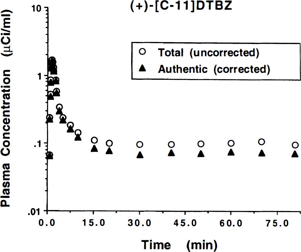
Plasma radioactivity concentration time course for equilibrium studies. Plotted are the total (open circles) and authentic (solid triangles) (+)-α-[11C]DTBZ concentration in arterial plasma over the 80-minute study duration. The administration protocol consists of a partial loading bolus of 50% of the dose (9 mCi) delivered over the first minute of the study followed by continuous infusion of the remainder of the dose (9 mCi) over the remaining 79 minutes of the study. Values have been corrected for radioactive decay. Equilibrium in blood is reached by 20 to 30 minutes into the study.
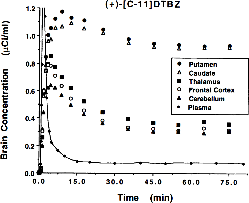
Brain radioactivity concentration time course for equilibrium studies. Plotted are the tissue time–activity curves for five brain regions over the 80 minutes' study duration. The administration is the same as described in Fig. 1. Values have been corrected for radioactive decay. Equilibrium is reached in all regions by 30 to 40 minutes into the study.
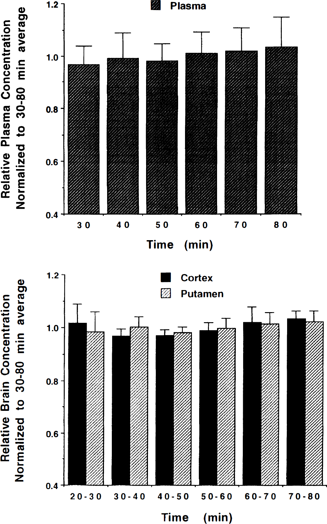
Stability of plasma and brain radioactivity concentration at equilibrium. Shown are the group mean and standard deviation of concentration values for both metabolite corrected arterial plasma (top) and brain regions with both high and low binding (bottom) during the equilibrium phase of the study. All data sets (plasma, cortex, putamen) for each of the nine subjects were normalized to the mean concentration measured over the 30- to 80-minute period. Thus, values over the entire time period averages 1 for not only the group but each individual subject.
A second objective was to verify that the change in input function shape for infusion studies compared with bolus injection studies did not cause differences in the kinetic estimates of VMAT2 binding. Figure 4 presents DVtot(kin) estimates using the pixel-by-pixel weighted integral analysis with 60 minutes of data for the current continuous infusion study (n = 9; solid bars) compared with those from our previous bolus injection study (n = 7; shaded bars). Shown are the mean and standard deviation of each group for the five regions analyzed. No statistically significant differences were detected in any of the five regions (P > 0.25). Similar results were obtained for the other kinetic methods, which also yielded no statistically significant differences between bolus and continuous infusion studies.
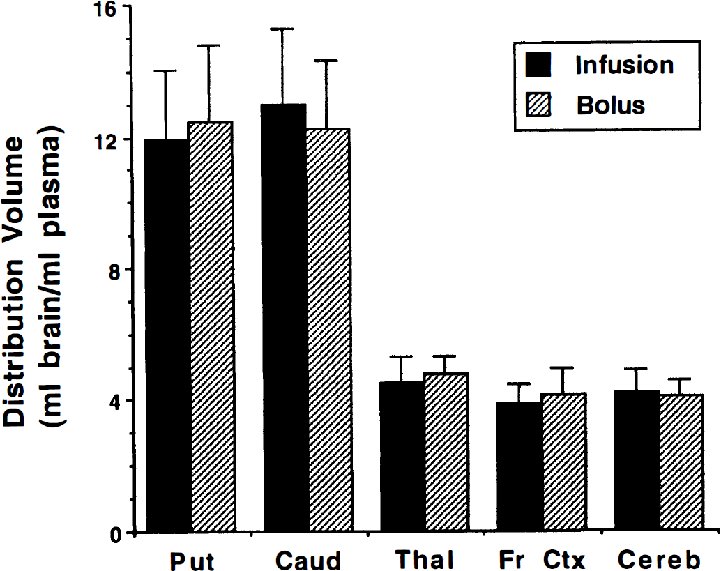
Comparison of binding estimates from bolus-plus-infusion and bolus (+)-α-[11C]DTBZ studies. Kinetic estimates of DVtot using weighted integral analysis from continuous infusion studies (solid bars) are compared with those from previous bolus injection studies (shaded bars). Shown are group means and standard deviations for the two groups (bolus plus continuous infusion, n = 9; bolus injection, n = 7). No significant differences were detected between DVtot estimates obtained using the two administration protocols.
Our third and primary objective in this study was to compare estimates of VMAT2 binding from equilibrium analysis with those from kinetic analyses of the same data sets. Table 1 reports group mean and standard deviations of DVtot for each of the methods using data to 60 minutes. Coefficients of variation were approximately 20% and found to be nearly identical both across methods and across regions. Also given are the group mean and across subjects standard deviation of the percent difference between each of the kinetic methods and the equilibrium method. A two-factor repeated measures analysis of variance was performed with method and region as repeated measures. The analysis included a method by region interaction term. Since the across subjects standard deviations were not equivalent for the different regions but proportional to the regional means (i.e., equal regional coefficients of variation), a logarithmic transformation of DVtot was used to stabilize the variances. Results indicate that there were significant differences across analysis methods (P < 0.0001) as well as the known differences across regions (P < 0.0001). In addition, a significant region by method interaction (P = 0.0015) was detected. Subsequent two-tailed paired t tests were performed, testing directly for differences between DVtot(eq) and each measure of DVtot(kin). The P values for these test are reported in Table 1.
Comparison of kinetic and equilibrium estimation of DVtot for (+)-(α)-[11C]DTBZ
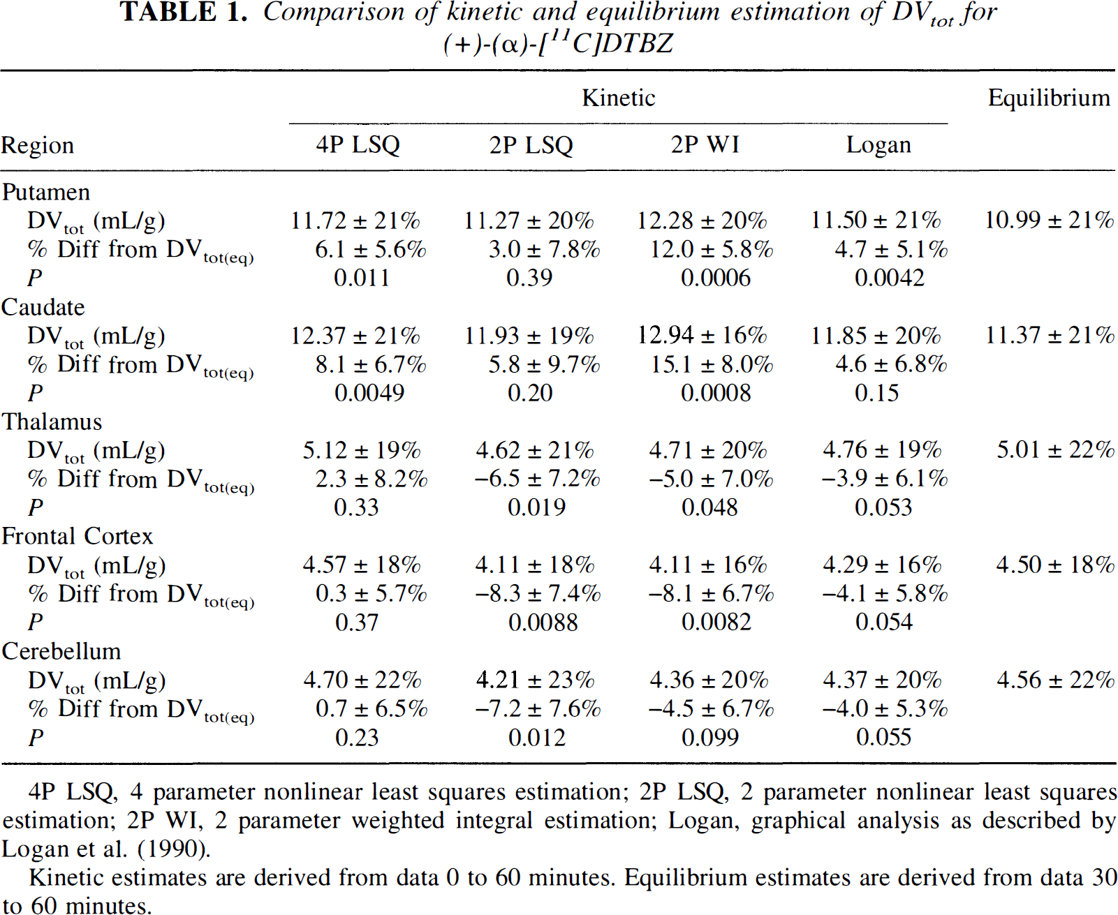
4P LSQ, 4 parameter nonlinear least squares estimation; 2P LSQ, 2 parameter nonlinear least squares estimation; 2P WI, 2 parameter weighted integral estimation; Logan, graphical analysis as described by Logan et al. (1990).
Kinetic estimates are derived from data 0 to 60 minutes. Equilibrium estimates are derived from data 30 to 60 minutes.
The uniformity of the coefficients of variation across analysis methods indicates there is not likely to be major differences in precision of DVtot between the methods; however, intersubject variability, if high, may mask smaller intermethod differences in precision. Since the true values for DVtot are not known, the precision of the methods is not readily determined. One indicator of precision is to look at the functional images created from pixel-by-pixel estimations of DVtot for the various methods. Figure 5 shows pixel-by-pixel DVtot images at three different brain levels created by the weighted integral, Logan plot, and equilibrium methods. The left two columns show weighted integral and Logan plot DVtot estimations from one of the seven bolus injection studies included in the data presented in Fig. 4. The right three columns show weighted integral, Logan plot, and equilibrium DVtot estimations for a typical bolus-plus-infusion scan from the current study. The top row of images are shown at a level through the caudate nucleus and putamen and are windowed to show the full dynamic range of DVtot in DTBZ studies. The following rows show three brain levels windowed down by a factor of 3.0 to highlight areas of low binding. Row 3 shows the same brain levels as row 1, whereas rows 2 and 4 show slices approximately 3.5 cm higher and 3.5 cm lower, respectively, than those in row 3. Effects of differing administration protocols (bolus versus bolus-plus-infusion) can be seen by examining columns 1 and 2 compared with columns 3 and 4. Effects of kinetic versus equilibrium analysis methods applied to the same set of data can be examined by comparing columns 3 through 5.
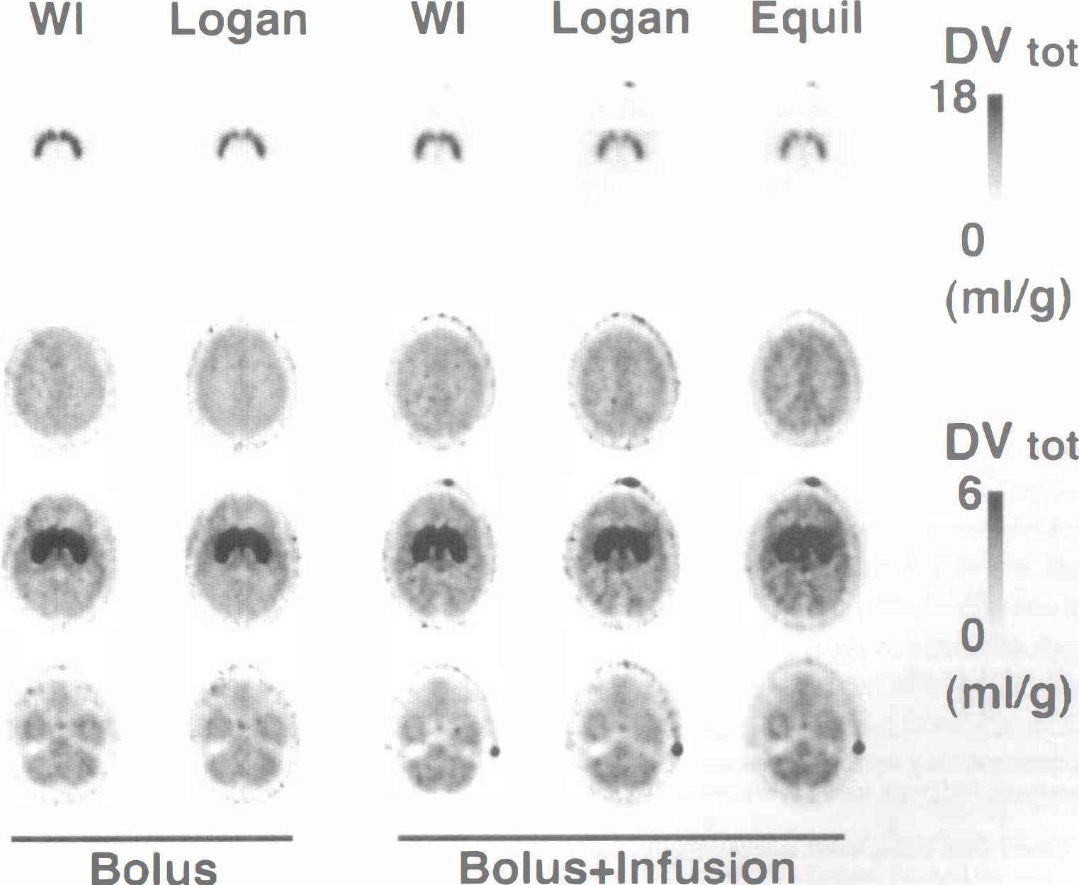
Parametric DVtot images. Displayed are pixel-by-pixel DVtot images at three different brain levels created by the weighted integral (WI), Logan plot (Logan), and equilibrium (Equil) methods. The left two columns show functional images of DVtot from a bolus injection study. The right three columns show functional images of DVtot from a bolus-plus-infusion study. The top row of images are at a level through the caudate nucleus and putamen, and show the full dynamic range of the studies (peak DVtot = 18 mL/g). The following rows show three brain levels windowed down by a factor of 3.0 to highlight areas of low binding (peak DVtot = mL/g). Row 3 shows the same brain levels as row 1, whereas row 2 slices are about 3.5 cm higher and row 4 slices are about 3.5 cm lower than those in row 3.
Two independent observers rated the statistical quality of DVtot image sets for each of the seven bolus injection subjects and each of the nine bolus-plus-infusion subjects. Both observers rated the DVtot images from the bolus studies to be slightly superior on average to those from the bolus-plus-infusion subjects for both weighted integral and Logan plot methods. There was considerable overlap, but the three highest rated images sets were from bolus studies, whereas the four lowest rate sets were from bolus-plus-infusion studies. Differences in statistical quality between the weighted integral, Logan plot, and equilibrium methods within the bolus-plus-infusion group were judged to be minimal, with no consistent preference for any one method.
The region by method interaction mentioned above can be appreciated better by examining the ratio between high and low binding regions, as seen in Table 2, where group means and standard deviations are reported for DVtot normalized to frontal cortex. Coefficients of variation for the normalized binding estimates were considerably smaller than those for the absolute estimates, the usual finding in most PET studies. Also given are means and standard deviations for the percent differences in DVtot(kin) relative to DVtot(eq) and the P values for paired t tests comparing kinetic and equilibrium methods. The kinetic methods exhibit higher contrast between high and low binding regions than the equilibrium method. This was especially moticeable for the weighted integral method, where the normalized DV values in caudate and putamen were more than 20% greater than the equilibrium method. Figure 6 gives the group means and across subjects standard deviations of the ratio DVtot(kin)/DVtot(eq) or the four-parameter least-squares and pixel-by-pixel Logan plot measures relative to the equilibrium measure. The larger DVtot ratios in the higher binding density regions (putamen and caudate nucleus) than in the lower density regions (thalamus, cortex, and cerebellum) indicates the greater contrast of the kinetic methods.
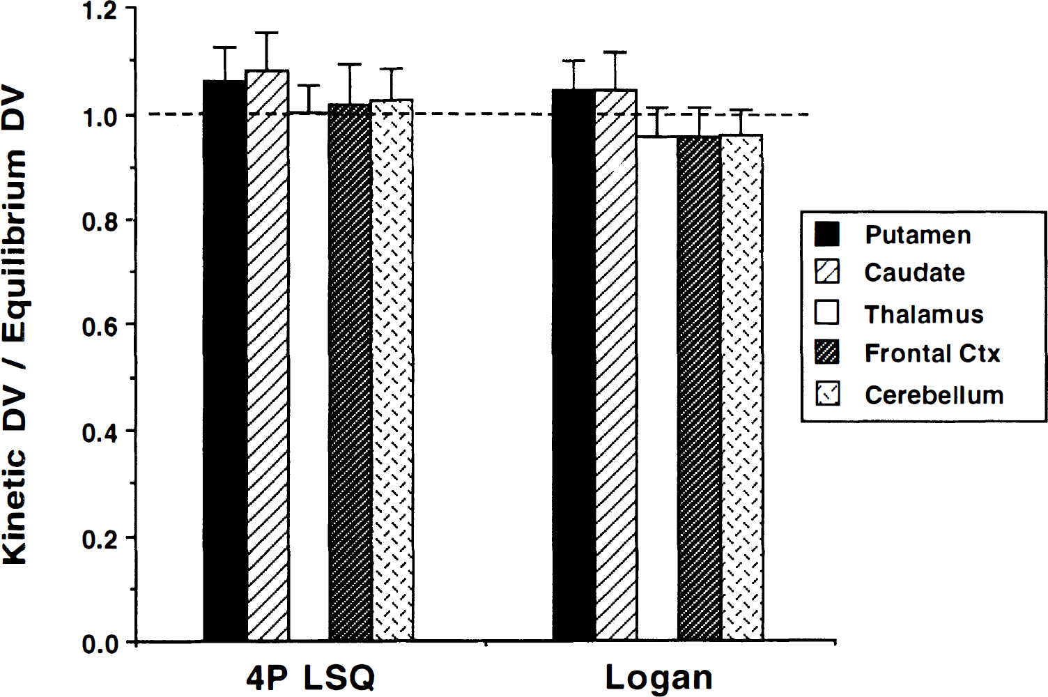
Ratio of kinetic to equilibrium estimates of (+)-α-[11C]DTBZ DVtot. Comparisons of both a four-parameter nonlinear least-squares analysis (4P LSQ) and pixel-by-pixel Logan plot analysis with the equilibrium approach are presented for the five brain regions. Values are group mean and standard deviation of the ratio DVtot(kin)/DVtot(eq).
Comparison of kinetic and equilibrium estimation of DVtot frontal cortex
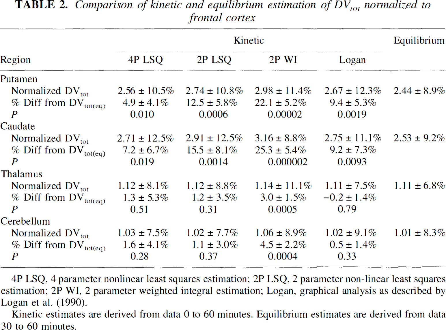
4P LSQ, 4 parameter nonlinear least squares estimation; 2P LSQ, 2 parameter non-linear least squares estimation; 2P WI, 2 parameter weighted integral estimation; Logan, graphical analysis as described by Logan et al. (1990).
Kinetic estimates are derived from data 0 to 60 minutes. Equilibrium estimates are derived from data 30 to 60 minutes.
Although we found only relatively small differences between kinetic and equilibrium methods, we were interested in examining the correspondence of the approaches across individual subjects as well as across different brain regions. Table 3 shows results from linear regression analysis between the different methods. Correlation coefficients based on DVtot estimates from 45 volumes-of-interest (5 brain regions from 9 subjects) and the mean absolute difference between the two methods for the same 45 values are reported to the lower left of the diagonal. Correlations between the various kinetic methods are all high (over 0.99). Correlations between the equilibrium method and each of the kinetic methods (bottom row) are not as strong, but still range from 0.977 and 0.989. The weighted integral method appears to be the most different from other methods based on the mean absolute differences between it and the other methods. Regression slopes and intercepts (in parentheses) are reported to the upper right of the diagonal. For each regression, the parameter in the row heading corresponds to the ordinate, whereas the parameter from the column heading corresponds to the abscissa. Thus, regressions of each of the kinetic methods on the equilibrium method are given in the right-most column. The higher contrasts of the kinetic methods described earlier appear as regression slopes greater than unity. The regression between the three-compartment four-parameter kinetic method and the equilibrium method is illustrated in Fig. 7.
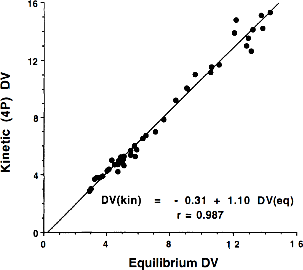
Relation between DVtot(kin) and DVtot(eq). The kinetic estimation (ordinate) is obtained using the four-parameter least-squares method. The plot contains data from five regions for each of the nine subjects.
Regression analysis of binding measures between methods
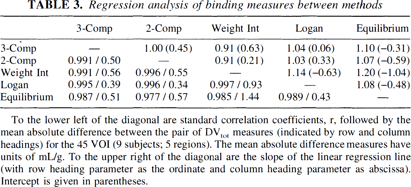
To the lower left of the diagonal are standard correlation coefficients, r, followed by the mean absolute difference between the pair of DVtot measures (indicated by row and column headings) for the 45 VOI (9 subjects; 5 regions). The mean absolute difference measures have units of mL/g. To the upper right of the diagonal are the slope of the linear regression line (with row heading parameter as the ordinate and column heading parameter as abscissa). Intercept is given in parentheses.
The effects of study duration on DVtot estimates for both kinetic (four-parameter least-squares) and equilibrium methods are presented in Fig. 8. Neither method depends strongly on duration. The kinetic estimates are slightly lower when using only 60 minutes of data (averaging 1% to 5%, depending on the region), whereas equilibrium estimates (group average) differ by less than 0.5% for all regions. The variability between the 60- and 80-minute DVtot estimates across individual subjects is low, but slightly higher for the equilibrium method (4% to 5%) than for the kinetic methods (3% to 4%).
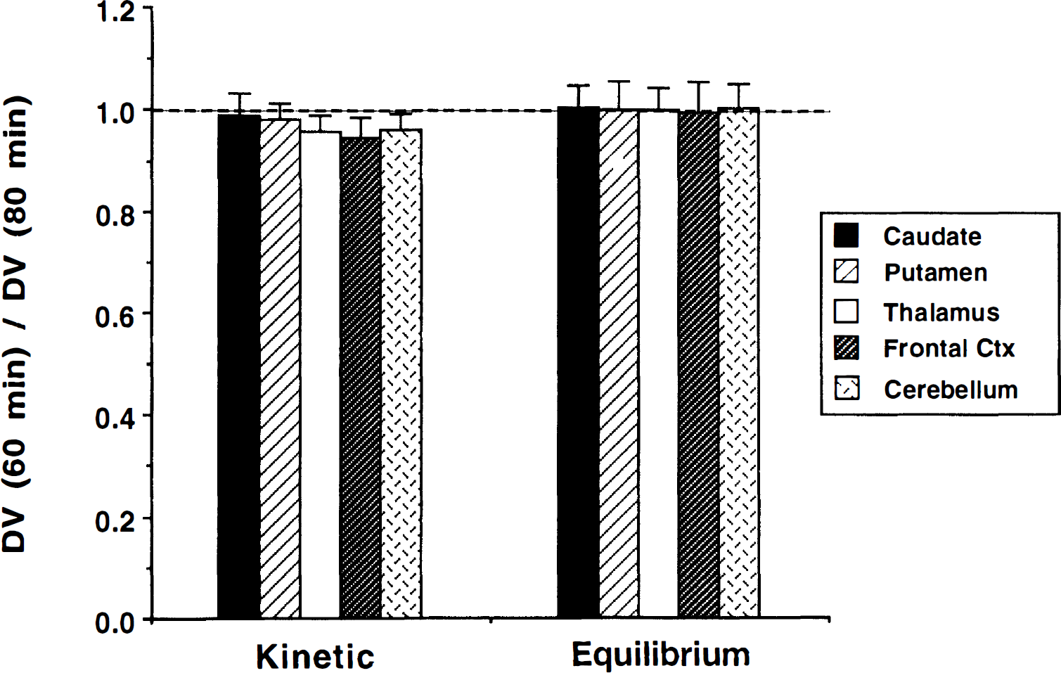
Ratio of DVtot derived from scan durations of 60 and 80 minutes of data for kinetic and equilibrium analyses. Kinetic DVtot is obtained using the four-parameter least-squares method. Data from 0 to 60 and 0 to 80 minutes were used for kinetic estimates, whereas data from 30 to 60 and 30 to 80 minutes were used for equilibrium estimates.
DISCUSSION
In previous work, we have demonstrated that the estimation of the total tissue distribution volume, DVtot, yields a precise and reliable measure of the density of binding sites for the vesicular monoamine transporter (Koeppe et al., 1996). Whereas the procedure is relatively simple, requiring only a single tracer injection and 60 to 80 minutes of scanning, we were interested in testing a protocol that would be even simpler to perform and more easily tolerated by patients who may otherwise be difficult to study. Since the equilibrium ratio of total concentration of tracer in tissue to the concentration of authentic tracer in arterial plasma is the definition of DVtot, an equilibrium protocol such as has been used by many groups in the PET field for a variety of reversible tracers is well suited for assessing the level of (+)-α-[11C]DTBZ binding to the vesicular monoamine transporter. In this work, we compare results using an equilibrium administration and analysis protocol to least-squares and pixel-by-pixel kinetic approaches for estimating DVtot
The primary assumption required for the equilibrium method is that blood and tissue reach equilibrium before the initiation of scanning. If true equilibrium is not fully reached, the tissue–to–arterial plasma concentration ratio may not accurately reflect the true values of DVtot. The rates of ligand–transporter association and dissociation relative to the rate of change of the plasma concentration determine the degree of error in the DVtot estimate, as discussed by Carson and colleagues (1989). To more rapidly achieve equilibrium conditions between plasma and the tissue compartments, we used a tracer administration protocol consisting of a partial loading bolus followed by continuous infusion of tracer. The relative fraction of the total dose to be administered in the initial bolus depends on the clearance rate of the slowest component from tissue or blood, as described previously (Frey et al., 1985, Carson et al., 1989). If continuous infusion alone is used or if too small a fraction is given as the loading bolus, equilibrium is delayed, since the blood and tissue concentrations must continue to climb to reach equilibrium. However, if too great a fraction is given initially, clearance of tracer must occur before reaching equilibrium. Based on the plasma clearance in the seven subjects of the initial kinetic studies reported in (Koeppe et al., 1996), we selected a 50:50 split between bolus and continuous administration fractions for the 80-minute study. The average plasma clearance 30 minutes after bolus injection for these seven subjects was 0.013 min−1. Considering that a unit dose (1.0) is given as the initial bolus and that there is approximately 1.3% clearance per minute, 1.3% of the bolus dose per minute needs to be replaced. Thus, for a 1-minute “bolus” injection followed by 79 minutes of continuous infusion, a total of 0.013 × 79 units of dose, or 1.03 times the dose given as a bolus, is needed to achieve equilibrium in plasma. Thus, nearly a 1:1 ratio between bolus and infusion portions of the total dose will rapidly reach equilibrium in blood. These are decay-corrected fractions, not absolute doses, since we decay-corrected both arterial plasma and PET data.
The first three figures demonstrate our ability to achieve near equilibrium conditions by approximately 30 minutes after the loading bolus. For the particular subject shown in Figs. 1 and 2, there was a small net clearance in all regions after the initial loading bolus, and, therefore, equilibrium would have been reached more quickly with a slightly smaller bolus fraction. However, for other subjects, the higher binding regions of caudate and putamen demonstrated no net clearance but continued to increase for some time after the initial bolus, indicating that a slightly higher initial bolus fraction would have been better. Whereas a higher bolus fraction would delay equilibration in the lower binding regions, it is the higher binding regions that are more susceptible to errors caused by nonequilibrium conditions (Carson et al., 1989), and thus these are the regions that require greater attention. On the average, a 50:50 split for an 80-minute study appears to be nearly optimal. For our nine subjects, six showed trends toward increasing concentrations, whereas three showed decreases, indicating that the optimal split varies from subject to subject (depending on individual plasma clearance rates and rate parameters for brain transport and binding). For shorter studies (e.g., 60 minutes), the fraction given as a bolus would need to be increased (since the last 20 minutes of the study is omitted). In this case, closer to 60% of the total should be given as the loading bolus.
Data presented in Figs. 4 and 5 demonstrate that the change in input function shape for this experiment did not have a major effect on the estimates of DVtot(kin) in any of the brain regions under examination. Results shown in Fig. 4 were obtained from pixel-by-pixel weighted integral analysis and showed no significant differences between bolus and bolus-plus-infusion groups. Comparisons with the nonlinear least-squares and Logan plot analyses gave similar results, also yielding no statistically significant differences. On average, the statistical quality of the parameter images of DVtot were slightly better for the bolus injection studies than for the bolus-plus-infusion studies. This may be due in part to the shape of the input curve producing a tissue curve with less distinct temporal changes. However, this also may result from the fact that bolus subjects received a full 18-mCi injection, whereas the bolus-plus-infusion subjects received 9 mCi as a bolus followed by 9 mCi (in the syringe at time of injection) administered over the next 79 minutes. Because of decay in the syringe, only slightly greater than 3 of the final 9 mCi, or a total of 12 mCi, actually is administered to the subject. Overall, these results demonstrate that the kinetic estimates of VMAT2 binding density derived using the equilibrium acquisition protocol are consistent with kinetic estimates derived from our previous bolus injection protocol and, therefore, the kinetic estimates from the current study serve as a valid comparison for the equilibrium estimates derived from these same data sets.
The results presented in Table 1 and Fig. 5 show the distribution volume estimates from the equilibrium method to be consistent with those from the kinetic methods. The coefficients of variation of the equilibrium estimates reported in Table 1 were nearly identical to those of the kinetic estimates, and, like the kinetic methods, exhibited almost no regional variability. The functional images in the right-most three columns of Fig. 5 demonstrate the degree of correspondence between the pixel-by-pixel kinetic and the equilibrium methods. Independent observers viewing images sets from all nine subjects rated the statistical quality of each of the three methods as being nearly identical.
The most consistent difference among the methods was the contrast between high and low binding regions. This can be seen in the results presented in several of the tables and figures, including the subject shown in the right-most three columns of Fig. 5. The weighted integral approach yields higher DVtot values in the basal ganglia than either the Logan or equilibrium methods (row 1, columns 3 to 5) while yielding the lowest DVtot values in the cortex, thalamus, and cerebellum (rows 2 to 4), with equilibrium images yielding the highest values. Table 2 gives binding values normalized to frontal cortex, whereas Fig. 6 shows ratios of kinetic to equilibrium DVtot estimates. Normalized DVtot in high-binding regions of caudate nucleus and putamen are lower for the equilibrium method than for any of the kinetic methods. However, contrast between high and low binding regions varies among the kinetic measures as well. The weighted integral and two-parameter least-squares kinetic methods, both based on a single-tissue model configuration, have higher contrast than the four-parameter least-squares and Logan plot analyses, which are based on multicompartment configurations. The higher contrast is likely caused by the inability of a two-compartment configuration to describe (+)-α-[11C]DTBZ kinetics, particularly for regions of low binding density. Examination of the residuals from the four-parameter fits does not reveal a pattern that would cause overestimation in DVtot(kin) in regions of high binding density. The observed pattern of residuals, however, is consistent with slight underestimations in DVtot(kin), particularly in regions of low binding density. This may contribute in part to the observed increase in contrast between basal ganglia and cortex in the kinetic methods.
Another factor that may explain lower DVtot values as well as lower contrast in the equilibrium method compared with the kinetic methods is that the vascular activity was ignored in the calculation of DVtot(eq). The concentration measured by PET is given by (1-CBV)Ct + CBV Cbl, where CBV is the vascular fraction in brain and Ct and Cbl are the tissue and total blood concentrations, respectively. Thus, the measured DVtot, without correction for vascular activity, is given by DVtot = [(1 − CBV)Ct + CBV Cbl]/Cp, where Cp is the authentic plasma concentration. The ratio Cbl/Cp approximately equals 2.0, since the red cell and plasma concentrations are nearly the same and there are about 50% metabolites. Thus, the measured DVtot is approximated by (1 − CBV) DVactual + 2 CBV, where DVactual is the correct DVtot value. For a vascular fraction of 4% and DVactual of 12 mL/g (typical for basal ganglia), the measured DVtot would equal 11.6 mL/g, an underestimation of 3.3%. For a DVactual of 4.0 mL/g (typical for cortex), the measured DVtot would equal 3.92 mL/g, an underestimation of only 2%. This partly explains the lower DVtot values observed in basal ganglia and a contrast reduction of around 1.5%, but not the 5% to 7% or more reduction actually observed.
Examination of the degree to which equilibrium is achieved, as assessed by any net increase or decrease in the tissue concentration after 30 minutes, does not support a decrease in contrast between high and low binding regions for equilibrium analysis. Since the tissue responds to fluctuations in the plasma concentration and not the reverse, changes in the tissue concentration lag behind changes in the plasma. This lag is greater in regions of higher binding where tissue and blood equilibrate more slowly. A decline in plasma concentration causes overestimates in DVtot that are greater in higher binding regions, therefore causing contrast enhancement, whereas a slow rise in plasma concentration would cause the opposite. Since six of nine subjects had increases and only three of nine had gradual decreases in plasma concentration over time, we thought that we might find a difference in contrast between the two subgroups. However, when the subjects were separated in this manner, no differences in contrast were seen in DVtot(kin)/DVtot(eq) between basal ganglia and cortex: all nine subjects showed contrast reduction in the equilibrium analysis compared with the kinetic analyses.
Whereas the previous discussion focused on consistent biases in DVtot estimates between the methods (differences in group means), we also were interested in how well equilibrium measures correlated with kinetic measures subject-by-subject as well as region-by-region. The results presented in Table 3 (lower left of diagonal) demonstrate high correlations between equilibrium and kinetic measures (range 0.977 to 0.989). The three-compartment four-parameter and the Logan plot estimations had higher correlations and also the smaller mean absolute differences relative to the equilibrium method than did the other kinetic methods, suggesting errors occur when using a two-compartment configuration, which is not fully able to describe the kinetic behavior the tracer. Correlations among the various kinetic measures were slightly higher, as might be expected, ranging from 0.991 to 0.997. A plot of the four-parameter DVtot(kin) versus DVtot(eq) estimates across the nine subjects and five regions (Fig. 7) suggests that there is greatest variability between the methods in the regions with the highest VMAT2 densities. Comparisons of the other DVtot(kin) measures with DVtot(eq) show similar patterns, again with the greatest discrepancy being in the regions of highest binding. This increased variability in the high binding regions is less noticeable in plots between the various kinetic measures, and thus the slightly lower correlation between the equilibrium and the kinetic DVtot estimates are due almost entirely to these few highest values.
The duration of data used was found to have little effect on the estimates of DVtot, as seen in Fig. 8. This was particularly true for equilibrium estimates. We did detect small, relatively consistent differences in the kinetic methods where 60-minute DVtot(kin) estimates were slightly lower than estimates using 80 minutes of data. These differences were greater for regions of low binding than regions of high binding. Examination of the residuals to the kinetic fits, even when using a three-compartment model configuration, typically reveals that the predicted tissue curve is slightly lower at 50 to 60 minutes than the measured data points. With the inclusion of the additional 20 minutes of data, the fitted curve appears to be more consistent with the measured data. This results in the DVtot(kin) estimates being slightly lower when only 60 compared with 80 minutes of data are used in the fit. This pattern is more noticeable in low binding regions, and therefore the effects shown in Fig. 8 are more noticeable for the thalamus, frontal cortex, and cerebellum than for the basal ganglia. The equilibrium estimates show no differences between analyses using 30 to 60 or 30 to 80 minutes of data, with group mean differences being less than 0.5% in all regions. This result confirms that we have achieved equilibrium sufficiently such that data from 30 minutes and later can be used to estimate DVtot(eq). Variability of the 60/80 minutes DVtot(eq) ratio across individual subjects is slightly higher than for the DVtot(kin) ratio. This may likely result from the fact that only a portion of the data is used in the equilibrium calculation, compared with the entire data sequence being used for kinetic estimations, and thus statistical noise or any potential biases (such as patient motion) in individual scans, may have a greater impact on the estimate of DVtot(eq) than on DVtot(kin).
Since we were interested in comparing results between kinetic and equilibrium methods, our acquisition protocol included multiple samples for both arterial plasma and brain (PET). In theory, only a single scan and single blood sample is required for calculation of DVtot, once equilibrium is achieved. However, for practical reasons, we propose that even a streamlined acquisition protocol should include multiple PET scans that are no more than 10 minutes long and blood samples approximately every 10 minutes. This protects against losing a study because of severe patient motion part way through the scan or a bad blood sample. In our standard protocol, for determining DVtot, we now acquire three 10-minute scans from 30 to 60 minutes after the beginning of tracer administration, while acquiring blood samples at 30, 40, 50, and 60 minutes.
Overall, we detected only relatively minor differences between the methods, with the equilibrium values being lowest in high binding regions. However, since no gold standard measure exists with which to compare results from any of these methods, it is difficult to assess which is most accurate. The precision was similar for all methods, and therefore, the choice of the most favorable method depends primarily on the specific biases associated with each approach. It might be predicted that the kinetic approaches would show the greatest similarity, since they all depend on data throughout the entire study, not just during the equilibrium phase. This was what we saw as indicated by the higher correlations between any combination of kinetic methods (r ≥ 0.991) than between the equilibrium method and any one of the kinetic methods (r ≤ 0.989). One might also expect that the two-parameter least-squares and weighted integral kinetic approaches show a high degree of similarity, since they both require rapid equilibration between free and bound compartments, whereas the four-parameter least-squares, the Logan, and the equilibrium approaches do not require this assumption. This was not observed, but instead the weighted integral method was found to exhibit the greatest difference from the other methods in regions of high binding, which may result from the inherent difference in how biases caused by failure of the rapid equilibration assumption propagate into the DVtot estimate for this method. Both the regression slopes (upper right of diagonal) and the mean absolute differences between methods (lower left of diagonal) reported in Fig. 7 also suggest that the weighted integral method performs unlike the others. In comparisons involving the weighted integral method, the regression slopes are most different from unity and the mean absolute differences are the largest. Of the four kinetic approaches, the Logan method exhibits the highest correlations with and the smallest mean absolute differences relative to the equilibrium method. Taking all of these results into account, and because of the fewer overall assumptions and inherent greater simplicity of the approaches, we believe that the Logan calculation and the equilibrium method provide the most accurate measures of DVtot, although the difference in performance from the other approaches is small. Other factors, such as whether an accurate estimate of K1 is required, still may influence the final selection of which method to adopt.
In summary, we have shown that an equilibrium approach to (+)-α-[11C]DTBZ imaging is easily performed and the data easily analyzed. Although the experimental protocol in this study involved acquisition of a full dynamic sequence of PET scans and numerous blood samples to allow kinetic analysis, a procedure streamlined for equilibrium analysis requires only a single scanning interval of 30 minutes or less and a few blood samples. An administration protocol consisting of a loading bolus followed by continuous infusion can provide steady-state conditions in both blood and tissue by approximately 30 minutes. We have demonstrated a high degree of correspondence between kinetic and equilibrium estimates of the total (+)-α-[11C]DTBZ distribution volume. The coefficients of variation of the kinetic and equilibrium DVtot estimates were nearly identical in all regions examined, both for absolute and for normalized measures. The statistical quality of data and hence the precision of the methods also appear to be similar. Correlations between kinetic and equilibrium estimates across both subjects and regions exceeded 0.975. A slightly lower contrast (7% to 10%) between regions of high and low VMAT2 binding density was observed for the equilibrium method compared with the kinetic methods; however, this difference was consistent across subjects. We conclude that a simple protocol using a loading bolus followed by continuous infusion of (+)-α-[11C]DTBZ can provide excellent measures of VMAT2 binding.