Sage Journals: Discover world-class research

Abstract

(+)-α-[¹¹C]Dihydrotetrabenazine (DTBZ) binds to the vesicular monoamine transporter (VMAT2) located in presynaptic vesicles. The purpose of this work was to evaluate various model configurations for analysis of [¹¹C]DTBZ with the aim of providing the optimal measure of monoamine vesicular transporter density obtainable from a single dynamic PET study. PET studies on seven young normal volunteer subjects, ages 20–35, were performed following i.v. injection of 666 ± 37 MBq (18 ± 1 mCi) of (+)-α-[¹¹C]DTBZ. Dynamic acquisition consisted of a 15-frame sequence over 1 h. Analysis methods included both creation of pixel-by-pixel functional images of transport (K₁) and binding (DV_tot) and nonlinear least-squares analysis of volume-of-interest data. Pixel-by-pixel calculations were performed for both two-compartment weighted integral calculations and slope-intercept estimations from Logan plots. Nonlinear least-squares analysis was performed applying model configurations with both two-compartments, estimating K₁ and DV_tot, and three compartments, estimating K₁-k₄. For the more complex configuration, we examined the stability of various binding-related parameters including k₃ (k_onB_max′), k₃/k₄ (B_max′/K_d), DV_sp [(K₁/k₂)(k₃/k₄)], and DV_tot [K₁/k₂(1 + k₃/k₄)]. The three-compartment model provided significantly improved goodness-of-fit compared to the two-compartment model, yet did not increase the uncertainty in the estimate of the DV_tot. Without constraining parameters in the three-compartment model fits, DV_tot was found to provide a more stable estimate of binding density than either k₃, k₃/k₄, or DV_sp. The two-compartment least-squares analysis yielded approximately 10% underestimations of the total distribution. However, this bias was found to be very consistent from region to region as well as across subjects as indicated by the correlation between two- and three-compartment DV_tot estimates of 0.997. We conclude that (+)-α-[¹¹C]DTBZ and PET can provide excellent measures of VMAT2 density in the human brain.

Keywords

Tracer kinetics VMAT2 Monoamine vesicular transporter Positron emission tomography

The assessment of cerebral biochemistry in living persons via the use of radiolabeled tracers and positron emission tomography (PET) has been a widely explored field over the past decade. The purpose of this study is to characterize the in vivo kinetic behavior of (+)-α-[¹¹C]dihydrotetrabenazine (DTBZ) binding to the vesicular monoamine transporter (VMAT2). The VMAT2 binding site is a specific protein located exclusively in the membranes of presynaptic vesicles (Henry and Scherman, 1989) and radioligands for VMAT2 have been proposed as both in vitro (Scherman et al., 1988; Near, 1986; Masuo et al., 1990) and noninvasive in vivo (DaSilva and Kilbourn, 1992) markers of nigrostriatal neurons. Prior studies in our laboratories have demonstrated a regional in vivo brain binding of such radioligands, which correlate with the known distribution of VMAT2 in rodent brain (Kilbourne, 1994; Kilbourn et al., 1995), and the linear relationship between the level of in vitro striatal radioligand binding to VMAT2 and the extent of nigral injury in 6-hydroxydopamine-lesioned rats (Vander Borght et al., 1995). DTBZ exhibits high affinity (low nanomolar) binding only to VMAT2, while animal studies have shown a lack of regulation of this transporter by repeated or chronic dopaminergic or cholinergic drug treatments (Naudon et al., 1994; Vander Borght et al., 1995; Wilson and Kish, 1996). This is in contrast to other aspects of the dopaminergic nerve terminal, including dopamine synthesis and the neuronal membrane dopamine transporter, where drug-induced regulation of the enzyme (Zhu et al., 1992; Hadjiconstantinou et al., 1993; Gjedde et al., 1993) or transporter (Ikegami and Prasad, 1990; Kilbourn et al., 1992; Sharpe et al., 1991; Wiener et al., 1989; Wilson et al., 1994) has been clearly demonstrated. While DTBZ binding is not specific to dopaminergic nerve terminals, as the radioligand binds to the vesicular transporter common for all monoaminergic neurons, the PET signal measured in the striatum largely represents storage vesicles in the predominant (>95%) dopaminergic terminals (Kish et al., 1992). DTBZ binding to the VMAT2 is thus complimentary to but distinctly different from previous PET and SPECT radiotracers that have been proposed for the study of nigrostriatal pathology, including those that follow dopamine synthesis and storage, such as [¹⁸F]fluorodopa (Garnett et al., 1983; Gjedde et al., 1991; Huang et al., 1991) and [¹⁸F]fluoro-m-tyrosine (DeJesus et al., 1995), or those that bind to the neuronal membrane dopamine transporter, such as [¹¹C]nomifensine (Aquilonius et al., 1987, Salmon et al., 1990), [¹¹C]WIN 35,428 (Frost et al., 1993), [¹⁸F]GBR 12909 (Koeppe et al., 1990), and [¹²³I] ß-CIT (Innis et al., 1993; Laruelle et al., 1994).

In this work, we present an evaluation of kinetic analysis approaches for the estimation of a VMAT2 density index following a single radioligand injection. Each approach provides separate estimates for parameters representing the tracer's blood-brain barrier (BBB) transport rate and tissue distribution volume. We examined both pixel-by-pixel estimation procedures capable of producing functional images of the transport and binding parameters and volume-of-interest (VOI) approaches using two- and three-compartment model configurations estimating two, three, or four rate parameters as well as accounting for the contribution of bloodborne radioactivity in the total PET signal. We compared the means and coefficients of variation (COV = SD/mean) to determine the appropriate trade-off between bias and precision in the parameter estimates. Computer simulation studies were performed in conjunction with the human studies to examine the magnitude of bias in the parameter estimates caused by various model simplifications or assumptions.

THEORY

Conceptually, the kinetic analysis of [¹¹C]DTBZ time-activity distribution begins with a model consisting of one blood compartment representing free ligand in arterial plasma (C_p) and three tissue compartments representing free ligand in tissue (C_f), nonspecifically bound ligand (C_ns), and specifically bound ligand (C_s). The first simplifying assumption that has been made throughout this work is that the free and nonspecific binding equilibrate rapidly and have been combined into a single compartment (C_f+ns). This three-compartment configuration has rate parameters defined as follows:

\begin{aligned} K_{1} & = f (1 - e^{- P S / f}) = f E_{0} ({m l g}^{- 1} min^{- 1}) \\ k_{2}^{'} & = K_{1} / (D V_{f + n s}) = (K_{1} / D V_{f}) / (1 + D V_{n s} / D V_{f}) (min^{- 1}) \\ k_{3}^{'} & = k_{o n} B_{max}^{'} / (1 + D V_{n s} / D V_{f}) (min^{- 1}) \\ k_{4} & = k_{o f f} (min^{- 1}) \end{aligned}

(1)

and thus,

k_{3}^{'} / k_{4} = (B_{max}^{'} / K_{d}) / (1 + D V_{n s} / D V_{f})

where f is mass specific blood flow (ml g⁻¹ min⁻¹), E₀ is the single pass extraction fraction of ligand across the BBB into brain, PS is the permeability surface area product (ml g⁻¹ min⁻¹), DV_f, DV_ns, DV_f+ns are the tissue distribution volumes of free ligand, nonspecifically bound ligand, and their sum, respectively (ml g⁻¹), k_on is the bimolecular association rate between ligand and receptor (g pmol⁻¹ min⁻¹), B_max′ is the binding site density or concentration of unoccupied transporter binding sites (pmol g⁻¹), k_off is the dissociation rate of ligand from the binding site complex (min⁻¹), and K_d is the equilibrium binding constant for the specific binding site (pmol g⁻¹ or nM). The “prime” symbols on k₂′ and k₃′ are used to differentiate these rate parameters from the true k₂ and k₃, which describe rates of exchange from the compartment containing only free ligand. The ratio of binding parameters B_max′/K_d has been previously referred to as the “binding potential” by Mintun et al. (1984). The term (1 + DV_ns/DV_f) reflects the apparent increase in volume of the binding precursor pool when combining free and nonspecific compartments. Thus, 1/(1 + DV_ns/DV_f) describes the fraction of radiolabel available either for transport back to plasma or binding to transporter sites and is equivalent to the term f₂ used by Mintun et al. (1984) and others. The distribution volumes of free + nonspecific, specific binding sites, and total are given by the following equations:

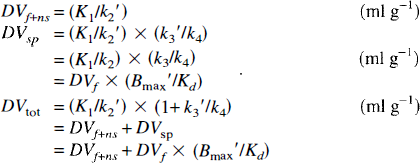
\begin{aligned} D V_{f + n s} & = (K_{1} / k_{2}^{'}) ({m l g}^{- 1}) \\ D V_{s p} & = (K_{1} / k_{2}^{'}) \times (K_{3}^{'} / k_{4}) \\ = (K_{1} / k_{2}) \times (K_{3} / k_{4}) ({m l g}^{- 1}) \\ = D V_{f} \times (M_{max}^{'} / k_{d}) \\ D V_{t o t} & = (K_{1} / k_{2}^{'}) \times (1 + K_{3}^{'} / k_{4}) ({m l g}^{- 1}) \\ = D V_{f + n s} + D V_{s p} \\ = D V_{f + n s} + D V_{f} \times (B_{max}^{'} / k_{d}) \end{aligned}

(2)

Because of the inherent difficulty in estimating individual rate parameters with high accuracy, particularly when the k₃ is large relative to k₂ (Koeppe, 1990; Koeppe et al., 1991; Frey et al., 1992) or when k₄ is small (Koeppe, 1990), and because of practical considerations necessitating that studies must be able to be implemented and performed routinely in human subjects, our group has intentionally pursued radioligands that exhibit both rapid binding and dissociation. The kinetic modeling of such ligands can often be simplified from the model described above to a model that combines all tissue compartments into a single compartment. This simplification is valid only when the binding and release of ligand from the specific binding sites is rapid compared to the transport parameters K₁ and k₂′. The meaning of the transport parameter K₁ is unchanged; however, the clearance parameter k₂ becomes:

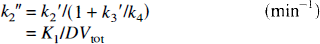
\begin{aligned} k_{2}^{''} & = k_{2}^{'} / (1 + k_{3}^{'} / k_{4}) (min^{- 1}) \\ = K_{1} / D V_{t o t} \end{aligned}

(3)

and thus,

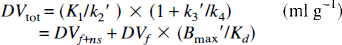
\begin{aligned} D V_{t o t} = (K_{1} / k_{2}^{'}) \times (1 + k_{3}^{'} / k_{4}) ({m l g}^{- 1}) \\ = D V_{f + n s} + D V_{f} \times (B_{max}^{'} / K_{d}) \end{aligned}

where DV_tot is the total distribution volume of the summed tissue compartments and has the same theoretical definition as DV_tot derived from the three-compartment approach. How closely the DV_tot estimates from the two different model configurations agree will depend primarily on how rapidly the free and bound compartments approach equilibrium (i.e., how valid the simplifying assumption is).

The primary goal of this study is to provide a reliable measure of vesicular monoamine transporter binding site density. In the ideal, this would be a direct quantitative measure of B_max′, the density of available binding sites; however, for practical reasons this may not be possible. As defined in Eqs. 1 –3, there exist other parameters that relate to binding density that might provide more reliable measures of binding density. These include $k_{3} (= k_{o n} B_{max}^{'}), k_{3} / k_{4} (= B_{max}^{'} / K_{d}), D V_{s p} [= D V_{f} \times (B_{max}^{'} / K_{d})], a n d D V_{t o t} [D V_{f + n s} + D V_{f} \times (B_{max}^{'} / K_{d})]$ . The distribution volume estimates, particularly DV_tot, are functions of more than just binding site density and therefore contain additional intrinsic bias compared to either k₃ or k₃/k₄. However, the precision of distribution volume estimates is typically much better than those of individual rate constants. It is the focus of this work to determine which measure yields the best trade-off between bias and precision and the greatest sensitivity to actual variations in binding site density.

MATERIALS AND METHODS

Seven young normal volunteers, 20–35 years of age, were studied following administration of 666 ± 37 MBq (18 ± 1 mCi) of (+)-α-[¹¹C]DTBZ. No-carrier-added [¹¹C]DTBZ (500–2,000 Ci/mmol) was prepared as reported by Kilbourn (1995). A sequence of 15 PET scans (4 × 30 s, 3 × 1 min, 2 × 2.5 min, 2 × 5 min, 4 × 10 min) was acquired on a Siemens/CTI ECAT EXACT-47 scanner (Knoxville, TN, U.S.A.) for 60 min following i.v. injection. Data were reconstructed using a Hanning filter with 0.5 (cycles/projection ray) cutoff. Calculated attenuation correction was performed on all images.

Blood samples were withdrawn via a radial artery catheter as rapidly as possible for the first 2 min of the scan and then at progressively longer intervals for the remainder of the study. Plasma was separated from red cells by centrifugation, and counted in a NaI well-counter. The plasma radioactivity time course was corrected for radiolabeled metabolites using a rapid Sep-Pak C₁₈ cartridge chromatographic technique similar to that previously reported for scopolamine and flumazenil (Frey et al., 1995). The samples at 1, 2, and 3 min and at all subsequent samples (13 in all) were analyzed for metabolites. Metabolite fractions of other samples prior to 2 min after injection were estimated by linear interpolation. Due to the relatively long scan duration, we employed a method using radioactive fiducial markers to correct for any patient motion occurring throughout the study. Molecular sieve beads (1–2 mm diameter) were placed at three points on the patient's scalp prior to the study. Approximately 1 μl of the ligand preparation was pipetted onto each bead at an activity of ˜2 μCi/bead. Following reconstruction of the dynamic PET sequence, the beads were defined on a single base frame (frame 10; 10–15 min after injection). Details of the reorientation method are described in Koeppe et al. (1991).

Volumes-of-interest (VOIs) were created on the base frame and applied to all other frames generating time-activity curves for the different brain structures. Regions analyzed included caudate nucleus, putamen, frontal cortex, thalamus, and cerebellar hemispheres. Left and right hemisphere regions were analyzed separately then averaged within each subject prior to calculation of group means and standard deviations. No significant hemispheric differences were detected.

Nonlinear least-squares analysis was performed on the VOI-generated time-activity data. Parameters were estimated for both two- and three-compartment configurations using the Marquardt algorithm (Bevington, 1969) with constraints restricting parameters (except time shift) to positive values. Each model configuration tested was implemented to account for the contribution from activity in the cerebral blood volume (CBV) and for the time offset or shift between the plasma input function measured from the radial artery and the actual arterial input to the brain. The time offset was estimated by fitting the entire slice average from a single mid-brain level to a three-compartment four-parameter model using the entire 60-min data set and assuming a whole-slice average CBV of 0.035 ml g⁻¹ (3.5%). In all subsequent fits for the subject, the time offset was fixed to this estimated value. Thus, each subject had a single value for the time offset (used for all regions) while CBV was estimated separately for each region. Even though rate constant estimates proved to be fairly insensitive to CBV and time shift, inclusion of both parameters in the model reduced the bias in K₁ caused by their effects on the early data. For the two-compartment configuration, K₁ DV_tot (K₁/k₂¶ime;), and CBV were estimated for each VOL For the three-compartment configuration, K₁, DV_f+ns (K₁/k₂′), k₃′, k₄, and CBV were estimated. Two other sets of fits were performed, both assuming a three-compartment configuration but with one parameter fixed to the mean value averaged across subjects. Estimates of K₁ DV_f+ns, k₃′, and CBV were obtained using the group mean value for k₄ for average across all regions (0.077 min⁻¹). Estimates of K₁ k₃′, k₄, and CBV were obtained using the group mean value averaged across all regions excluding basal ganglia for DV_f+ns (2.4 ml g⁻¹). Basal ganglia regions were excluded due to difficulties in differentiating free + nonspecific and specific compartments due to the higher rate of binding in these regions. The binding parameters k₃/k₄, DV_sp, and DV_tot were then calculated for each of these model configurations.

Two pixel-by-pixel analyses were also performed on the dynamic data sets. First, a two-parameter weighted integral analysis (Alpert et al., 1984) was implemented as previously used for [¹¹C]flumazenil (Koeppe et al., 1991) producing functional images of ligand delivery (K₁) and binding (DV_tot). The first 30 s of scan data was omitted from the calculations in order to reduce CBV effects on the estimated parameters. Second, a graphical analysis for reversible ligands was used to calculate DV_tot and an approximation for K₁. As discussed in their paper, the slope of the linear portion of the Logan plot yields an estimate of the total distribution volume of the ligand, DV_tot, independent of the number of compartments in the model. For ligand kinetics described by a two-compartment model, the plot is linear at all times, while for ligand kinetics requiring three (or more) compartments, linearity is not reached until some time later. The meaning of the intercept changes with model complexity and is easily interpretable only when a two-compartment model is assumed. The intercept is given by −1/[k₂¶ime;(1 + CBV/DV_tot)]. Ignoring blood volume contributions, this reduces to −1/k₂¶ime; and thus, K₁, can be approximated by the slope/-intercept. Pixel-by-pixel functional images of DV_tot were obtained from slope estimates using data beginning 10 min after injection, while images of K₁ were obtained from separate estimates of the slope and intercept made using the entire data set. Simulation and human studies were performed and the above time intervals were selected based on minimizing parameter bias caused by failure of the DTBZ kinetics to be described by a two-compartment model (see Discussion). After creation of K₁ and DV_tot images for both the weighted integral and Logan plot methods, the VOIs previously defined for kinetic analysis were applied to the functional images to obtain regional estimates of the model parameters.

RESULTS

The fraction of authentic [¹¹C]DTBZ in plasma decreased quite rapidly following administration, typically reaching 65–70% by 10 min, 50–60% by 30 min, then becoming relatively constant at 40–50% by 60 min after injection.

Results from least-squares fits to the DTBZ time-activity curves for two- and three-compartment model configurations are shown in Table 1. The entire 60-min data sequence was used in these fits. Table 1 values give the mean and percent coefficient of variation (COV; 100 × standard deviation/mean) of each parameter for the seven volunteers. The mean reduced chi-squared values (χ²; sum of the squared discrepancies between data and model predictions divided by the number of degrees of freedom) for fits to the regional time activity curves are reported for each model configuration.

Table 1.

Least-squares estimates of model parameters for two- and three-compartment model configurations

Region	2-compartment fits			3-compartment fits
Region	K₁ (ml g⁻¹ min⁻¹)	DV_tot (ml g⁻¹)	χ²	K₁ (ml g⁻¹ min⁻¹)	DV_f+ns (ml g⁻¹)	k₃′ (min⁻¹)	k₄ (min⁻¹)	k₃′/k₄	DV_sp (ml g⁻¹)	DV_tot (ml g⁻¹)	χ²
Caudate nucleus	0.378(16)	11.3 (20)	0.97	0.483 (17)	2.46 (87)	0.92(64)	0.113 (37)	6.4 (76)	9.2 (19)	11.7 (20)	0.39
Putamen	0.401 (17)	11.4 (20)	2.10	0.476 (17)	4.53 (51)	0.23 (94)	0.078 (50)	2.42 (67)	7.92 (34)	12.5 (16)	0.30
Thalamus	0.362 (14)	4.32 (15)	5.83	0.458 (12)	2.66 (20)	0.051 (38)	0.063 (31)	0.81 (21)	2.09 (10)	4.75 (12)	0.61
Frontal cortex	0.336 (15)	3.71 (22)	7.08	0.450 (12)	2.23 (30)	0.054 (48)	0.058 (36)	0.91 (24)	1.93 (13)	4.16 (19)	0.33
Cerebellum	0.329 (18)	3.75 (17)	4.45	0.418 (17)	2.29 (26)	0.066 (63)	0.075 (41)	0.83 (32)	1.77(18)	4.06 (13)	0.32

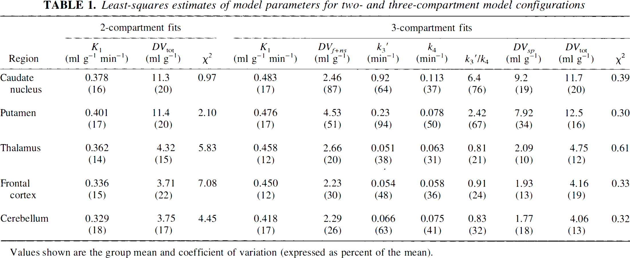
Values shown are the group mean and coefficient of variation (expressed as percent of the mean).

Figure 1 depicts the goodness-of-fit using a two-compartment model estimating K₁, DV_tot and CBV (2C-Fit) and a three-compartment model estimating K₁ k₂′, k₃′, k₄, and CBV (3C-Fit). [¹¹C]DTBZ time-activity curves in putamen (Put) and frontal cortex (FCtx) with 2C (solid lines) and 3C (dashed lines) fits are shown in the top panel. The bottom panel is a plot of the residuals from these fits demonstrating the significantly greater discrepancy between the 2C-Fit and the measured data (solid lines, filled symbols) than the 3C-Fit and the measured data (dashed lines, open symbols).

Fig. 1.

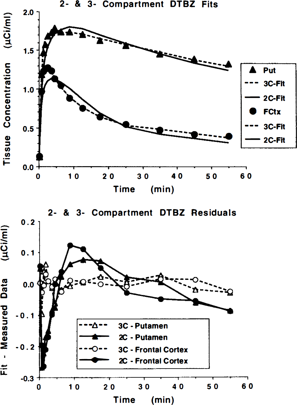
Nonlinear least-squares fits using two- and three-compartment models. The top panel shows VOIs for the putamen (triangles) and frontal cortex (circles) and the least-squares fits using two-compartment (solid curves) and three-compartment (dashed curves), demonstrating the lack of fit of the two-compartment model. The bottom panel shows the residuals of the fits (fitted values - measured data) for the same VOIs. Note the significantly larger residuals for the two-compartment fits (filled symbols) than the three-compartment fits (open symbols).

Figure 2 contrasts the group mean ± 1 SD for four different possible measures of binding density, k₃′, k₃′/k₄, DV_sp, and DV_tot The values for k₃′ have been multiplied by 10 for better viewing. Note that the variability in the measures for k₃′ and k₃′/k₄ are prohibitively high in regions of high binding density, with coefficients of variation exceeding 75%, while variability in regions with lower binding density is much lower, particularly for k₃′/k₄ with coefficients of variation of only 20–30%. Variability in DV estimates is quite consistent across regions with coefficients of variation ranging from 10% to 20%, except of DV_sp in the putamen, which was more highly variable.

Fig. 2.

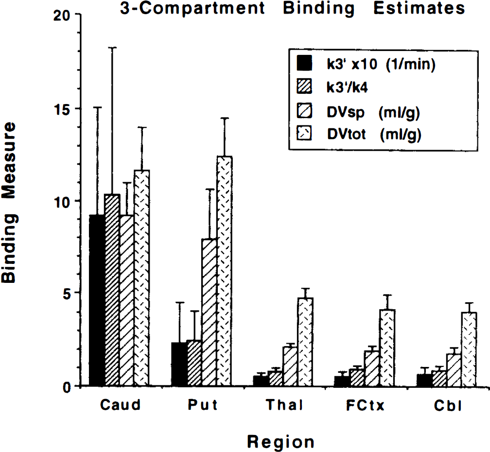
Possible VMAT2 binding indices for three-compartment DTBZ analysis. Given are group mean ± 1 SD for four different potential binding indices (see text for details). Estimates of k₃′ or k₃′/k₄ are very unstable in caudate and putamen. Estimates of DV_sp are quite stable, but note the discrepancy in the relative volumes of specific (DV_sp) and free + nonspecific (DV_tot — DV_sp) compartments between caudate nucleus and putamen.

Table 2 gives results when constraining either DV_f+ns or k₄ in the three-compartment analysis. Results are shown for parameter estimates fitting all rate constants, fixing the free + nonspecific distribution volume to 2.40 ml g⁻¹, and fixing the dissociation rate constant to 0.077 min⁻¹. Fits are reported only for putamen and frontal cortex. Results from fits of the caudate nucleus data were similar to those of the putamen, while results from fits of the thalamus and cerebellar data were similar to those of the frontal cortex.

Table 2.

Effect of constraining DV_f+ns or k₄ on three-compartment model estimations

Region	Model	K₁ (ml g⁻¹ min⁻¹)	DV_f+ns (ml g⁻¹)	k₃′ (min⁻¹)	k₄ (min⁻¹)	k₃/′k₄	DV_sp (ml g⁻¹)	DV_tot (ml g⁻¹)	χ²
Putamen	Fit all	0.476 (17)	4.53 (51)	0.23 (94)	0.078 (50)	2.42(67)	7.92 (34)	12.5 (16)	0.30
	Fixed DV‘	0.496 (17)	2.40 Fixed	0.77 (142)	0.25 (161)	3.34 (24)	8.18 (24)	11.7 (18)	0.46
	Fixed k₄	0.454 (12)	6.19 (42)	0.087 (78)	0.077 Fixed	1.13 (78)	4.85 (38)	12.2 (21)	0.49
Frontal cortex	Fit all	0.450 (12)	2.23 (30)	0.054 (48)	0.058 (36)	0.91 (24)	1.93 (13)	4.16 (19)	0.33
	Fixed DV‘	0.421 (19)	2.40 Fixed	0.042 (90)	0.050 (58)	0.79 (29)	1.94 (29)	4.39 (14)	132
	Fixed k₄	0.456 (11)	2.13 (30)	0.072 (23)	0.077 Fixed	0.93 (23)	1.87 (16)	4.00 (21)	0.58

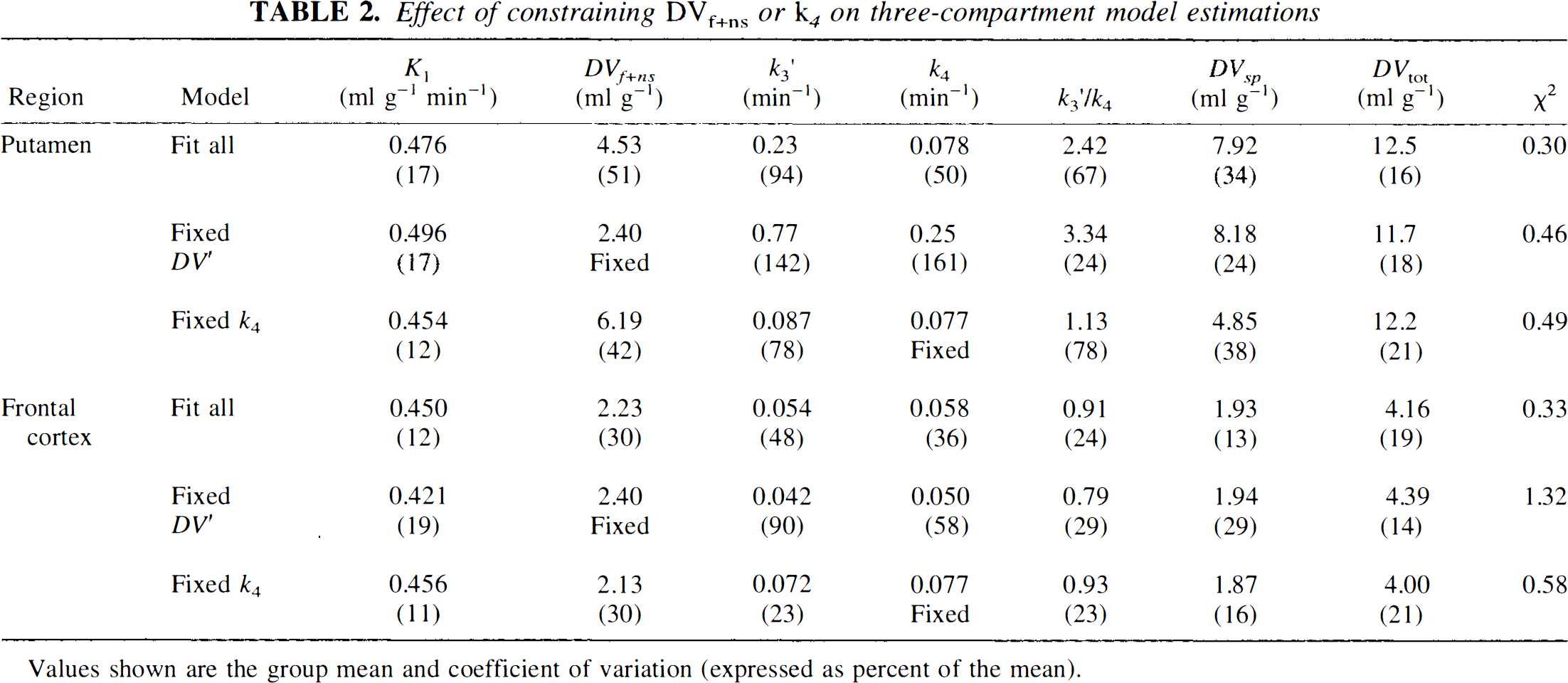
Values shown are the group mean and coefficient of variation (expressed as percent of the mean).

Table 3 shows K₁ and DV_tot estimates obtained from both the two-compartment weighted integral and the Logan plot methods using the VOIs defined for the least-squares analysis. Weighted integral estimates excluded data from the first 30 s to reduce CBV effects. Data from 10 min and later were used for the Logan DV_tot estimate, while the entire data set was used for the determination of K₁. Reported values give the mean and percent coefficient of variation for the group. Figure 3 shows functional images of K₁ (top) and DV_tot (bottom) at three brain levels from a typical subject for the weighted integral (left) and Logan (right) methods of analysis.

Fig. 3.

Parametric images of DTBZ transport and binding. Shown at six brain levels are parametric images of DTBZ BBB transport, K₁ (top) and total distribution volume, DV_tot (bottom) as estimated using a weighted integral approach (left) and the Logan plot graphical analysis (right).

Table 3.

Pixel-by-pixel estimates of model parameters for weighted integral and Logan plot analysis

Region	Weighted Integral		Logan Plots
Region	K₁ (ml g⁻¹ min⁻¹)	DV_tot (ml g⁻¹)	K₁ (ml g⁻¹ min⁻¹)	DV_tot (ml g⁻¹)
Caudate nucleus	0.433 (14)	12.3 (16)	0.410 (15)	11.7 (14)
Putamen	0.472 (17)	12.6 (17)	0.442 (15)	12.2 (14)
Thalamus	0.480 (12)	4.39 (12)	0.410 (13)	4.62 (11)
Frontal cortex	0.450 (12)	3.77 (16)	0.370 (12)	4.03 (14)
Cerebellum	0.407 (17)	3.70 (15)	0.344 (17)	3.86 (13)

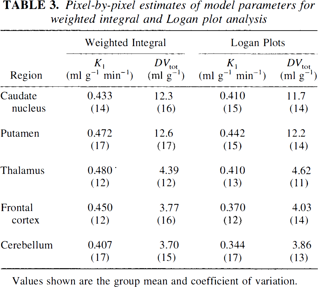
Values shown are the group mean and coefficient of variation.

Figures 4 and 5 present results directly comparing two- and three-compartment nonlinear least-squares VOI analysis with pixel-by-pixel weighted integral and Logan analysis. Figure 4 shows DTBZ binding estimates of DV_tot for each method. Note the extremely similar variability in all DV measurements. Figure 5 shows DTBZ transport rate constant estimates for the four analysis methods. The two-compartment least-squares approach yields the lowest DV_tot estimates, as might be expected, while the weighted integral approach tends to show slightly higher contrast between regions of high and low binding density. The three-compartment least-squares approach and the Logan method yielded the most similar results. The two-compartment least-squares and the Logan analyses yield consistent underestimation of K₁ compared to the three-compartment analysis, primarily due to the insufficiency of the two-compartment model for describing the measured PET time course. Surprisingly, the weighted integral approach, also based on a two-compartment model, yields less biased estimates than the other approaches making a two-compartment assumption.

Fig. 4.

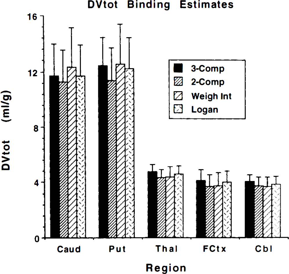
Comparison of four methods for estimating DV_tot. Shown are the group mean ±1 SD (n = 7) for each method. The 3-Comp and 2-Comp values are obtained by nonlinear least-squares estimates from VOI data from three-compartment and two-compartment fits. The Weigh Int and Logan values are obtained from VOIs placed on functional images created by the weighted integral and Logan plot graphical analysis methods, respectively.

Fig. 5.

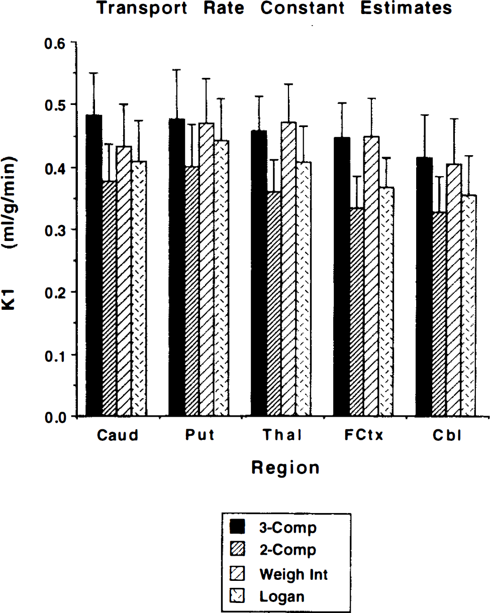
Comparison of four methods for estimating K₁. Shown are the group mean ±1 SD (n = 7) for each method. The 3-Comp, 2-Comp, Weigh Int, and Logan are the same as in Fig. 4.

Besides comparing means and standard deviations for the different measures of binding density, it is important to know the degree of correspondence between the various measures. If two measures are very highly correlated, then they contain nearly same degree of information for distinguishing between levels of binding both from region to region and from subject to subject. Table 4 shows results from linear regression analysis between the various binding or transport parameters for the different analysis methods. In each section of the table correlations are reported to the lower left of the diagonal identity line. Regression slopes and intercepts (in parentheses) are reported to the upper right of the diagonal. For each regression, the parameter in the row heading corresponds to the ordinate, while the parameter from the column heading corresponds to the abscissa. The top third of the table gives results between the various binding measures when the three-compartment analysis is used. While the measures k₃′ and k₃′/k₄ are highly correlated (0.96) due to the relatively stable estimates of k₄, neither of these binding measures correlates very highly with either DV_sp or, particularly, DV_tot. The three-compartment DV_sp and DV_tot estimates are quite highly correlated (0.92) although not nearly as highly as the three-compartment DV_tot correlates with the DV_tot estimates from the other analysis methods (0.994–0.999), as shown in the middle section of the table. Regressions between total distribution volume estimates from three-compartment least-squares analysis (3C DV_tot) and both the three-compartment specific distribution volume estimates (3C DV_sp) (top) and the Logan plot measure of DV_tot (bottom) are shown in Fig. 6. It is evident that for regions with both high and low binding density there is significantly better agreement across subjects between the two DV_tot measures than between DV_tot and DV_sp. The bottom portion of Table 4 gives correlations between K₁ measures for the different methods. These correlations are moderately strong although not as high as between the DV estimates.

Fig. 6.

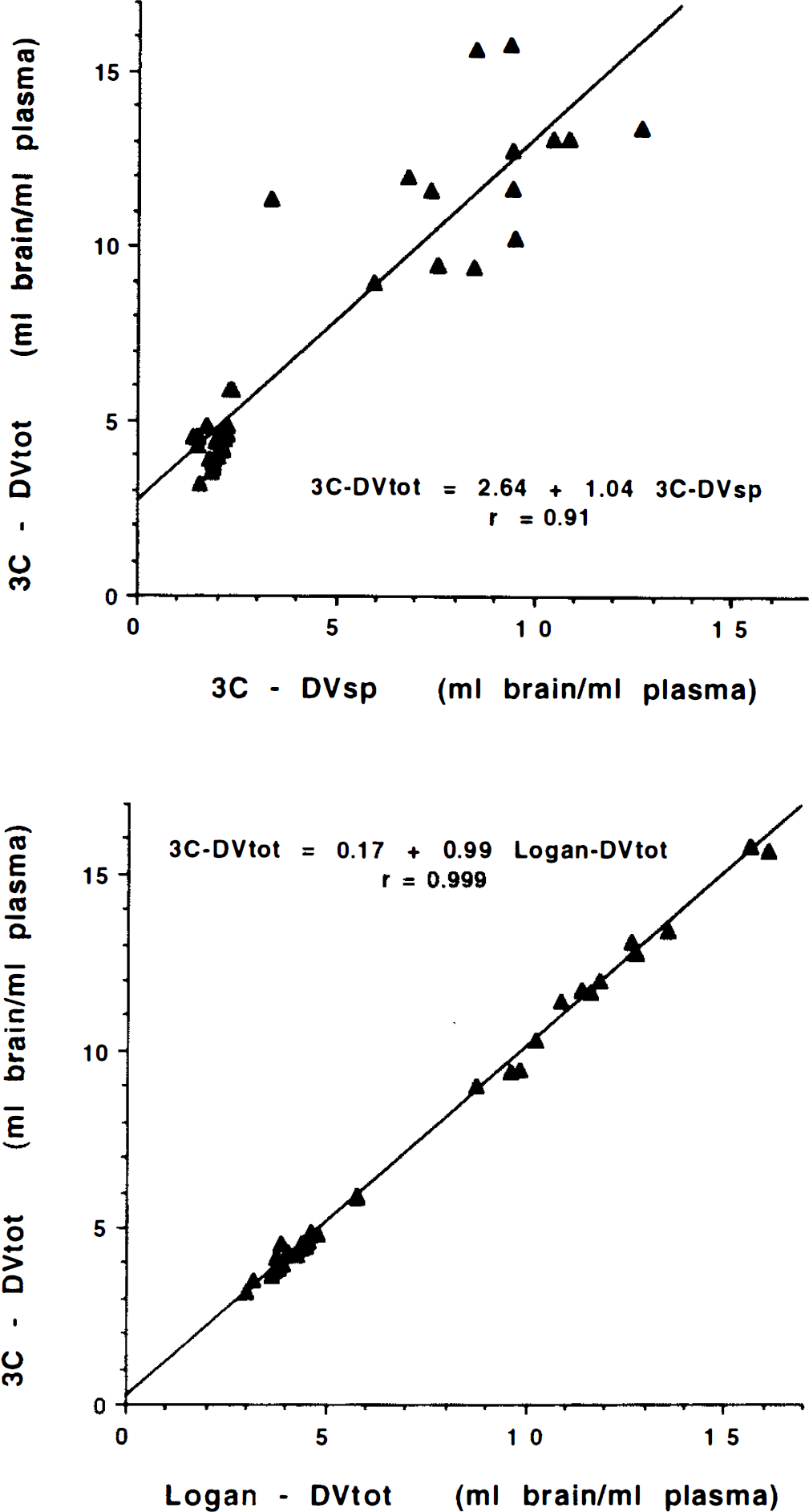
Correlations between binding parameters. Shown in the top panel is the relationship between the three-compartment estimate of DV_tot and the three-compartment estimate of DV_sp. Shown in the bottom panel is the relationship between the three-compartment and Logan plot estimates of DV_tot. Each plot contains data from five regions for each of the seven subjects.

DISCUSSION

In this work we describe methods of analysis of PET studies with (+)-α-[¹¹C]dihydrotetrabenazine (DTBZ) for quantifying levels of binding to the vesicular monoamine transporter. Preliminary pharmacokinetic modeling of the racemic radioligand (±)-α-[¹¹C]DTBZ [where the (–)-isomer has an extremely low 2 μM affinity for the VMAT2 binding site; (Kilbourn et al., 1995)] demonstrated high uncertainties in estimates of k₃′ and k₃′/k₄, moderate uncertainties in DV_tot, and stable estimates of DV_tot (Koeppe et al., 1995a,b; Frey et al., 1995; Gilman et al., 1995). Thus, as in our previous work with [¹¹C]flumazenil, a PET radioligand also demonstrating rapidly reversible binding (Koeppe et al., 1991), we have investigated reductions in the complexity of the compartmental model for [¹¹C]DTBZ, thereby producing a simple estimate for the ligand's tissue distribution volume that might be used as an index of the density of VMAT2 binding sites. In this analysis, we have explored the performance of both pixel-by-pixel estimation procedures capable of producing functional images of the transport and binding parameters and volume-of-interest (VOI) analyses employing nonlinear least-squares optimization, paying particular attention to both the degree of precision and level of bias afforded by each analysis alternative. Based on the present studies, we have chosen a method of analysis that yields an estimate of the total tissue distribution volume (DV_tot) of DTBZ. This approach provides trade-off between bias and precision and provides a method that will optimize our ability to detect differences in the level of DTBZ binding between groups of subjects or between brain regions within a single subject, as well as detect changes in individual subjects over time.

The relative performance of the two- and three-compartment model configurations can be evaluated through comparison of the parameter estimates presented in Table 1. The goodness-of-fit as measured by χ² is significantly better for the three-compartment than the two-compartment model for all regions examined, suggesting that equilibration between tissue compartments is not sufficiently rapid to allow the accurate description of DTBZ kinetics by a two-compartment model. Tissue heterogeneity may also play a role in the lack of fit of the two-compartment model; however, a similar analysis of the tracer [¹¹C]flumazenil (Koeppe et al., 1991) has demonstrated that a two-compartment model does describe the kinetics of that ligand quite well. Therefore, tissue heterogeneity may contribute to, but is not likely to be the major cause of, the lack of fit. Figure 1 also demonstrates these differences in goodness of fit. Note that both regions of high and low binding show biases and lack of fit to a similar degree (solid curves). The variability in the estimates of the total tissue distribution volume DV_tot and transport parameter K₁ are nearly the same for both two- and three-compartment approaches, with coefficients of variation generally ranging from 15% to 20% across regions. However, due to lack of goodness of fit, both parameters are significantly biased in the two-compartment estimation with the 2C DV_tot being underestimated by an average of ˜8% across all subjects (paired t value = 8.9, p < 0.0001) and the 2C K₁ underestimated by 21% on average (paired t value = 15.3, p < 0.0001). It is interesting to note that the propagation of error due to lack of fit is seen to a considerably greater extent in K₁ than DV_tot The degree of variability in the absolute values of DV_tot and K values for [¹¹C]DTBZ is very typical of the most commonly used successful PET tracers.

The precision in the estimates of the various parameters or combinations of parameters from the three-compartment model that reflect binding density varied considerably (Fig. 2). Estimates of the parameter k₃′ were highly variable, particularly in the regions of high binding density—caudate nucleus and putamen. Estimates of k₄ were somewhat more stable and positively correlated with k₃, and thus the ratio k₃′/k₄ is a little less variable. Estimates of DV_sp, which is equivalent to DV_f+ns(k₃′/k₄), are significantly more stable, particularly in regions of lower binding density such as cortex, thalamus, and cerebellum. This is caused by a strong positive correlation between parameters k₂′ and k₃ in the estimation procedure (noting DV_f+ns is proportional to 1/k₂′). As discussed in the theory section, under ideal conditions we would select either of the measures k₃ or k₃/k₄ as our index of binding density because they vary directly with B_max′ (linear with zero intercept and unit slope). If using these measures is not feasible (i.e., due to high estimation uncertainty), then an estimate of DV_sp would be preferable (linear with zero intercept but slope of DV_f), and finally DV_tot (linear but with slope of DV_f and intercept of DV_f+ns). However, as we have noted with these DTBZ data, reduction in bias, when progressing from DV_tot to DV_sp to either k₃/k₄ or k₃, occurs with a concomitant loss of precision. This is due to the inability of the kinetic analysis to consistently distinguish between the relative sizes of the free + nonspecific and bound compartments even when the total distribution volume is estimated with high precision. Since estimates of k₂′ and k₃ are highly positively correlated, a single fit tends to either overestimate or underestimate both parameters. A fit overestimating both k₂ and k₃ underestimates the free + nonspecific pool (since K₁/k₂′ is small) and overestimates the bound pool (since k₃′/k₄ is large). Conversely, a fit underestimating both k₂ and k₃ yields the opposite result. This problem with parameter identifiability becomes more pronounced with higher rates of binding relative to BBB transport (Koeppe et al., 1990, 1994), thus explaining the poorer precision of DV_sp, k₃′/k₄, and k₃′ estimates for caudate and putamen than for thalamus, cortex, and cerebellum as demonstrated in Table 1 and Fig. 2.

Data in the top section of Table 4 also point to these difficulties. The parameters k₃′ and k₃′/k₄ correlate highly, yet neither parameter correlates highly with either DV_sp or DV_tot. Furthermore, the relationship between DV_sp and DV_tot (Fig. 6, top) shows a moderately high correlation (0.92) and regression parameters are close to the expected slope equal to one (1.04) and intercept equal to DV_f+ns (2.6).

Table 4.

Regression analysis of binding and transport measures across methods^a

	DV _tot	DV_sp	k₃′/k₄	k₃′
Binding estimates3-comp analysis
DV _tot	—	1.04 (2.6)	0.66(4.1)	9.1(4.3)
DV_sp	0.92	—	0.70 (2.2)	7.1 (2.3)
k ₃ ₄	0.46	0.70	—	11.3(0.10)
k ₃	0.52	0.75	0.96	—
	3-Comp	2-Comp	Logan	Weight Int
DV_tot estimates
3-Comp	—	1.03(0.30)	0.99(0.16)	0.89 (0.86)
2-Comp	0.997	—	0.96 (−0.11)	0.86(0.53)
Logan	0.999	0.998	—	0.90 (0.69)
Weight Int	0.994	0.998	0.996	—
	3-Comp	2-Comp	Logan	Weight Int
K₁ estimates
3-Comp	—	1.20(0.05)	1.08(0.04)	1.01 (0.01)
2-Comp	0.84	—	0.95(0.01)	0.88 (−0.04)
Logan	0.86	0.97	—	0.95 (−0.03)
Weight Int	0.72	0.79	0.79	—

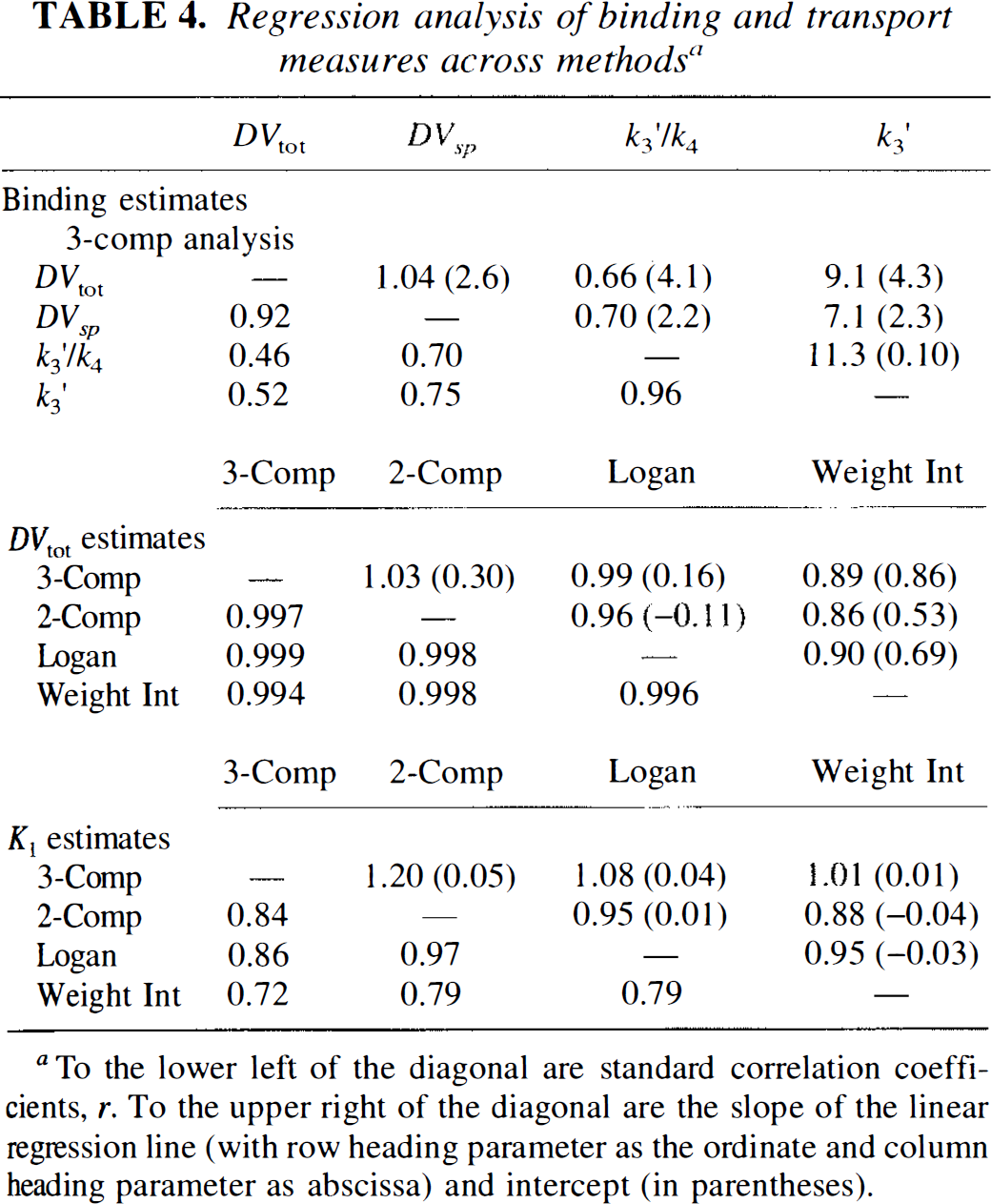
To the lower left of the diagonal are standard correlation coefficients, r. To the upper right of the diagonal are the slope of the linear regression line (with row heading parameter as the ordinate and column heading parameter as abscissa) and intercept (in parentheses).

We explored analyses with two other model configurations in an attempt to improve precision in the estimates of the binding indices k₃, k₃/k₄, and DV_sp with the goal of using one of these measures of binding in order to avoid the inherent bias from free and nonspecific binding when using DV_tot as the index of binding density. In one configuration, the value of DV_f+ns was fixed to the population mean across nonstriatal regions, while in the second alternative, the value of k₄ was fixed to the population mean across all regions. Goodness-of-fit measures were significantly poorer when DV_f+ns was fixed (to 2.40) than when fitted. Precision in estimates of DV_sp, however, was not improved by fixing DV_f+ns. Since DV_tot is the sum of DV_f+ns and DV_sp, equivalent results are obtained by estimating the DV_tot with the unconstrained model and simply subtracting of the fixed value for DV_f+ns to yield DV_sp.

The results when using a fixed value for k₄ differed between regions of high and low binding. In regions of low binding (i.e., thalamus, cortex, and cerebellum) results were very similar to results when fitting k₄. This was not totally unexpected since the uncertainty in k₄ was reasonably low even when fitted, and thus the variability in the estimates of k₃′ and k₃′/k₄ were not substantially different. The result of fixing k₄ when fitting regions of high binding was that the estimation procedure was still unable to accurately determine the relative sizes free + nonspecific and specific pools. As with the full fit, DV_tot was estimated with good precision, but for some subjects the free + nonspecific pool was estimated as having the larger component, while in others, the specific pool was estimated as larger. Thus, the constraint of k₄ yielded binding estimates with neither improved precision nor less bias.

Both the weighted integral and the graphical methods produce functional images for ligand transport and binding of high image quality (Fig. 3). The DV_tot images appear very similar; however, those produced by the graphical approach show slightly less noise than those from the weighted integral approach, particularly in areas of high binding. In these areas, the clearance from brain is slower and the precision of the weighted integration method decreases. The contrast between areas of high and low binding is slightly lower for the graphical approach than it is for the weighted integral method, but is in better agreement with the three-compartment least-squares estimates (Table 4, Fig. 6). The transport images also appear similar, but with lower global values for the graphical approach than for the weighted integral method. The inherent assumptions made of the two methods are different. The weighted integral approach is based on a two-compartment model, which assumes rapid equilibration between bound and free + nonspecific compartments. The least-squares fits presented in Fig. 1 show that this assumption is not fully justified, and therefore a certain level of bias will propagate into the transport and binding estimates. Although the two-compartment least-squares approach makes this same assumption, the magnitude of the biases that propagate into the transport and binding estimates may differ between analysis methods. The graphical approach of Logan has the advantage for estimation of DV_tot that no assumption is required concerning the rate of equilibration. As pointed out by Logan, if a two-compartment model is justified, then the plot becomes linear immediately with slope = DV_tot and intercept = −1/k₂ (ignoring blood volume) while the plot for a three- (or more) compartment model becomes linear only as all compartments approach equilibrium. DV_tot is still accurately reflected by the linear portion of the plot; however, no simple mathematical description for the intercept remains. Simulated noise-free DTBZ time-activity curves were generated and used to determine the optimal time intervals to use in the graphical analysis. The Logan plots for both the simulated and actual DTBZ data became nearly linear for all regions by approximately 10 min after injection. DV_tot is progressively underestimated as earlier data is included, reaching 10% when using all the data. Simulations showed that when DV_tot was estimated from data 10 min and later, underestimates never exceeded 3%. If even more early data are excluded, this last 3% bias can be removed, but at the expense of increased noise propagation and thus a 10-min starting time was selected for all analyses. Unlike estimates of DV_tot, estimates of K₁ (slope/-intercept), becomes more biased when early data is omitted. Thus, a separate Logan plot calculation including all the data was selected for estimating K₁.

The regional estimates of DV_tot and K₁ for the two-and three-compartment nonlinear least-squares fits plus the two pixel-by-pixel analyses discussed in the preceding paragraph are compared in Figs. 4 and 5, respectively. All four approaches yield estimates with essentially the same coefficients of variation. The two-compartment estimations yield consistent underestimations of DV_tot relative to three-compartment estimations. Weighted integral analysis results in slightly higher contrast between regions of high and low binding than do the other methods. This is due to the inherent difference in how biases caused by noninstantaneous equilibration between compartments propagate into the DV_tot estimate. DV_tot estimates from the graphical method are in closest agreement with three-compartment estimates. Even though the group means are slightly different for the different methods, these differences are very consistent across the brain and from subject to subject (Table 4, middle section, and Fig. 6). The correlations between any two methods never fell below 0.994. The contrast enhancement of the weighted integral approach is reflected by the nonunity slopes (0.86–0.90) of the regressions against the other methods.

The two-compartment and graphical K₁ estimates are consistently lower than those from three-compartment or weighted integral estimation. Failure of free + nonspecific and bound compartments to instantaneously equilibrate caused an expected underestimation of K₁; however, it was somewhat surprising that the weighted integral method, making the same equilibration assumption, did not yield substantially biased K₁ estimates. Correlations between methods are lower for K₁ than for DV_tot (Table 4, bottom), ranging from 0.72 to 0.97. These lower correlations are caused mostly by the more limited range of values across regions for K₁ compared to DV_tot, but also in part by the differences in how CBF and time shift are accounted for between methods. In addition, because the errors due to the lack of instantaneous equilibration are most apparent in the early phase of the scan and since K₁ is determined largely by the data acquired at early times after injection, these errors will affect estimates of K₁ to a greater extent than DV_tot.

These results strongly suggest the use of a three-compartment model configuration for VOI analysis. For functional imaging, the graphical approach of Logan appears slightly superior to weighted integral analysis for the estimation of DV_tot yielding less noisy images and results that are closer to those from three-compartment estimations. The weighted integral method, however, appears slightly superior for estimating K₁.

In summary, we have evaluated two- and three-compartment model configurations for kinetic analysis of the monoamine vesicular transporter marker (+)-α-[¹¹C]DTBZ. A three-compartment model was found to provide significantly better fits to the data than a two-compartment model. Estimates of the parameter k₃ or the ratio k₃/k₄ (= B_max′/K_d) from the three-compartment configuration were too highly variable to be used reliably as the measure of binding density, particularly for the high binding regions of the basal ganglia. Estimates of the distribution volume of the specific compartment (DV_sp) were considerably more stable, yet the kinetic analysis was still not able to consistently determine the relative volumes of free + nonspecific and specific binding compartments for those regions with high binding density. We conclude that a measure of the total distribution volume, which can be estimated with high precision, provides an index of VMAT2 binding density with the greatest reliability. Since the increase in precision of the total distribution volume is greater than the decrease in the dynamic range of this measure, we believe that DV_tot will provide the most sensitive index of change in VMAT2 density and the best power for discriminating binding levels between different groups of subjects, although studies inpatient populations are required to confirm this prediction. We have also shown that simple pixel-by-pixel methods yield estimates of DV_tot that correlate extremely highly with the three-compartment nonlinear least-squares analysis and thus can be used with confidence to produce functional images of ligand BBB transport in addition to vesicular monoamine transporter binding density. We thus feel our quantitative estimates of VMAT2, represented by the DV_tot for [¹¹C]DTBZ, provide a new and valuable option to the determination of dopaminergic terminal losses in neurodegenerative disease.

Footnotes

Abbreviations used

Acknowledgment:

This work was supported in part by the Department of Energy grant DE-FG02-87ER60561 and the National Institutes of Health grant P01 NS-15655 and ROI MH-47611. The authors would like to thank the PET radiochemistry and technologist staff of the Division of Nuclear Medicine for production of isotopes and acquisition of PET data.

References

Alpert

Eriksson

Chang

Bergstrom

Litton

Correia

Bohm

Ackermann

Taveras

(1984) Strategy for the measurement of regional cerebral blood flow using short-lived tracers and emission tomography. J Cereb Blood Flow Metab 4: 28–34.

Aquilonius

S-M

Bergstrom

Eckernas

S-A

Hartvig

Leenders

Lundquist

Antoni

Gee

Rimland

Uhlin

Langstrom

(1987) In vivo evaluation of striatal dopamine reuptake sites using 11C-nomifensine and positron emission tomography. Acta Neurol Scand 76:283–287.

Bevington

(1969) Data Reduction and Error Analysis for the Physical Sciences, New York, McGraw-Hill, pp 232–241.

DaSilva

Kilbourn

(1992) In vivo binding of [11C]tetrabenazine to vesicular monoamine transporters in mouse brain. Life Sci 51: 593–600.

DeJesus

Holden

Endres

Shelton

Nickles

(1995) Comparison of four [F-18]-labeled analogs as PET imaging agents for dopamine nerve terminals. J Nucl Med 36:253P.

Frey

Koeppe

Mulholland

Jewett

Hichwa

Ehreukaufer

RLE

Carey

Welland

Kohl

Agranoff

(1992) In vivo muscarinic cholinergic receptor imaging in human brain with [11C] scopolamine and positron emission tomography. J Cereb Blood Flow Metab 12:147–154.

Frey

Koeppe

Kilbourn

Vander Borght

Albin

Gilman

Kuhl

(1995) Reduction of presynaptic monoaminergic vesicles in the striata of Parkinsonian patients and in normal human aging. J Cereb Blood Flow Metab 15(1):S38.

Frost

Rosier

Reich

Smith

Ehlers

Snyder

Ravert

Dannais

(1993) Positron emission tomographic imaging of the dopamine transporter with 11C-WIN 35,428 reveals marked declines in mild Parkinson's disease. Ann Neurol 34:423–431.

Garnett

Firnau

Nahmias

(1983) Dopamine visualized in the basal ganglia of living man. Nature 305:137–138.

10.

Gjedde

Reith

Dyve

Leger

Guttman

Diksic

Evans

Kuwabara

(1991) Dopa decarboxylase activity of the living human brain. Proc Natl Acad Sci USA 88:2721–2725.

11.

Gjedde

Leger

Cumming

Yasuhara

Evans

Guttman

Kuwabara

(1993) Striatal L-DOPA-decarboxylase activity in Parkinson's disease in vivo: Implications for the regulation of dopamine synthesis. J Neurochem 61:1,538–1,541.

12.

Gilman

Frey

Koeppe

Junck

Little

Vander Borght

Lohman

Martorello

Lee

Jewett

Kilbourn

(1995) Decreased striatal monoaminergic presynaptic terminals in OPCA and MSA demonstrated with [11C]dihydrotetrabenazine and PET. J Cereb Blood Flow Metab 15(1):S752.

13.

Hadjiconstantinou

Wemlinger

Silvia

Hubble

Neff

(1993) Aromatic L-amino acid decarboxylase activity of mouse striatum is modulated via dopamine receptor. J Neurochem 60:2,175–2,180.

14.

Henry

J-P

Scherman

(1989) Radioligands of the vesicular monoamine transporter and their use as markers of monoamine storage vesicles. Biochem Pharmacol 38:2,395–2,404.

15.

Huang

Barrio

Grafton

Melega

Hoffman

Satyamurthy

Mazziotta

Phelps

(1991) Kinetics and modeling of L-6-[18F]fluoro-DOPA in human positron emission tomographic studies. J Cereb Blood Flow Metab 11:898–913.

16.

Ikegami

Prasad

(1990) Neuropeptide-dopamine interactions. V. Cyclo(His-Pro) regulation of striatal dopamine transporter complex. Peptides 11:145–148.

17.

Innis

Seibyl

Scanley

Laruelle

Abi-Dargham

Wallace

Zea-Ponce

Zoghbi

Wang

Gao

Neumeyer

Charney

Hoffer

Marek

(1993) SPECT imaging demonstrates loss of striatal transporters in Parkinson's disease. Proc Natl Acad Sci USA 90:11,965–11,969.

18.

Kilbourn

(1994) PET radioligands for vesicular neurotransmitter transporters. Med Chem Res 5:113–126.

19.

Kilbourn

Sherman

Pisani

(1992) Repeated reserpine administration reduces in vivo [18F]GBR-13119 binding to the dopamine uptake site. Eur J Pharmacol 216:109–112.

20.

Kilbourn

Lee

Vander Borght

Jewett

Frey

(1995) Binding of α-dihydrotetrabenazine to the vesicular monoamine transporter is stereospecific. Eur J Pharmacol 278:249–252.

21.

Kish

Robaitaille

El-Awar

Clark

Schut

Ball

Young

Currier

Shannak

(1992) Striatal monoamine neurotransmitters and metabolites in dominantly inherited olivopontocerebellar atrophy. Neurology 42(8): 1,573–1,577.

22.

Koeppe

(1990) Compartmental modeling alternatives for kinetic analysis of PET neurotransmitter/receptor studies. In: Frontiers in Nuclear Medicine: In Vivo Imaging of Neurotransmitter Functions in Brain, Heart, and Tumors, ( Kuhl

ed), Washington, DC, American College of Nuclear Physicians, pp 113–139.

23.

Koeppe

Hutchins

Rothley

Hichwa

(1987) Examination of assumptions for local cerebral blood flow studies in PET. J Nucl Med 28:1,695–1,703.

24.

Koeppe

Kilbourn

Frey

Penney

Haka

Kuhl

(1990) Imaging and kinetic modeling of [F-18]GBR 12909 a dopamine uptake inhibitor. J Nucl Med 31:720.

25.

Koeppe

Holthoff

Frey

Kilbourn

Kuhl

(1991) Compartmental analysis of [11C]flumazenil kinetics for the estimation of ligand transport rate and receptor distribution using positron emission tomography. J Cereb Blood Flow Metab 11:735–744.

26.

Koeppe

Frey

Mulholland

Kilbourn

Buck

Lee

Kuhl

(1994) [11C]Tropanyl benzilate binding to muscarinic cholinergic receptors: Methodology and kinetic modeling alternatives. J Cereb Blood Flow Metab 14:85–99.

27.

Koeppe

Frey

Vander Borght

Kilbourn

Jewett

Lee

Kuhl

(1995a) Kinetic evaluation of [C-11]dihydrotetrabenazine (DTBZ) by dynamic PET: A marker for the vesicular monoamine transporter. J Cereb Blood Flow Metab 15(1):S651.

28.

Koeppe

Frey

Vander Borght

Kilbourn

Jewett

Lee

Kuhl

(1995b) Kinetic evaluation of α-[C-11]dihydrotetrabenazine (DTBZ): A PET ligand for assessing the vesicular monoamine transporter. J Nucl Med 36:118P.

29.

Laruelle

Wallace

Seibyl

Baldwin

Zea-Ponce

Zoghbi

Neumeyer

Charney

Hoffer

Innis

(1994) Graphical, kinetic and equilibrium analyses of in vivo [123I]ß-CIT binding to dopamine transporters in healthy human subjects. J Cereb Blood Flow Metab 14:982–994.

30.

Masuo

Pelaprat

Scherman

Rostene

(1990) [3H]Dihydrotetrabenazine, a new marker for the visualization of dopaminergic denervation in the rat striatum. Neurosci Lett 114:45–50.

31.

Mintun

Raichle

Kilbourn

Wooten

Welch

(1984) A quantitative model for the in vivo assessment of drug binding sites with positron emission tomography. Ann Neurol 15:217–227.

32.

Naudon

Leroux-Nicollet

Costentin

(1994) Short-term treatments with haloperidol or bromocriptine do not alter the density of the monoamine vesicular transporter in the substantia nigra. Neurosci Lett 173:1–4.

33.

Near

(1986) [3H]Dihydrotetrabenazine binding to bovine striatal synaptic vesicles. Mol Pharmacol 30:252–257.

34.

Salmon

Brooks

Leenders

(1990) A two-compartment description and kinetic procedure for measuring regional cerebral [11C]Nomifensine uptake using positron emission tomography. J Cereb Blood Flow Metab 10:307–316.

35.

Scherman

Raisman

Ploska

Agid

(1988) [3H]Dihydrotetrabenazine, a new in vitro monoaminergic probe for human brain. J Neurochem 50:1,131–1,136.

36.

Sharpe

Pilotte

Mitchell

De Souza

(1991) Withdrawal of repeated cocaine decreases autoradiographic [3H]mazindollabelling of dopamine transporter in rat nucleus accumbens. Eur J Pharmacol 203:141–144.

37.

Vander Borght

Kilbourn

Desmond

Kuhl

Frey

(1995a) The vesicular monoamine transporter is not regulated by dopaminergic drug treatments. Eur J Pharmacol 294:577–583.

38.

Vander Borght

Sima

AAF

Kilbourn

Desmond

Frey

(1995b) [3H]Methoxytetrabenazine: A high specific activity ligand for estimating monoaminergic neuronal integrity. Neuroscience 68:955–962.

39.

Wiener

Hashim

Lajtha

Sershen

(1989) Chronic L-deprenyl induced up-regulation of the dopamine uptake carrier. Eur J Pharmacol 163:191–194.

40.

Wilson

Nobrega

Carroll

Niznick

Shannak

Lac

Pristupa

Dixon

Kish

(1994) Heterogeneous subregional binding patterns of 3H-WIN 35,428 and 3H-GBR-12,935 are differentially regulated by chronic cocaine self-administration. J Neurosci 14:2,966–2,979.

41.

Wilson

Kish

(1996) The vesicular monoamine transporter, in contrast to the dopamine transporter, is not altered by chronic cocaine self-administration in the rat. J Neurosci 16:3,507–3,510.

42.

Zhu

Juorio

Paterson

Boulton

(1992) Regulation of aromatic L-amino acid decarboxylase by dopamine receptors in the rat brain. J Neurochem 58:636–64.

Kinetic Evaluation of [ 11 C]Dihydrotetrabenazine by Dynamic PET: Measurement of Vesicular Monoamine Transporter

Abstract

Keywords

THEORY

MATERIALS AND METHODS

RESULTS

DISCUSSION

Footnotes

Abbreviations used

Acknowledgment:

References