Optimal Location for Arterial Input Function Measurements near the Middle Cerebral Artery in First-Pass Perfusion MRI

Abstract

One of the main difficulties in obtaining quantitative perfusion values from dynamic susceptibility contrast-magnetic resonance imaging is a correct arterial input function (AIF) measurement, as partial volume effects can lead to an erroneous shape and amplitude of the AIF. Cerebral blood flow and volume scale linearly with the area under the AIF, but shape changes of the AIF can lead to large, nonlinear errors. Current manual and automated AIF selection procedures do not guarantee the exclusion of partial volume effects from AIF measurements. This study uses a numerical model, validated by phantom experiments, for predicting the optimal location for AIF measurements in the vicinity of the middle cerebral artery (MCA). Three different sequences were investigated and evaluated on a voxel-by-voxel basis by comparison with the ground truth. Subsequently, the predictions were evaluated in an in vivo example. The findings are fourfold: AIF measurements should be performed in voxels completely outside the artery, here a linear relation should be assumed between ΔR*₂ and the concentration contrast agent, the exact optimal location differs per acquisition type, and voxels including a small MCA yield also correct AIF measurements for segmented echo planar imaging when a short echo time was used.

Introduction

Perfusion-weighted imaging can provide important physiologic parameters related to the cerebral microvasculature, parameters such as cerebral blood flow (CBF), cerebral blood volume (CBV), mean transit time (MTT), and time of arrival (Ostergaard et al, 1996; Rempp et al, 1994). These parameters enable the identification and characterization of pathologic areas in brain tissue. Perfusion-weighted imaging can identify tissue at risk of infarction in stroke patients, facilitate grading and delineation of brain tumors, and can provide important hemodynamic information in, for example, Alzheimer's disease, obstructive cerebrovascular disease and migraine (Hakyemez et al, 2006; Harris et al, 1998; Kluytmans et al, 1998; Sorensen et al, 1999).

Dynamic susceptibility contrast-magnetic resonance imaging (DSC-MRI) measures brain perfusion by monitoring dynamically the first pass of a bolus of contrast agent through the microvasculature of the brain tissue. Because the concentration of the contrast agent passing through the tissue microvasculature increases, the transverse relaxation time decreases leading to decreased signal magnitude. An arterial input function (AIF), which describes the concentration of the contrast agent passing through an artery feeding the brain, is required for deconvolution to calculate the perfusion parameters CBV (area under the curve of the impulse response or residue function) and CBF (the peak height of the impulse response). The MTT is the ratio of CBV over CBF. An erroneous measurement of the area under the AIF, would not affect the quantitative value of the MTT, because both CBV and CBF scale equally with the area under the AIF. Therefore, it is sufficient to measure the correct shape of the AIF for MTT quantification. However, for correct quantification of CBF and CBV it is necessary to measure the AIF with both a correct shape and a correct peak height (Calamante et al, 2000; Ostergaard et al, 1996).

Although both the magnitude and phase of the DSC-MRI signal can be used for AIF measurements (Akbudak and Conturo, 1996; Perman et al, 1992; Kotys et al, 2007), the magnitude of the signal is used most often. Voxels for the AIF are normally selected either manually (Sorensen et al, 1999) or automatically (Carroll et al, 2003; Mouridsen et al, 2006).

Most automatic and manual AIF selection methods are based on criteria, such as an early rise, small width, high peak height, and large area under the curve. It is known that partial volume effects can affect both the shape and peak height of the measured AIF, thereby leading to large quantification errors of CBF and CBV (van Osch et al, 2005). Because these effects can also lead to more narrow curves or a higher maximum value, most selection procedures do not prohibit the inclusion of voxels that exhibit partial volume effects. For parallel-orientated arteries, such as the internal carotid artery, partial volume errors (PVEs) can be corrected (van Osch et al, 2003a), but in normal clinical practice the AIF is measured in the vicinity of the middle cerebral artery (MCA) because of its size and location close to brain tissue. Because the MCA is oriented approximately perpendicular to the main magnetic field, correction for PVEs is not possible and distortions of the AIF can occur. A good theoretical basis for the proper criteria to select the optimum location to measure the AIF (e.g. exhibiting the correct shape and height) in the vicinity of the MCA is currently lacking.

The goal of this study is to provide a theoretical basis for AIF selection close to the MCA, using a numerical model validated using phantom experiments. The optimal location for selecting the AIF in the vicinity of the MCA was identified for several different types of gradient echo sequences that are commonly used in DSC-MRI. Furthermore, the findings were tested in a clinical example of a patient who was scanned twice with different DSC-MRI sequences.

Materials and methods

The aim of this study is to find the optimal location for AIF selection in the vicinity of the MCA. For this purpose, a numerical model was developed that included both image formation and the dependence of the relaxation time and magnetic field distribution on the presence of contrast agent. Three commonly used DSC-MRI sequences, single-shot echo planar imaging (EPI), dual echo-segmented EPI and PRESTO (Principles of echo-shifting with a train of observations) (Liu et al, 1993), were implemented in the numerical model and the model was validated by phantom experiments.

After validation using parameters representative for the experimental setup, the model was adjusted to resemble in vivo AIF measurements more closely: the passage of contrast agent through brain tissue surrounding the artery was included and relaxation rates and values were changed to in vivo values. This extended model will be referred to as the advanced model. The diameter of the vessel was varied in the advanced model to study the influence of the size of the MCA on the AIF measurements.

Numerical Model

The MCA in the numerical model was modeled as an infinite cylinder perpendicular to the main magnetic field and parallel to the left and right axes. The reported diameter of the MCA varies from 2 to 4mm (Monson et al, 2005; Serrador et al, 2000) and the average flow in the MCA is 2.6 mL/sec (van Osch et al, 2006). For reasons of symmetry, only the plane whose normal is parallel to the vessel axis needs to be considered in the simulations. All results are therefore presented in a sagittal view, although the model represents acquisition of transverse slices.

Contrast agent properties: Gadolinium-based contrast agents (e.g. Gd-DTPA) affect magnetic susceptibility (Δχ=dχ· [Gd], with dχ = 0.3209 × 10⁻³ (L/mol) at 1.5T (van Osch et al, 2003a)), as well as longitudinal and transverse relaxation times. The dependence of the transverse relaxation rate on the concentration of Gd-DTPA is different for aqueous solutions, as used in the phantom experiments; and for whole blood, where the presence of red blood cells causes a quadratic relation between transverse relaxation rate and contrast agent concentration (Akbudak et al, 1998). Therefore, a linear relation between the transverse relaxation rate and concentration Gd-DTPA was used for comparisons with phantom experiments (5.3 and 5.2 L/mmol/sec at 1.5 and 3T, respectively (Pintaske et al, 2006)). For the advanced model a quadratic relation between transversal relaxation rate of intravascular blood and concentration of Gd-DTPA was used (linear term 7.62 L/mmol/sec; quadratic term 0.57 L²/mmol²/sec at 1.5T; van Osch et al, 2003a). When modeling the passage of contrast agent through the microvasculature of tissue a linear relation was used (44 and 88 L/mmol/sec at 1.5 and 3T; Kjolby et al, 2006). The effect of the contrast agent on the longitudinal relaxation was only taken into account for the tissue passage by assuming a single longitudinal relaxation rate for the tissue and microvascular components combined and by assuming an intact blood–brain barrier (4.3 and 3.3 L/mmol/sec at 1.5 and 3T (Morkenborg et al, 1998; Pintaske et al, 2006)). T₁ effects inside the MCA were assumed negligible, because these will be minimal for relatively long repetition times because of inflow of fresh spins (Calamante et al, 2007).

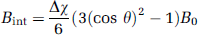
Magnetic field changes: An intravascular susceptibility change in a vessel perpendicular to the main magnetic field results in local field changes in and around the vessel. These local field changes were calculated using Maxwell equations taking into account the sphere of Lorenz (Haacke, 1999):

$$B_{\text{int}}=\frac{\Delta \chi }{6}(3(\text{cos}\theta {)}^2-1)B_0$$

(1)

$$B_{\text{ext}}=(\frac{\Delta \chi }{2}{\left(\frac{a}{\rho }\right)}^2(\text{sin}\theta {)}^2\text{cos}2\phi )B_0$$

(2)

with B_int the magnetic field change inside the vessel, B_ext the magnetic field change outside the vessel, B₀ the main magnetic field strength, Δχ the susceptibility difference between the intra- and extravascular compartment, a the radius of the vessel, ρ, θ, and φ spherical coordinates where ρ equals the distance from the grid point to the vessel center and θ the angle between the vessel and the main magnetic field B₀ (assumed to be 90° for the MCA). In the absence of contrast agent, it was assumed that there is no susceptibility difference between the interior and exterior of the MCA.

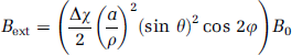
Image formation: Local magnetic field changes lead to distortions in MR images, especially when using fast imaging techniques such as EPI. Such image distortions were included in the model by simulating the image formation process. Frequency encoding was assumed parallel to the MCA. Imaging for EPI and segmented EPI was modeled using the expression:

$$\begin{array}{rl}& S(k_m,z_i,[\text{Gd}])=\\ & \sum _{j=1}^N{M}_0\cdot \frac{\text{sin}\alpha \cdot (1-\text{exp}(-\frac{\text{TR}}{T_1(x_j,z_i,[\text{Gd}])}))}{(1-\text{cos}\alpha \cdot \text{exp}(-\frac{\text{TR}}{T_1(x_j,z_i,[\text{Gd}])}))}\cdot \text{exp}(-\frac{T_m}{T_2^{\ast }(x_j,z_i,[\text{Gd}])})\cdots \\ & \text{exp}(i\cdot 2\cdot \pi \cdot k_m\cdot x_j)\cdot \text{exp}(i\cdot \gamma \cdot \Delta B(x_j,z_i,[\text{Gd}])\cdot T_m)\end{array}$$

(3)

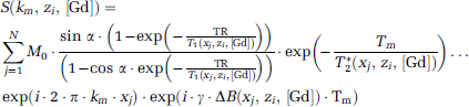
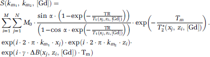
with M₀ the initial longitudinal magnetization, α the flip angle, TR the repetition time, T¹ the longitudinal relaxation (1.5T: 0.95, 1.2, and 1.4 secs for tissue, MnCl₂-doped water and blood (Pedersen et al, 2004) and 3.0 T: 1.1 and 1.7 secs for tissue and blood (Golay et al, 2005; Lu et al, 2004)), T_m the time from excitation to readout of each k-line (the time between each k-line (ΔT_m) is 0.74 and 0.97 ms, for EPI and segmented EPI, respectively), T*₂ is 0.1 sec at 1.5 T for tissue (Pedersen et al, 2004), MnCl₂-doped water and blood and 0.07 sec at 3.0 T for tissue, k_m the mth k-line, x the position within the slice, and γ is the gyromagnetic ratio. Equation (3) is similar to that of Duhamel et al (2006). Imaging parameters were taken from local perfusion protocols and were equal to the imaging parameters of the phantom experiments. Because PRESTO is commonly used as 3D sequence, Equation (3) is extended to two-phase encoding directions:

$$\begin{array}{rl}& S(k_{m_1},k_{m_2},[\text{Gd}])=\\ & \sum _{i=1}^M\sum _{j=1}^N{M}_0\cdot \frac{\text{sin}\alpha \cdot (1-\text{exp}(-\frac{\text{TR}}{T_1(x_j,z_i,[\text{Gd}])}))}{(1-\text{cos}\alpha \cdot \text{exp}(-\frac{\text{TR}}{T_1(x_j,z_i,[\text{Gd}])}))}\cdot \text{exp}(-\frac{T_m}{T_2^{\ast }(x_j,z_i,[\text{Gd}])})\cdots \\ & \text{exp}(i\cdot 2\cdot \pi \cdot k_{m_1}\cdot x_j)\cdot \text{exp}(i\cdot 2\cdot \pi \cdot k_{m_2}\cdot z_i)\cdot \\ & \text{exp}(i\cdot \gamma \cdot \Delta B(x_j,z_i,[\text{Gd}])\cdot T_m)\end{array}$$

(4)

with ΔT_m 0.73 ms. PRESTO uses large gradients for echo-shifting that crush the intravascular signal, and therefore the intravascular signal was set to zero.

The images from EPI and segmented EPI were reconstructed using 1D inverse discrete Fourier transformation; and those from PRESTO using 2D inverse discrete Fourier transformation. Before inverse Fourier transformation, windowing by a Tukey window and zerofilling was performed.

Implementation: The model was implemented in MATLAB (R2006b; The Mathworks, Natick, MA, USA) and evaluated on a spatial grid of 250 µm except for PRESTO for which a grid of 500 µm was used because of computational limitations. To study the influence of the location of the vessel with respect to the simulated voxels, the positions of the voxels was shifted in steps of 500 µm with respect to the vessel center in both directions perpendicular to the vessel. The simulated voxels have the same dimensions as the voxels of commonly used MR sequences, but the results of these simulations are depicted for each shift (e.g. at a 500 µm resolution). The shifts in the slice direction for EPI and segmented EPI were performed before calculating the local field changes. The shifts in the phase encoding direction were performed by adding a small phase to the signal before the inverse discrete Fourier transformation. For comparison with the phantom experiments, a linearly increasing concentration of Gd-DTPA, in steps of 0.9mmol/L, was simulated.

The advanced model included not only an AIF-shaped passage of contrast agent through the MCA (van Osch et al, 2003b), but also the passage of contrast agent through the microvasculature of tissue surrounding the vessel. The tissue passage curve was created by convolving the concentration contrast agent profile of the AIF with an exponential residue function (CBF = 60 mL/100 g/min, MTT= 4 secs, CBV= 4 mL/100 g).

Magnetic Resonance Imaging Experiments

Phantom experiments: The flow phantom consisted of a tube (4mm internal diameter and 0.25mm thickness) oriented perpendicular to the main magnetic field. MnCl₂-doped water was circulated through the tube at a constant velocity of 2.8 mL/sec. The tube was surrounded by the same MnCl₂ solution to create a background signal representing the tissue signal. The concentration of Gd-DTPA (Magnevist, Schering, Germany) within the tube was increased in 17 successive steps of 0.9 mmol/L.

All phantom experiments were performed at 1.5T (Philips Achieva, Best, The Netherlands) using a standard quadrature head coil. The imaging sequences had the following settings: single-shot EPI: data matrix (MA) 96 × 95 zerofilled to 128 × 128, TE/TR = 41/1,500 ms, FA=80°, field of view (FOV) = 230 × 230mm², 15 slices of thickness 6mm without gap; dual echo-segmented EPI: MA 128 × 75 zerofilled to 128 × 128, TE₁/TE₂/TR 11/30/400 ms, FA=53°, FOV 220 × 220mm², 8 slices of 6mm thickness with 1mm gap, 5 segments; PRESTO: MA 64 × 63 zerofilled to 128 × 128, TE/TR 25/17 ms, FA= 7°, FOV 220 × 220mm², 30 slices of thickness 3.5mm, 90 segments.

The stack of slices was shifted in steps of 1mm for the EPI and segmented EPI experiments and 0.5mm for the PRESTO experiment in the slice direction in order to measure various locations of the vessel center within an imaging slice.

In vivo example: Two DSC-MRI scans were performed in a patient (women, 32 years) diagnosed with Systemic Lupus Erythematosus (13 months between the 2 MR examinations). In vivo experiments were performed at 3T (Philips Achieva) using an 8-channel sense head coil, 0.1 mmol/kg-bodyweight Gd-DTPA was injected at 5 mL/sec followed by a saline chaser of 25mL injected at the same speed. Perfusion scans were made as part of another research study. The imaging sequences had the following settings: first DSC-MRI scan, dual echo-segmented EPI: MA 96 × 94 zerofilled to 96 × 96, TE₁/TE₂/TR 11/31/600 ms, FA= 40°, FOV 220 × 220mm², SENSE factor of 2.2, 10 slices of 6mm thickness with 1mm gap, EPI factor 21, 2 segments; second DSC-MRI scan, PRESTO: MA 64 × 53 zerofilled to 128 × 128, TE/TR 26/17 ms, FA= 5°, FOV 224 × 168mm², SENSE factor of 2.4, 48 slices of 3.0mm, EPI factor 21, 60 segments. The patient has given informed consent before the MRI examinations.

Image Analysis

Numerical model validation: For each concentration of Gd-DTPA the set of transverse images that were shifted with respect to the vessel center were merged into a single image viewed in a sagittal orientation. Each pixel in this higher resolution image therefore represents a voxel with a larger volume (e.g. a typical volume encountered in clinical DSC-MRI scans) than depicted in the image. The ΔR*₂ was calculated using:

$$\Delta R_2^{\ast }=-\left(\frac{1}{\text{TE}}\right)\cdot \text{log}\left(\frac{S}{S_0}\right)$$

(5)

with S the signal magnitude and S₀ the signal magnitude without contrast agent.

The model was validated using the phantom measurements by visually comparing the distorted pattern of signal decrease in the magnitude images for all concentrations; and using the Pearson's correlation coefficient, a measure of correct shape, and relative signal strength (RSS), a measure of amplitude, for quantitative comparison. The RSS was defined as the regressing coefficient (in percent) between the measured ΔR*₂ and the expected ΔR*₂ (the concentration of the contrast agent multiplied by the relaxivity (5.3 L/mmol/sec)). The correlation was calculated using a Pearson's correlation method between the measured ΔR*₂ and the expected ΔR*₂.

Advanced model: The advanced numerical model is used for predicting the optimal location for AIF selection near the MCA and is adjusted to closely resemble in vivo AIF measurements. The advanced model included the quadratic relation for relaxivity in the vessel and the contrast agent passage through tissue surrounding the MCA. The model was evaluated by the Pearson's correlation and the RSS; both quality measures were calculated from the beginning of the first pass of the AIF to the end of the recirculation.

Because the final outcome of AIF measurements will also depend on the applied postprocessing, three different postprocessing methods were studied: the first postprocessing method uses a previously published calibration curve of contrast agent in whole human blood that shows a quadratic relation of ΔR*₂ as a function of the concentration contrast agent (van Osch et al, 2003a). This approach should therefore be valid for measurements inside the vessel. The second approach uses a linear relation between ΔR*₂ and concentration contrast agent, which is assumed to be valid for measurements outside the vessel. The final approach uses also a linear assumption, combined with subtraction of the tissue curve from the measured AIF (Thornton et al, 2006). This method should correct the input function measurement for contamination with the passage of contrast agent through tissue surrounding the artery. The model was analyzed both in the absence of noise as well as by including noise (SNR of 25 defined in terms of Gaussian noise on real and imaginary part of the precontrast signal intensity). A single simulation (PRESTO, Ø 4mm) was performed using 3.0T literature values and analyzed for the out-vessel strategy both with and without tissue curve subtraction. To visualize the optimal locations for AIF measurements near the MCA, the correlation was depicted for all voxels with a RSS larger than 25% and a correlation value higher than 0.97.

In vivo evaluation: The location of the M1 segment of MCA in the patient was determined in the T₁-weighted image. This location was transferred to the PRESTO and dual echo segmented EPI images. The normalized ΔR*₂ profiles of voxels in and around the MCA are presented without further postprocessing and compared with the results of the simulation study. On the basis of the findings of the simulation study, the most optimal locations are highlighted.

Results

Numerical Model Validation by Phantom Experiments

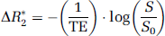
The numerical model was validated using phantom experiments by comparing a sagittal view of the transverse acquired magnitude images at different concentrations of contrast agent (0 to 15 mmol/L Gd-DTPA) and using the Pearson's correlation and RSS for quantitative validation (Figures 1 and 2). The images of the model show good agreement with the images of the phantom experiments. The acquisition voxel sizes of the simulation and phantom experiments are the same and similar to the voxel size of normal in vivo DSC-MRI protocols, although the pixel sizes in the images are different because of different shifting steps (0.5mm in both directions for the simulations, and 1.0mm (0.5mm for PRESTO) in the slice direction for the phantom experiments). It was concluded that the simulations provide a correct representation of the MR signal processes around a vessel during the passage of contrast agent.

Figure 1

Merged magnitude images (sagittal view) of the phantom experiments and the simulations for single-shot EPI (left), segmented EPI (TE₂; middle) and PRESTO (right) at three concentrations of Gd-DTPA (4.4, 8.8, and 13.2 mmol/L). The phantom images are formed by merging several multislice acquisitions (acquired in a transverse plane) that are shifted in the slice selection direction. Therefore, each pixel in this image represents a larger acquisition voxel. The phase encoding is oriented anterior to posterior. In the phantom, the stack of slices was shifted in steps of 1mm for both EPI acquisitions and in steps of 0.5mm for the PRESTO experiment. In the simulation, the stack of slices was shifted for all three acquisitions in steps of 0.5mm in the slice and phase encoding directions.

Figure 2

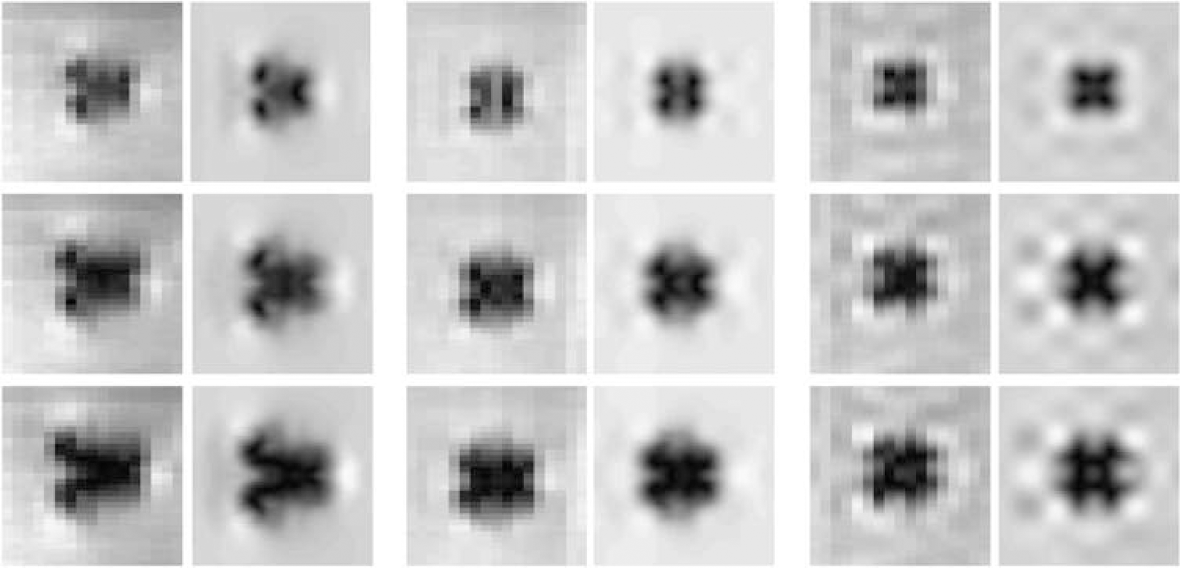
The relative signal strength (RSS in percent, first and third column) and correlation (second and fourth column) for the phantom experiments (first two columns) and the simulations (last two columns), with the MCA depicted as a white circle. From top to bottom: single-shot EPI, segmented EPI (TE₂) and PRESTO.

Advanced Model Evaluation

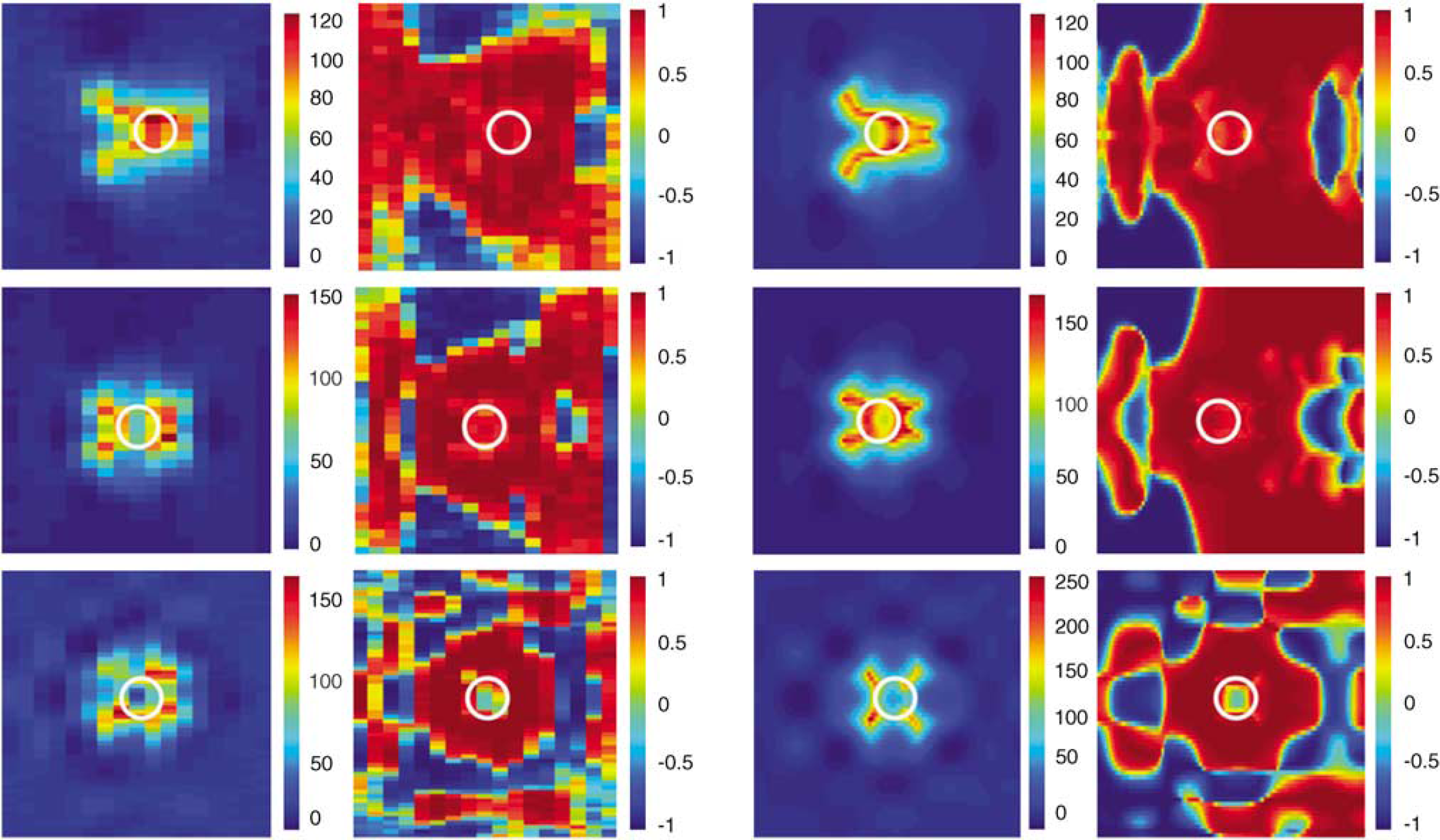
Figure 3 shows the normalized ΔR*₂ profiles of voxels acquired using segmented EPI (TE₂) in and around the MCA grouped according to the correlation about the ground truth. In the group with a correlation value between 0.7 and 0.8, peaks are observed on top of the passage curve that can be attributed to PVEs. In this study we define a correct measurement of the shape of the AIF as a correlation between the measured AIF and the ground truth that is higher than 0.99 (correlation values based on noise free simulations).

Figure 3

The measured AIF profiles of all simulated voxels for segmented EPI (TE₂) were normalized and grouped according to the correlation value with respect to the ground truth (between 0.7 and 0.8 (first graph), between 0.8 and 0.9 (second graph), between 0.9 and 0.95 (third graph), between 0.95 and 0.99 (fourth graph) and between 0.99 and 1 (fifth graph)). Upper row shows curves without tissue subtraction; lower row shows curves with tissue subtraction.

Figure 4 shows the results for PRESTO using in vessel strategy and both out vessel strategies. Independent of the used postprocessing strategy, the most optimal locations for AIF measurements were always observed outside the MCA. Optimal locations were found diagonally from the vessel center at a distance of approximately 4mm. Simulations were repeated, now with addition of Gaussian noise on top of the complex signals. This resulted in a lower correlation with the ground truth, whereas the signal strength remained unchanged.

Figure 4

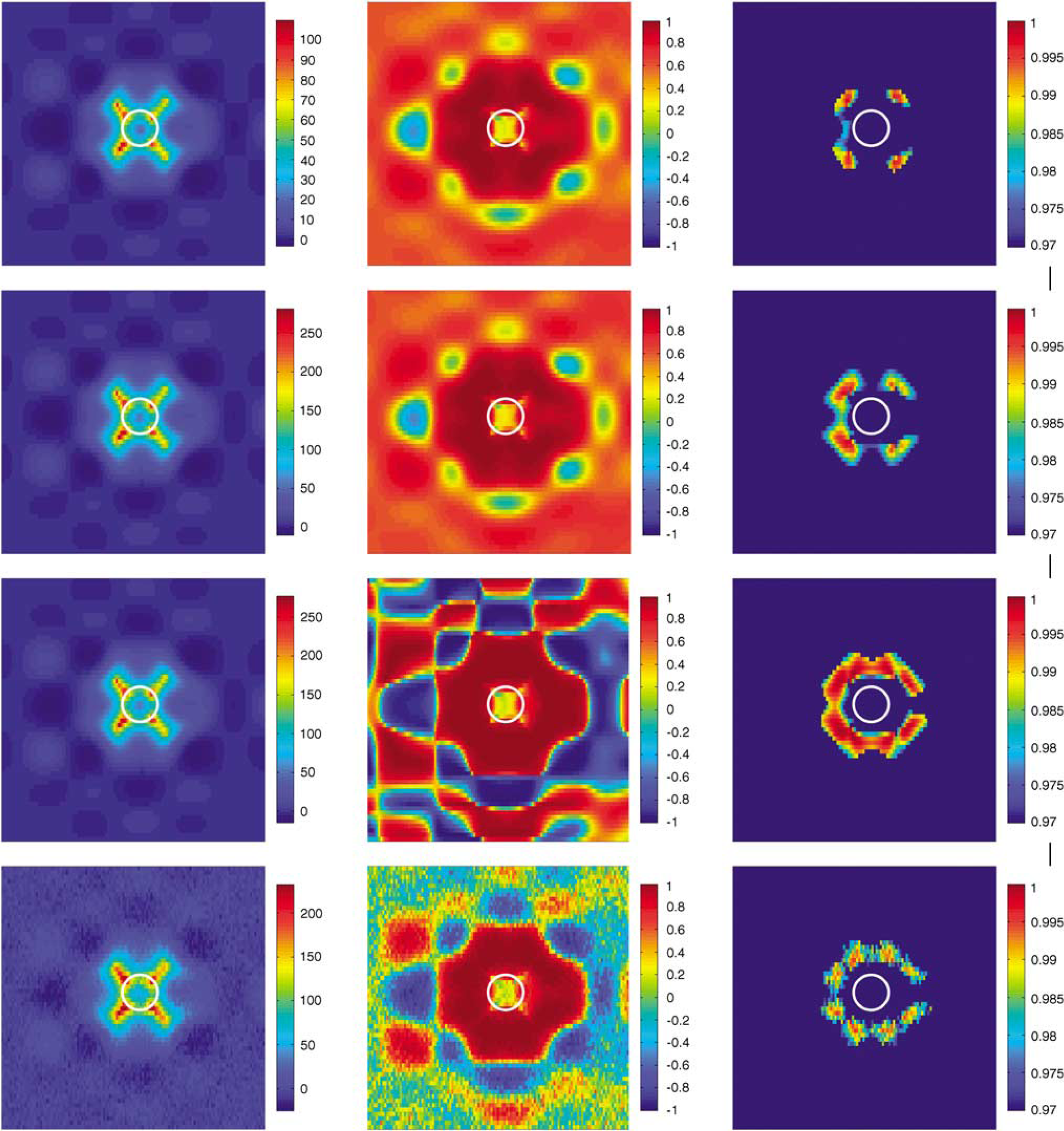
The relative signal strength (RSS in percent; left column), the correlation (middle column) and the RSS-thresholded correlation image (correlation coefficient larger than 0.97 and RSS larger than 25%; right column) for PRESTO at 1.5 T using the in vessel strategy (first row), out-vessel strategy (second row), out-vessel strategy with tissue subtraction (third row) and with noise included in the simulations (SNR=25 using out-vessel strategy with tissue curve subtraction; last row).

Three diameters of the MCA were investigated with the out-vessel strategy and tissue curve subtraction used for postprocessing (Figure 5). This resulted for single-shot EPI in some feasible locations for AIF determination, but not every position of the MCA within the imaging slice provided voxels that passed our criterion for correct shape measurement (correlation higher than 0.99 with the ground truth). For large and medium-sized vessels, the optimal location is found in an area 3.5 to 6mm posterior to the vessel center. Segmented EPI yields larger regions suitable for AIF selection. AIF selection using segmented EPI is less sensitive to the exact location of the vessel center within the imaging slice (Figure 5, second and third columns). Optimal locations are found all around the vessel (note that voxels located above the vessel are actually located in a slice superior to the slice through which the MCA runs). For the first echo time optimal locations are located relatively close to the vessel, but still outside the vessel, except for a small-sized MCA (Ø 2 mm), in this special case optimal locations are found within a circle approximately 4mm from the vessel center including voxels that are primarily sensitive to intravascular signal. For the longer echo time, optimal locations are found at a larger distance from the vessel center. Also for PRESTO, the optimal locations for AIF selection are found outside the vessel in the surrounding tissue, but here the optimal locations are found on the diagonal axes from the vessel center (Figure 5, fourth column).

Figure 5

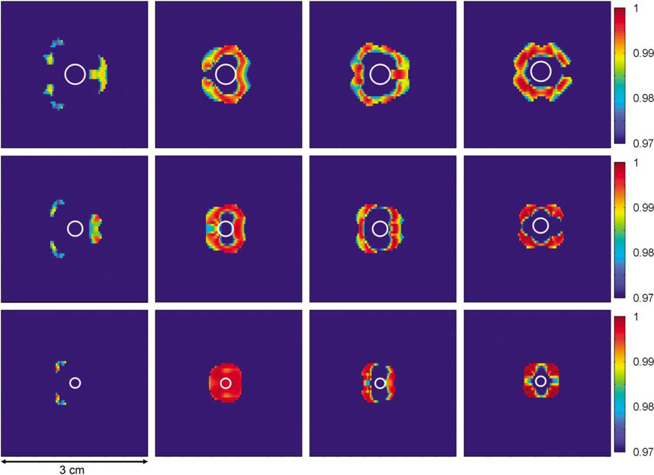
The RSS-thresholded correlation image (correlation coefficient larger than 0.97 and a voxel with greater than 25% RSS) for single-shot EPI (first column), segmented EPI (TE₁ and TE₂, second and third column, respectively) and PRESTO (fourth column) using the optimal strategy for measurements outside the vessel. Different rows represent different vessel sizes, diameters (respectively 4, 3, and 2 mm).

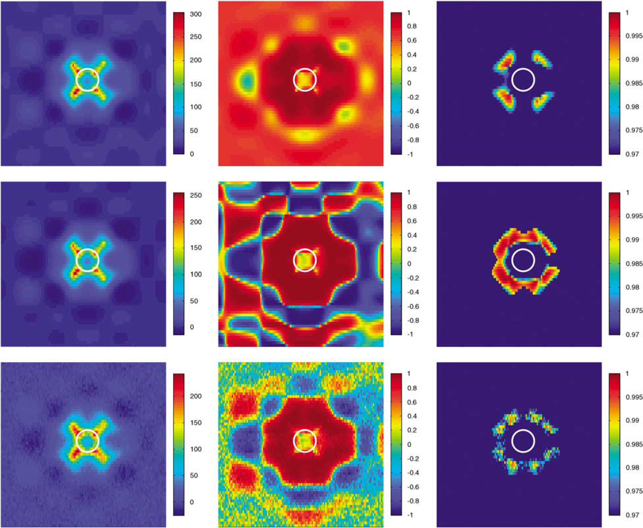
Figure 6 shows the results of the simulations performed using 3T literature values for PRESTO image formation. These results are comparable to the findings of the 1.5T simulations (compare to Figure 4).

Figure 6

The relative signal strength (RSS in percent; left column), the correlation (middle column) and the RSS-thresholded correlation image (correlation coefficient larger than 0.97 and RSS larger than 25%; right column) for PRESTO at 3.0 T using out-vessel strategy (first row), out-vessel strategy with tissue subtraction (second row) and with noise included in the simulations (SNR=25 using out-vessel strategy with tissue curve subtraction; last row).

In Vivo Example

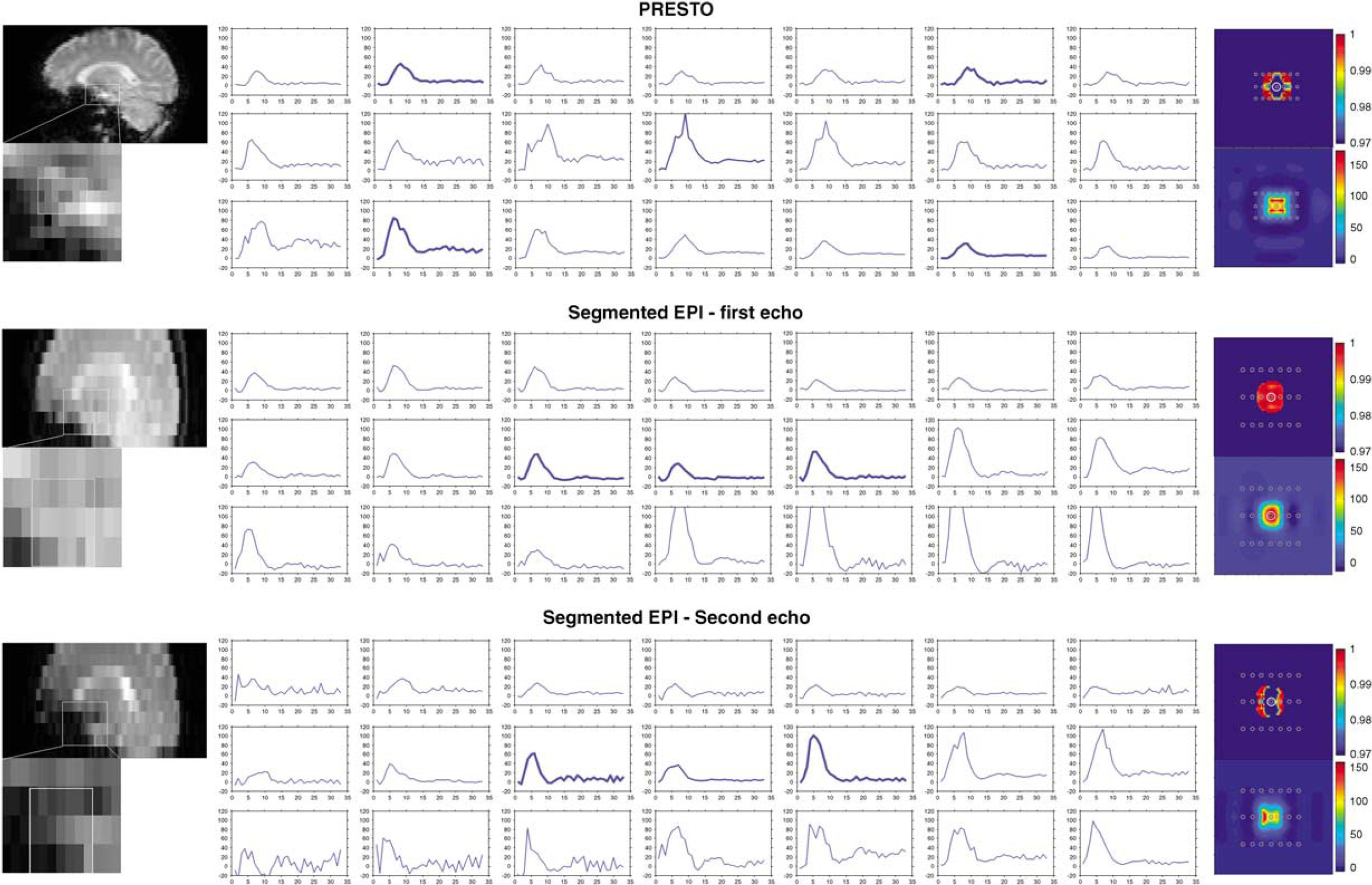
Figure 7 shows the ΔR*₂ bolus-passage measured in voxels closest to the MCA (middle profile is encompassing the vessel). The thickest lines are the optimal locations as predicted by simulations. Notice, that signs of PVEs, like peaks on the ΔR*₂ curves are almost absent in the selected curves. For the PRESTO sequence it is obvious that voxels in or directly anterior or posterior to the vessel, show most artifacts. Voxels located superior or inferior from the MCA show still reasonable signal strength without erroneous peaks, although the SNR is lower than for the voxels in and next to the MCA. The AIF measurements obtained from segmented EPI-TE₁ (middle panel) show for a large region in and around the MCA curves with little to no shape errors. This is in good agreement with the simulations. However, the signal strength of the curves is higher outside the MCA than predicted from the simulations. For segmented EPI-TE₂ (lower panel) the signal strength in the voxel encompassing the MCA is lower than the signal strength in the voxels located anterior or posterior from the MCA as expected from simulations. The shape in the voxels directly anterior or posterior from the MCA is also free of peaks or other signs of PVEs. This is also in agreement with the simulations.

Figure 7

In vivo example of AIF selection near the MCA. A straight part of the MCA angulated perpendicular to the main magnetic field was visually identified on the 3D T₁-weighted scan and this location was transferred to the DSC images; PRESTO (upper panel) and dual echo segmented EPI (middle and lower panel). ΔR*₂ curves were plotted for voxels located on and around the MCA; the ΔR*₂ curve of the voxel on top of the MCA was indicated with a thicker than normal line. On the basis of the findings in the simulation study, the curves from the optimal location for AIF measurements were plotted with the thickest lines. The corresponding simulation results are shown on the right side (thresholded correlation maps (upper) and relative signal strength (lower)), with the approximate location of the voxels indicated by gray circles.

Discussion

The main findings of this study are fourfold. First, AIF measurements near the MCA are best performed in voxels located completely outside the artery, within tissue surrounding the MCA. Second, a linear relation between ΔR*₂ and the concentration of Gd-DTPA is the best assumption when measuring the AIF in voxels that are not completely located inside the MCA. Third, the position with respect to the MCA that yields a correct AIF measurement depends on the particular imaging sequence, echo time and diameter of the MCA. Finally, AIF measurements can also be performed in voxels that encompass the MCA for a specific combination of small MCA and short echo time (TE₁) when using a segmented EPI readout.

In this study, we focused on finding the optimal location for AIF selection near the MCA based on theoretical modeling and evaluated this finding in an in vivo example. Using the MCA for AIF selection has several advantages: the MCA is almost always located inside the imaging volume, whereas AIF measurements in the ICA require the acquisition of an additional slice; second, the angle between the vessel axis and the main magnetic field is approximately 90°, resulting in maximal signal change in the surrounding tissue.

This study shows that AIF measurements are best performed in tissue near the MCA rather than in voxels that partly encompass the artery. This finding can be counterintuitive because in the brain, the contrast agent resides intravascular and therefore one may be tempted to assume that voxels within an artery provide the best opportunity for measuring the AIF. However, the presence of contrast agent within the MCA causes local magnetic field changes inside and outside the vessel and thus also affects the gradient echo MR signal outside the vessel. Furthermore, AIF measurements encompassing or partly in the MCA are hampered by PVEs. When the bolus contrast agent passes through the artery and alters the relaxivity, this leads to a smaller transverse relaxation rate for the intravascular compartment and the phase of this compartment will change because of altered susceptibility. The presence of contrast agent within the MCA will also lead to magnetic field changes in the surrounding tissue. Averaging over the extravascular compartment will therefore lead to dephasing and a general shift in phase of the signal will occur. When the total signal of partial volume voxels is formed, the contributions of the two compartments can add either constructively or destructively, depending on the relative phase difference between the two compartments. Destructive addition of the intra- and extravascular signal can lead to almost zero total signal resulting in a high value of ΔR*₂, showing as a sharp peak in the ΔR*₂ curves. Such peaks in the ΔR*₂ profiles can be observed in the simulation as well as in the in vivo AIF measurements (Figures 3 and 7). Figure 3 also shows that PVEs can lead to smaller widths or higher peaks in the ΔR*₂ profile, illustrating that AIF selection rules based on a small width or maximum height of the ΔR*₂ profile do not always exclude voxels that exhibit PVEs.

The effect of errors in shape of the measured AIF on CBF and the influence of the deconvolution technique has been studied by Calamante and Connelly (2007). It was concluded that the influence of erroneous AIF measurement on the CBF was highly dependent on the type of shape changes of the AIF, e.g. a too steep rise of the AIF resulted in the highest errors in CBF (Calamante and Connelly, 2007). The advanced model simulations show correct measurements of the AIF shape near the MCA as evidenced by high correlation values with the ground truth. It is difficult to translate these correlation values into expected errors in CBF measurements, since these will depend strongly on the used deconvolution technique (Ostergaard et al, 1996; Rempp et al, 1994; Vonken et al, 1999), especially as each deconvolution technique uses a different approach to suppress noise. To avoid the influence of a particular deconvolution technique on our results, it was chosen to use a quality parameter of the shape of the AIF instead. A correct shape of the AIF will yield correct relative CBF and CBV values, and correct absolute MTT values, because CBV and CBF scale equally with the amplitude of the AIF. When using an additional method for quantitative CBV measurements (e.g. Bookend Method; Sakaie et al, 2005) or quantitative CBF measurement (like arterial spin labeling; Williams et al, 1992) all perfusion measures can be quantified.

We used three different strategies for the conversion of MR signal changes to concentration of Gd-DTPA. In the first strategy a quadratic relation between ΔR*₂ and concentration of contrast agent was used, which is in correspondence with the relation as measured in human blood (van Osch et al, 2003a) (a strategy optimized for intravascular AIF measurements). The second strategy is optimized for AIF measurements in tissue in the direct vicinity of the artery. Traditionally, a linear relaxivity constant is used for AIF measurements outside the artery and this approach was therefore adopted for the second strategy. However, voxels located outside the MCA are not only subjected to signal changes caused by the presence of contrast agent within the MCA, but experience also signal changes because of the passage of contrast agent through the microvasculature of the tissue. Therefore a third strategy was used using a previously proposed method to reduce the effect of the tissue passage (Thornton et al, 2006). This approach is based on the subtraction of the ΔR*₂ curve of pure gray matter from the measured AIF. When our simulations were performed without noise, tissue subtraction resulted in almost complete elimination of the tissue passage curve from the measured AIF (Figure 3). However, for the simulations that included noise, tissue subtraction did not improve the shape and induced sometimes even undesired errors in shape. It can therefore be concluded that the out-vessel strategy without tissue curve subtraction provided the best opportunities for a correct AIF measurement, but an improved tissue subtraction approach does certainly provide opportunities for even better AIF measurements. The simulations also showed that a linear relation between ΔR*₂ and concentration contrast agent is the best assumption when converting MR signal changes into concentration time curves for AIF measurements outside the MCA.

The exact location for optimal AIF measurement in the tissue surrounding the MCA differs for the various sequences that were studied. Voxels for AIF measurements using PRESTO should be selected above or beneath the vessel and posterior or anterior to the vessel. For single-shot EPI, the optimal location is found in tissue posterior to the vessel. For certain positions of the vessel center within the imaging slices none of the voxels fulfilled our criteria when using single-shot EPI. Segmented EPI showed more feasible locations for AIF measurements. For the second echo time, correct locations are found both anterior and posterior to the vessel, and are in some cases found in the slice superior or inferior to the MCA. When using the first echo time the best locations are found closer to the vessel. For a relatively small MCA (Ø 2 mm), short-echo-segmented EPI also gives correct AIF measurements for voxels partly in the MCA.

Imaging using longer echo times causes larger signal drops both inside and outside the vessel. For these longer echo times, the intravascular signal drops into the noise level for relatively small concentrations of contrast agent. The relative contribution of the intra- versus extra-vascular compartments will therefore change significantly when measuring the AIF in voxels encompassing the MCA, leading to an erroneous shape. However, also the extravascular signal will at some point drop into the noise-level, at which point noise will dominate the ΔR*₂ measurement, thereby affecting the shape of the curve, especially the peak, dramatically. Therefore not only PVEs but also signal saturation and noise can lead to errors in the measured shape of the AIF. The influence of the echo time on the occurrence of signal saturation can be observed in the results of the dual echo segmented EPI (Figure 5), which show optimal locations for AIF measurement much closer or even on top of the MCA for the shorter echo time compared with the longer echo time. This can be explained by the fact that the extent of the field inhomogeneities increase with longer echo times, leading to signal saturation at larger distances from the vessel center. The finding of correct AIF measurements, using segmented EPI with a short echo time, on top of the MCA could be useful for local AIF selection methods, where AIF measurements are performed at the level of small arteries that supply the adjacent tissue with blood. However, further research is required to determine the effect of the orientation and the exact size of the small artery on the shape of the AIF measurements.

The findings from the simulations were subsequently applied to an in vivo example (Figure 7). Although in general the findings of the simulations were reproduced in this in vivo example, some discrepancies were observed. In our opinion, these differences can be explained by uncertainties in the exact location of the MCA in the DSC images, as movement of the patient and distortions of the MR images can lead to misidentification of the location of the MCA. However, several important observations can be made from this example. First, the short echo time of the segmented EPI sequence, did indeed lead to a large region around the MCA where the AIF can be measured without suffering from PVEs, like erroneous peaks on the AIF. When comparing the short echo time data with the second echo time, it is clear that the number of voxels showing correct AIF shape is much lower when using the longer echo time. Second, the PRESTO data (upper panel) show that AIF measurements can indeed better performed in the slice above or below the MCA, as voxels in these curves show less erroneous deformations than the voxels located in the same slice as the MCA. Furthermore, it is clear that the SNR of a single voxel is too low when using it as input for the deconvolution analysis. In general, the SNR of the AIF can be improved by averaging a number of AIF measurements with correct shape, e.g. along the MCA or in voxels around the MCA (when using segmented EPI with a short echo time). However, care should be taken to avoid voxels where smaller arteries branch off the MCA.

All phantom experiments performed on 1.5 T resemble a concentration dose of 0.2 mmol/kg-bodyweight Gd-DTPA. The in vivo experiments performed at 3 T used 0.1 mmol/kg-bodyweight Gd-DTPA. The susceptibility changes, field strength, and echo train length have the largest contribution to the pattern of signal decreases observed in and outside the vessel for gradient echo images. With double the field strength and half the concentration Gd-DTPA the signal decrease patterns will remain comparable, as both effects cancel out, although other differences (e.g. resulting from differences in relaxation rates and values) might lead to discrepancies. Nonetheless, when repeating the simulations for 3.0 T with half the dose of contrast agent, the same optimal locations were found as observed in the simulations of 1.5 T (compare Figures 4 and 6).

The advanced numerical model was designed to closely resemble in vivo AIF selection in or near the MCA, still some assumptions had to be made. First, the MCA was modeled as an infinite cylinder oriented perpendicular to the main magnetic field; therefore the conclusions only holds for a straight part of the MCA at least four times the diameter (Bhagwandien et al, 1994). The cardiac effects on the MCA were not taken into account. Imaging with single-shot EPI takes on the order of 0.1 sec and can be considered as a snapshot compared with the cardiac cycle (approximately 0.8 sec). PRESTO was used as a 3D sequence and takes approximately 2 cardiac cycles (1.5 or 2 secs), however the large gradients used for echo-shifting crush the intravascular signal.

In summary, AIF measurements are best performed using a short echo time in combination with segmented EPI. For this setup a large area around the MCA provide AIF curves with little errors because of PVEs and signal depletion, leading to the best measurement of the shape of the AIF. In most situations, the AIF measurement is best performed in voxels located completely in tissue surrounding the MCA. Segmented readout sequences such as segmented EPI or PRESTO result in more possible locations for AIF selection and are less sensitive to the exact position of the vessel in the through-plane direction than single-shot EPI. For most sequences, the best location for AIF measurements is posterior to the vessel and is for some cases found in the slice superior to the MCA. Converting the MR signal to concentration of contrast agent is best performed using a linear relation when measuring outside the artery.