Validating a Local Arterial Input Function Method for Improved Perfusion Quantification in Stroke

Abstract

In bolus-tracking perfusion magnetic resonance imaging (MRI), temporal dispersion of the contrast bolus due to stenosis or collateral supply presents a significant problem for accurate perfusion quantification in stroke. One means to reduce the associated perfusion errors is to deconvolve the bolus concentration time-course data with local Arterial Input Functions (AIFs) measured close to the capillary bed and downstream of the arterial abnormalities causing dispersion. Because the MRI voxel resolution precludes direct local AIF measurements, they must be extrapolated from the surrounding data. To date, there have been no published studies directly validating these local AIFs. We assess the effectiveness of local AIFs in reducing dispersion-induced perfusion error by measuring the residual dispersion remaining in the local AIF deconvolved perfusion maps. Two approaches to locating the local AIF voxels are assessed and compared with a global AIF deconvolution across 19 bolus-tracking data sets from patients with stroke. The local AIF methods reduced dispersion in the majority of data sets, suggesting more accurate perfusion quantification. Importantly, the validation inherently identifies potential areas for perfusion underestimation. This is valuable information for the identification of at-risk tissue and management of stroke patients.

Introduction

Bolus-tracking magnetic resonance imaging (MRI) is frequently used to quantify perfusion in stroke patients via an intravenous injection of paramagnetic contrast followed by repeated acquisition of magnetic resonance images to track the bolus passage through the brain (Ostergaard et al, 1996a, 1996b). Commonly, a global Arterial Input Function (AIF) is measured by averaging the bolus concentration time-course (CTC) profiles in voxels selected near a major contralateral artery (Calamante et al, 1999). Perfusion maps are calculated by deconvolving this AIF from whole brain CTC data (Ostergaard et al, 1996b). In stroke patients, delay and temporal dispersion (D/D) of the bolus may be considerable in the ipsilateral hemisphere (IH) due to arterial stenosis, occlusions, or collateral flow (Calamante et al, 2003). Since D/D is not included in the measured global AIF (GAIF), the severity and extent of any perfusion deficit may be exaggerated (Calamante et al, 2000). Such misdiagnosis may lead to dangerous mistreatment, since tissues that are not at risk of infarction may appear to be so due to erroneously low perfusion estimates resulting from the D/D.

Although deconvolution algorithms can be made delay-insensitive, e.g., singular value decomposition with a block-circulant deconvolution matrix (oSVD) (Wu et al, 2003), dispersion cannot be easily accounted for in standard deconvolution methods. Dispersion error may be circumvented using multiple local AIFs—located downstream of any arterial abnormality—to deconvolve small branch arterial territories. Previously suggested methods to identify the local AIFs include: automated heuristic approaches to select CTC profiles appearing most arterial (Alsop et al, 2002; Lorenz et al, 2006b); and spatial Independent Component Analysis of the CTC map to isolate the arterial-like temporal components (Calamante et al, 2004). These methods assumed that a region of tissue is fed mainly by the local AIF to which it is spatially closest. However, near vascular territory boundaries this assumption may not hold. In the present work, we assign arterial territories based on spatial closeness and temporal similarities (specifically, similar bolus arrival times (BATs)) between the local AIF and tissue CTC.

Although some studies have investigated the potential role of local AIFs in predicting stroke outcome (Christensen et al, 2009; Lorenz et al, 2006a), to date there are no published studies investigating the veracity of the estimated local AIFs. The validity of the local AIFs can be indirectly inferred through the minimization of D/D, since reduced D/D indicates a more accurate AIF, and consequently, a more accurate perfusion estimate. Here, we evaluate two local AIF methods (including one novel method that is introduced in this work), and compare them with the standard GAIF analysis by measuring the dispersion remaining after deconvolution.

Materials and methods

Local Arterial Input Function

In this study, the principles for identifying local AIFs and their territories were based on those presented by Christensen et al (2008), as follows: along the supply route and toward the distal small branches of the arterial tree, blood arrives later (increasing BAT) and flows more slowly (increasing intervoxel BAT differences). At typical temporal resolution repetition time (TR) (1.5 to 2.5 seconds), only the larger local BAT differences in the smaller distal arteries are detectable: the relatively low flow speeds of small pial arteries translate to a BAT difference of ∼150 ms between voxels spaced 2 mm apart; in contrast, at the higher velocities in large arteries this time difference would be only a few milliseconds, too small to be detected with the TRs of bolus-tracking MRI (see Christensen et al (2008) for more detail on this argument). Therefore, the small branch vascular territory is determined by following the lowest BAT gradient descent path from each tissue voxel toward a local minimum, inferred as the local origin of supply, i.e., the local AIF voxel. This approach assumes that voxels supplied by the same local AIF have similar BATs, and that the supply route has no large BAT discontinuities. Voxels belonging to the same local AIF territory are therefore both spatially close and temporally similar.

Given that the in vivo data used in this study was a 2D acquisition (see later for more detail on the bolus-tracking protocol), with relatively thick slices (6 mm) and a large interslice gap (7 mm) compared with a 1.56 × 1.56 mm in plane resolution, the local minima were found by scanning a 2D within-slice 3 × 3 voxel neighborhood. Performing a 3D search for the local minimum would introduce significant bias toward finding through-slice major arteries, thus resulting in main territory AIFs. Rather, we are interested in finding local AIF territories so as to minimize delay and dispersion. The within-slice 2D search also avoids slice-timing complications and anisotropic 3D voxel bias. It should be noted that the 2D search of local minima should avoid large BAT discontinuities and therefore, even if the local feeding artery is in a different slice, the algorithm is expected to find the local minima as the entrance of that artery to the slice or as a nearby small artery with similar bolus shape. However, if more isotropic voxels are available, the search should be performed within a 3 × 3 × 3 voxel neighborhood.

In practice, the small BAT differences, ΔBAT, were measured by first fitting gamma-variate (GV) functions (Harpen and Lecklitner, 1984) to all the CTCs. Due to irregular and bumpy CTCs arising from noise, motion, and various scanning artifacts (e.g., partial volume and susceptibility-related shifted voxels), it can be difficult to fit accurately a GV function. Therefore, the most rough and erratic CTCs (and hence poor local AIF estimates) were discarded before GV fitting to minimize the risk of erroneous BAT estimates. The excluded CTCs were identified by one or more of the following properties in a numerical calculation: negative cerebral blood volume; ratio of negative to positive area under CTC >0.5; contrast-to-noise ratio, (defined as peak of first passage to prebolus baseline standard deviation) <1; time-to-peak of CTC >25 seconds after median time-to-peak for that slice; or First Moment (FM) less than upslope of first passage. For the remaining CTCs, GV fitting was implemented using the Simplex algorithm.

In this work, the BAT was estimated using two different approximations. First, BAT was estimated as the FM of the GV fitted CTC, FM_C, which was shown by Christensen et al (2008) to be more robust than estimating BAT directly from the parameter of the GV fitting. The method of identifying local AIF sources and territories from an FM_C map (Christensen et al, 2007) will from herein be referred to as LAIF1.

Although FM_C was used previously to identify local AIF sources, (Christensen et al, 2007, 2008), its mean transit time (MTT) dependence may be problematic for locating local AIFs in transition regions between normal and abnormally perfused tissue. Hypoperfused tissue has a prolonged MTT and broader tissue CTC, causing correspondingly larger FM_C. In this situation, FM_C is biased toward finding BAT minima outside of the hypoperfused area, possibly resulting in an inappropriate local AIF, leading to errors in estimating the area of abnormal perfusion and thus the diffusion-perfusion mismatch. We propose estimating BAT using an adjusted parameter, FM_adj which is specifically designed to have low sensitivity to MTT variations (see Appendix):

$$F{M}_{\mathrm{a}\mathrm{d}\mathrm{j}}=F{M}_{\mathrm{C}}-F{M}_{\mathrm{R}}+Tmax$$

(1)

where FM_R is the FM of the tissue residue function calculated using a GAIF oSVD deconvolution, and Tmax is the time-to-peak of that same residue function. This new method of identifying local AIF sources and territories from an FM_adj map will from herein be referred to as LAIF2.

Following the identification of potential local AIF voxels and their associated territories using either LAIF1 or LAIF2, heuristic criteria similar to those in Mouridsen et al (2006) were applied to disregard the 10% of local AIFs with smallest area, and the 10% with largest roughness. Tissue voxels linked to an invalid local AIF were assigned the local AIF of the nearest neighboring territory. Finally, all local AIF curves were normalized to unit area. Automated methodologies for selecting the local AIFs of LAIF1 and LAIF2 were implemented in MATLAB (Mathworks, Natick, MA, USA).

Simulated Data

To demonstrate the limitations of the LAIF1 method and investigate the approximations involved in the design of the LAIF2 method, the dependence of their respective BAT estimates, FM_C and FM_adj, on delay, dispersion, and MTT, were studied using a simulated bolus-tracking data set, described previously in Willats et al (2006). The microvascular retention parameters were cerebral blood volume=4% and MTT=3 to 12 seconds (1 second steps); the macrovascular transport parameters were delay=0 to 5 seconds (0.5 second steps) and dispersion=0 to 6 seconds (1 second steps), where dispersion is defined as the FM of an exponential Vascular Transport Function (Calamante et al, 2000); signal-to-noise ratio=33, 50, and 100, defined from the prebolus baseline magnetic resonance signal (S_prebolus/σ(S_prebolus)); TR=1 to 2.5 seconds (0.5 second steps). The AIF was modelled as a GV function with recirculation, as described in Ostergaard et al (1996b). For each microvascular/macrovascular/noise/TR parameter combination (9,240 total) the mean and standard deviations of FM_C and FM_adj were measured from 100 data sets generated with random additive Gaussian noise corresponding to the signal-to-noise ratio.

In Vivo Data and Analysis

Nineteen bolus-tracking MRI data sets from 17 patients were retrospectively selected from clinical scans acquired between 2001 and 2006 from anterior circulation stroke patients. Consent was obtained from all participants and the study protocol was approved by the local (Austin Health) Ethics Committee. The selection criteria were minimal patient motion during the bolus passage, and an MTT abnormality based on conventional analysis of bolus-tracking data. For the purpose of this study, conventional analysis corresponded to using the delay-insensitive oSVD deconvolution with a GAIF automatically measured in a branch of the contralateral middle cerebral artery. This analysis was carried out using the PENGUIN software (PErfusioN Graphical User INterface; http://www.cfin.au.dk/software/penguin), and provided a preliminary indication of the perfusion abnormality, though possibly exaggerated by dispersion (but not delay). For all the analyses (local and global AIF methodologies), the CTC data were calculated assuming a linear relationship between the transverse relaxation rate change and contrast concentration (Calamante et al, 1999). The perfusion MRI data were acquired on a 1.5 T General Electric Signa Horizontal SR 120 (General Electric, Milwaukee, WI, USA) using a gradient-echo echo planar imaging and 0.2 mmol/kg bolus of a Gd-based contrast agent injected by a power injector and followed by 15 mL saline. The sequence parameters were echo time/TR=60/1,740 ms and 10 slices, echo time/TR=70/2,240 ms and 12 slices, or echo time/TR=60/1,999 ms and 12 slices; 256 × 256 matrix; slice thickness=6 mm; slice spacing=7 mm; voxel size 1.56 × 1.56 mm. For the corresponding diffusion images, echo time/TR=100/12,000 ms, 19 slices, 256 × 256 matrix, slice thickness=5 mm, slice spacing=6.7 mm, voxel size 1.56 × 1.56 mm, and b value 1,000 s/mm².

FM_C and FM_adj maps were calculated and the LAIF1 and LAIF2 local AIF voxels were identified as the respective local minima with perfusion territories determined as described previously. Perfusion maps were estimated from the maximum of the Fourier-interpolated (Salluzzi et al, 2006) tissue response functions (Ostergaard et al, 1996a), calculated by oSVD deconvolution (Wu et al, 2003) of the local AIFs. Cerebral blood volume maps were estimated by integrating the first pass of the CTCs, and relative MTT maps were calculated using the Central Volume Theorem (Calamante et al, 1999). The process for obtaining the MTT maps from GAIF, LAIF1, and LAIF2 oSVD deconvolution is summarized in section (a) of the flow chart in Figure 1.

Figure 1

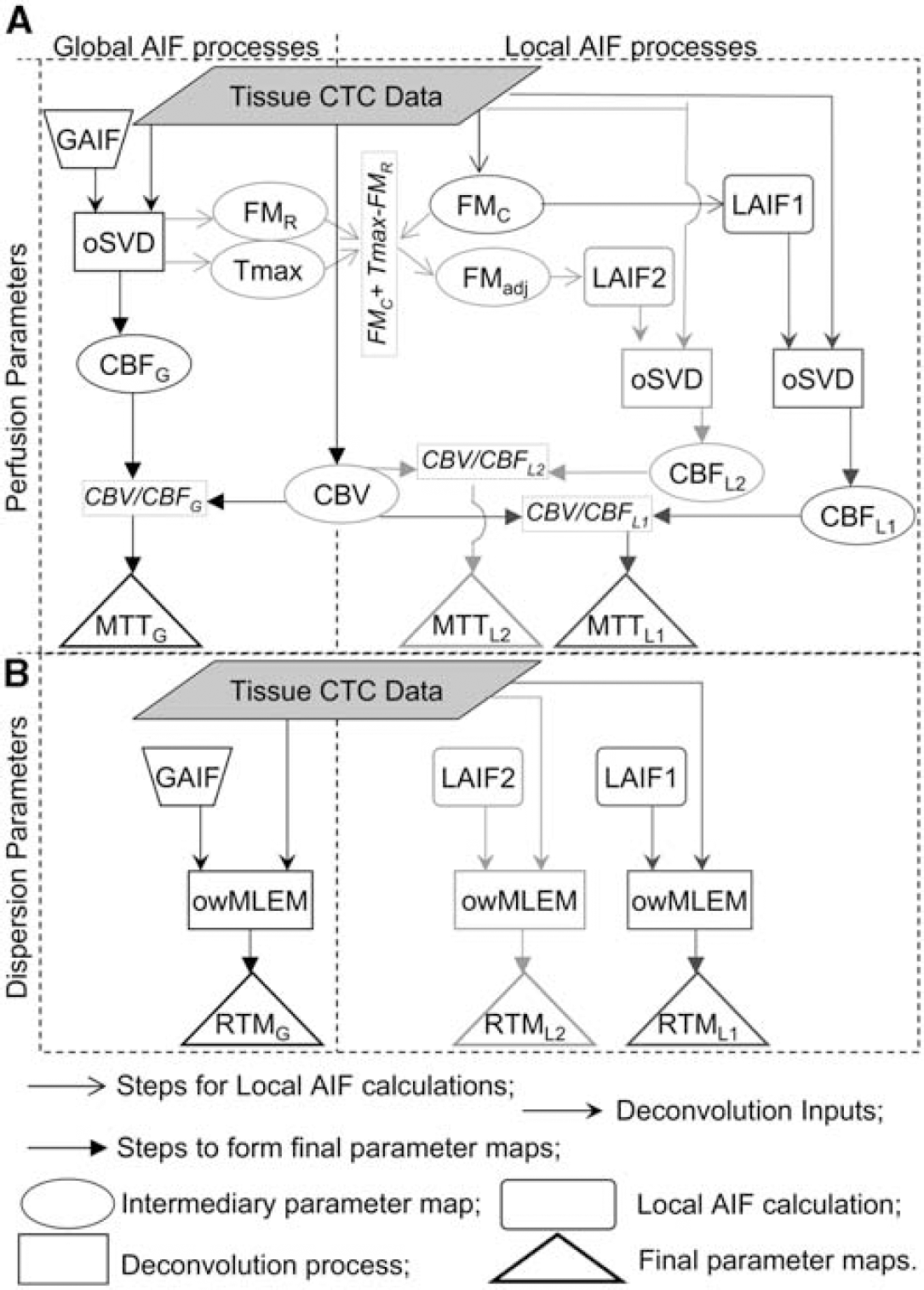
Flow chart outlining the steps involved in forming the various parameter maps, and their relationship to each other. The chart is divided into four quadrants. The top two quadrants (A) contain processes for calculating perfusion maps using global AIF (GAIF, left) and local AIFs (LAIF1 and LAIF2, right). The bottom two quadrants (B) show the process for obtaining the dispersion maps from GAIF (left) and from LAIF1 and LAIF2 (right). Note that in (B) the Tissue CTC Data, GAIF, LAIF1, and LAIF2 are taken from section (A). The subscripts G, L1, and L2 refer to the maps obtained using GAIF, LAIF1, and LAIF2, respectively. For further clarity, the GAIF steps are in black, the LAIF1 steps are in blue, and the LAIF2 steps are in red. AIF, Arterial Input Function; CTC, concentration time-course; GAIF, global AIF; oSVD, delay-insensitive deconvolution; Tmax, time-to-maximum value of GAIF oSVD residue function; FM_R, First Moment of GAIF residue function; CBF, cerebral blood flow; MTT, mean transit time; CBV, cerebral blood volume; FM_adj, adjusted First Moment (equation (1)); FM_C, FM of the CTC; LAIF, local Arterial Input Function; owMLEM, maximum-likelihood expectation-maximization deconvolution regularized with an oscillation index and wavelet thresholding; RTM, time to rise-to-maximum value the owMLEM residue function.

A reference MTT value was estimated for each method (GAIF, LAIF1, and LAIF2) in each data set by manually segmenting the contralateral grey matter (GM) and averaging the MTT values, MTT_contraGM. Abnormal MTT areas were defined by highlighting ipsilateral voxels with MTT>Thld, where Thld=MTT_contraGM+1.78 seconds (Christensen et al, 2009). This threshold was shown in Christensen et al (2009) to have the greatest sensitivity and specificity for predicting future infarction from oSVD MTT maps. From herein, MTT above this threshold is referred to as abnormally (abn) perfused, or hypoperfused, and the hypoperfusion maps for GAIF, LAIF1, and LAIF2 are labelled as abnMTT_GAIF, abnMTT_LAIF1, and abnMTT_LAIF2, respectively. These are in fact apparent (rather than true) hypoperfusion maps since their MTT values may be biased by dispersion.

In the absence of delay and dispersion, the initial value of the tissue response functions, r(t), will also be its maximum. Where there is delay, this maximum is simply time shifted, and the shape of r(t) is maintained. However, where there is dispersion, the shape of r(t) becomes broader and flatter, resulting in a later and lower maximum value. Therefore, in theory it is possible to identify areas of dispersion-related erroneous perfusion from the shape of r(t) (Willats et al, 2008). However, due to the regularization effects in oSVD deconvolution, it is impossible to distinguish delay from dispersion in the shape of r_oSVD(t) (where r_oSVD(t) is the r(t) calculated using oSVD). In contrast, the ‘Maximum-Likelihood Expectation-Maximization deconvolution regularized with an oscillation index and wavelet-thresholding’ (owMLEM) method has been shown to characterize the tissue response more accurately (Willats et al, 2008), in particular the short sharp rise to maximum of a delayed r(t) is easily distinguished from the broader dispersed r(t). Therefore, delay may be estimated from the length of the r_MLEM(t) baseline and dispersion from the time to rise from baseline to maximum (rise-to-max or RTM) of r_MLEM(t). Given the limited temporal resolution, we distinguish dispersion as follows: RTM≥TR is dispersed; 0<RTM<TR is classified as not dispersed (N.B. it may include small sub-TR delay/dispersion, see Discussion). Fourier interpolation of r_MLEM(t) serves to minimize discretization errors in RTM. This measure of residual dispersion (i.e., RTM) indicates the accuracy of the corresponding MTT and therefore the validity of the associated AIF. For the in vivo data sets, RTM will be very small in regions where the AIF has successfully removed dispersion. For completeness, a diagrammatic representation of the validation steps to obtain the owMLEM RTM maps (from the GAIF, LAIF1, and LAIF2 analyses) is shown in section (b) of the flow chart in Figure 1.

Dispersion maps for GAIF, LAIF1, and LAIF2 were created by highlighting ‘abnormal’ voxels with RTM≥TR (maps labelled abnRTM_GAIF, abnRTM_LAIF1 and abnRTM_LAIF2, respectively). These maps indicate areas affected by residual vascular dispersion, where the MTT estimates are thought to be unreliable (Willats et al, 2008).

The sizes of the highlighted (abnormal) regions in the abnMTT and abnRTM maps described above were expressed as a percentage of the IH excluding ventricles (%abnMTT and %abnRTM, respectively), for a single slice with significant diffusion abnormality. The sizes of these abnormal regions were pairwise compared between each method (GAIF versus LAIF1, GAIF versus LAIF2, and LAIF1 versus LAIF2). Comparisons were done using a signed Wilcoxon's test. To aid discussion, the data sets were ordered according to the difference in dispersion area between %abnRTM_GAIF and %abnRTM_LAIF2, and labelled from A to S accordingly. A summary of information for each data set is given in Table 1.

Table 1

Summary information for data sets A–S

Data set ID	Patient age (years)	Time of MR from stroke onset	MRA info and notes	Later DWI
A	72	53.6 hours	Same patient as data set H	None
B	76	6.17 hours	Patent	260 days
C	63	101 days	20–30% CCA occlusion in acute/patent in subacute	None
D	63	85 days	Occluded right ICA	None
E	78	4.1 hours	Patent	None
F	72	72 days	Patent	None
G	83	17.5 hours	No data	None
H	72	3.17 hours	Occlusion	53.6 hours
I	75	12.3 hours	Patent	None
J	70	24 hours	Patent	None
K	72	56 hours	Patent	None
L	45	36 hours	Patent	None
M	31	4 days	Patent	None
N	74	9.6 hours	Occluded left MCA	None
O	79	3 hours	Occluded left CCA ICA	108 days
P	35	32 hours	Same patient as data set S	93 days
Q	65	12 hours	Occlusion	None
R	53	48 hours	Patent	None
S	35	8.45 hours	ICA dissection	93 days

MRA, magnetic resonance angiography; CCA, common carotid artery; ICA, internal carotid artery; MCA, middle cerebral artery; DWI, diffusion weighted imaging. The underlined letters correspond to the results illustrated in Figure 4. None of the patients received thrombolytic treatment.

Results

Simulated Data

Figure 2 shows the dependence of FM_C and FM_adj on delay, dispersion, and MTT for data simulated across typical parameters. FM_C has the desired (approximately proportional) dependence on delay and dispersion, but as predicted, is also (undesirably) strongly dependent on MTT. FM_adj also increases with delay and dispersion, but is much less influenced by MTT. We note that there is also some loss in precision, resulting from the addition of variance across the three combined variables in equation (A7) (Appendix). Results from other simulation parameters were qualitatively similar (data not shown).

Figure 2

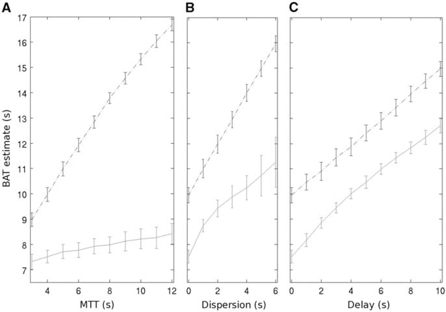
Example simulation results at TR=2 seconds and signal-to-noise ratio=50 showing the BAT estimate (FM_C=blue dashed-dot line, FM_adj=red solid line) as a function of (A) simulated MTT (delay=0 second, dispersion=0 second), (B) simulated dispersion (MTT=4 seconds, delay=0 second), and (C) simulated delay (MTT=4 seconds, dispersion=0 second). Error bars are ±1s.d. BAT, bolus arrival time; FM_C, First Moment of the concentration time-course, FM_adj, adjusted First Moment (equation (1)); MTT, mean transit time; TR, repetition time.

In theory, FM_adj should have reduced MTT dependence compared with FM_C, and Figure 2 suggests that this is indeed the case in practice, giving support to the approximations involved in the design of the LAIF2 method.

In Vivo Data

While there was an overall good agreement between the results using LAIF1 and LAIF2, LAIF2 was marginally better in reducing dispersion in all but one data set (data set C, where the %abnRTM_LAIF2 (=82%) was ∼4%IH larger than abnRTM_LAIF1 (=78%), data not shown). Accordingly, %abnRTM_LAIF2 was significantly smaller than %abnRTM_LAIF1 (P<0.001) in the paired comparison across all data sets. The following results will therefore focus on a comparison between GAIF and LAIF2.

Figure 3 indicates the size of the abnormal dispersion and apparent abnormal perfusion areas using GAIF and LAIF2. In all the data sets except A, B, and C, LAIF2 reduces the size of the dispersion area (%abnRTM_LAIF2<%abnRTM_GAIF), suggesting that the correspondingly smaller apparent hypoperfusion areas (%abnMTT_LAIF2<%abnMTT_GAIF) are less affected by dispersion error and therefore more likely to represent the true extent of the hypoperfusion. In data sets A, B, and C, LAIF2 slightly increased the dispersion area (∼10%IH). Closer inspection of the RTM images shows that the additional dispersion occurs primarily in areas of deep white matter where it is difficult to find a local AIF (e.g., data set A, Figure 4i). While this increase is not desirable, there is no corresponding increase in the area of apparent hypoperfusion in data sets A and B (%abnMTT_LAIF2≈%abnMTT_GAIF), indicating that any errors introduced by the additional dispersion are too small to recategorize this tissue as hypoperfused. In the remaining 16 data sets, LAIF2 reduces both the dispersion and apparent hypoperfusion areas to various extents as indicated in Figure 3. In the paired comparison across all data sets, %abnRTM_LAIF2 and %abnMTT_LAIF2 were significantly smaller than %abnRTM_GAIF and %abnMTT_GAIF, respectively (P<0.001).

Figure 3

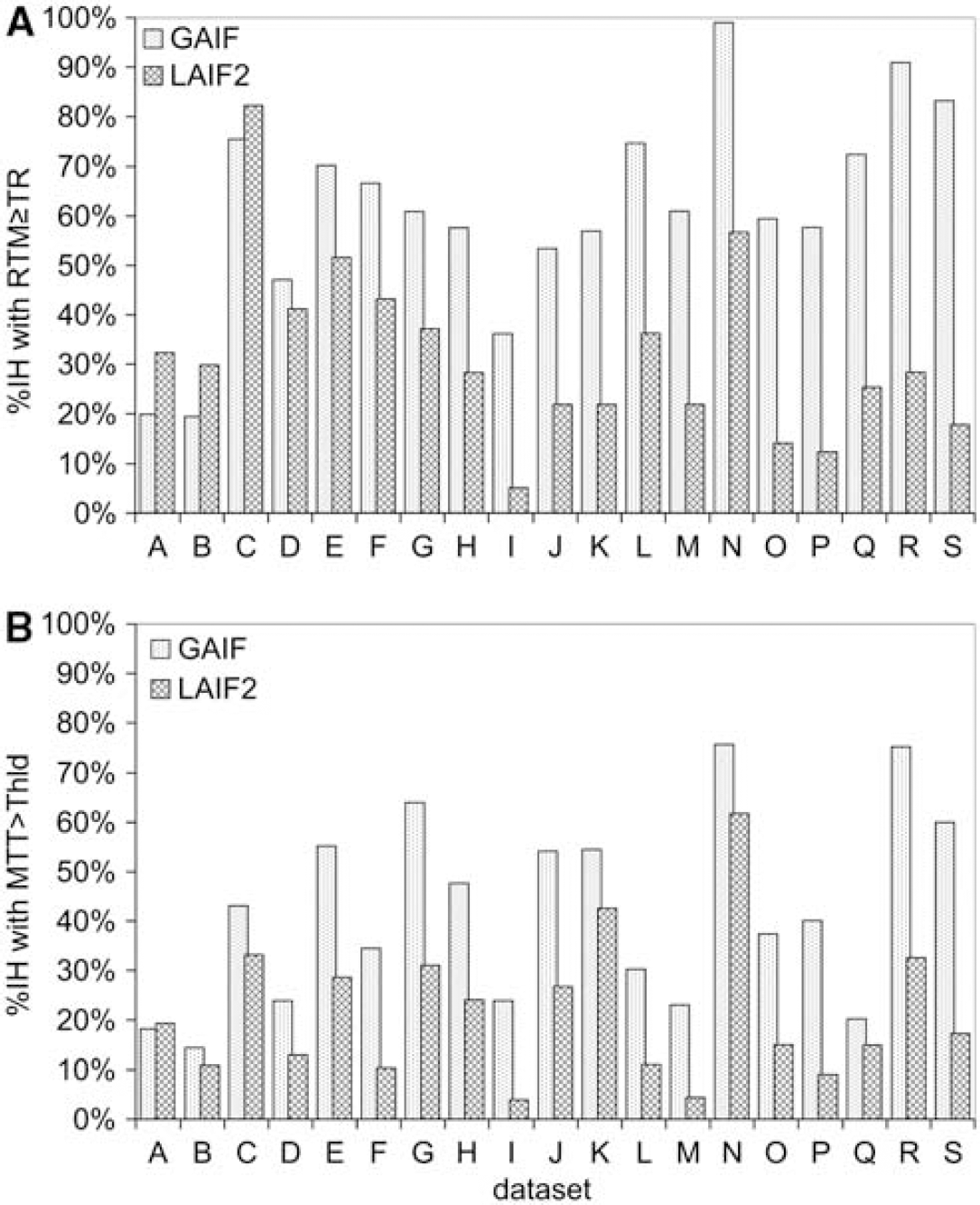
Graph showing the %IH with abnormality using GAIF (dotted bars) and LAIF2 (hashed bars). The top graph (A) shows the dispersion (RTM≥TR) and the bottom graph (B) shows the hypoperfusion (MTT>Thld) for each data set A–S. GAIF, global Arterial Input Function; LAIF2, local Arterial Input Function (new method); RTM, time to rise-to-maximum value of the owMLEM residue function; MTT, mean transit time; Thld=MTT_contraGM+1.78 seconds (see text); TR, repetition time.

Figure 4

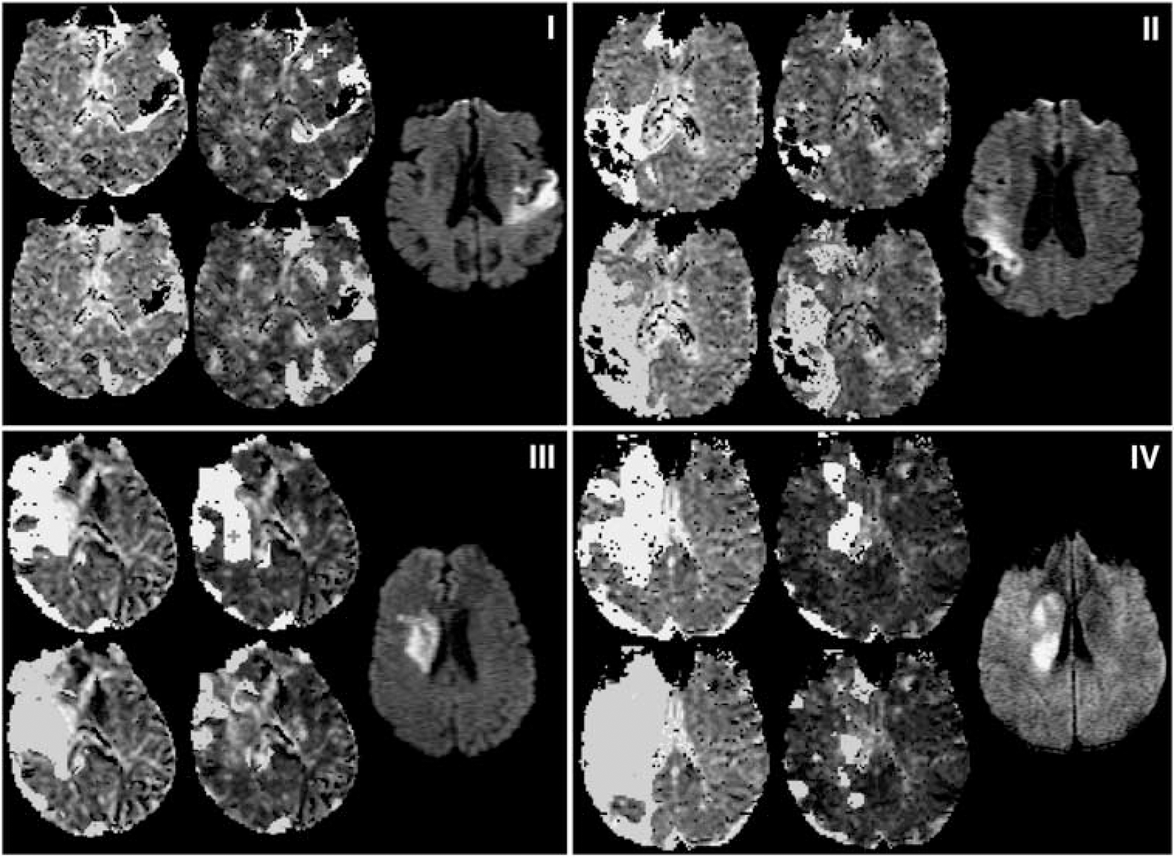
Abnormal perfusion and dispersion areas from example slices in data sets A (i), F (ii), K (iii), and S (iv). In each subfigure (i–iv), the diffusion weighted image slice most closely corresponding to the perfusion slice is shown to the right. The remaining four maps are MTT, with areas of MTT>Thld overlaid in yellow (top) and RTM≥TR overlaid in blue (bottom); the left-most maps are the GAIF analysis and the central maps are the LAIF2 analysis. The crosses marking the LAIF2 perfusion maps of (i) and (iii) are the locations from which the LAIF2 time-courses in Figure 5 are taken. GAIF, global Arterial Input Function; LAIF2, local Arterial Input Function (new method); RTM, time to rise-to-maximum value of the owMLEM residue function; MTT, mean transit time; Thld=MTT_contraGM+1.78 seconds (see text).

Figure 5

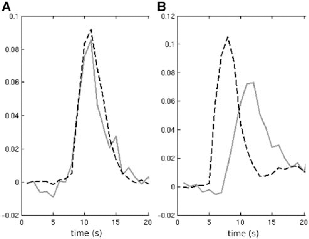
Example LAIF2 time-courses (red) from patients A and K (panels A and B, respectively) together with the GAIF time-course (black dashed). Both are normalized to the first passage. The locations of the local AIF voxels are shown by the crosses in Figure 4. AIF, Arterial Input Function; GAIF, global AIF; LAIF2, local AIF (new method).

To illustrate four different scenarios, data sets A, F, K, and S are shown in Figure 4. Data set A (Figure 4i) illustrates a case where LAIF2 slightly increases the dispersion area compared with the GAIF result (see previous paragraph). The similar perfusion maps may also be inferred from the comparison of the LAIF2 time-courses with the GAIF. In the example shown in Figure 5A, the LAIF2 and GAIF curves show similar characteristics, suggesting the dispersion of blood flow in the smaller feeding arteries is minimal in this case. In data sets F, K, and S, LAIF2 decreased the dispersion area compared with the GAIF result (Δ%abnRTM<0). Data set F (Figure 4ii) illustrates a case where the dispersion area calculated using LAIF2 (%abnRTM_LAIF2=43%IH) is larger than the apparent abnormal perfusion area (%abnMTT_LAIF2=10%IH). However, there is a similar reduction in %abnRTM and %abnMTT achieved by LAIF2 (Δ%abnRTM=−23%IH and Δ%abnMTT=−24%IH) compared with GAIF. This reduction in dispersion lowers the apparent MTT values, and in some areas they fall below the hypoperfusion threshold. Data set K (Figure 4iii) illustrates a case where the LAIF2 dispersion area (%abnRTM_LAIF2=22%IH) is smaller than the apparent abnormal perfusion area (%abnMTT_LAIF2=43%IH), and where LAIF2 achieves a greater reduction in %abnRTM than in %abnMTT (Δ%abnRTM=−35%IH and Δ%abnMTT=−12%IH) compared with the GAIF result. This suggests that the extent of the GAIF hypoperfusion area is fairly reliable (since reducing dispersion (using LAIF2) does not alter the hypoperfused area very much), although its severity is exaggerated by dispersion. The reduction in dispersion error can also be inferred from the comparison of the example LAIF2 time-course with the GAIF (Figure 5B). Since there is delay and dispersion in the feeding arteries, LAIF2 is both delayed and dispersed compared with the GAIF, therefore reducing dispersion error. Data set S (Figure 4iv) illustrates a case where LAIF2 significantly reduces dispersion and apparent hypoperfusion areas (Δ%abnRTM=65%IH and Δ%abnMTT=43%IH) compared with the GAIF results, with similar residual dispersion (abnRTM_LAIF2=17%IH) and apparent hypoperfusion (abnMTT_LAIF2=18%IH) areas. The small residual dispersion suggests that dispersion-induced perfusion errors have been minimized using LAIF2.

Discussion

In this study, we have evaluated two local AIF methods LAIF1 and LAIF2, whose source locations are determined as the local minima of FM_C and FM_adj, respectively. The reduced dependence of FM_adj on MTT is theoretically important for locating local AIF voxels in transition regions between normal and abnormally perfused tissue. However, only a validation of the local AIFs in vivo can elucidate whether the associated loss in precision (see Figure 2) outweighs the MTT insensitivity benefit. The in vivo data reveal that overall the novel LAIF2 method is marginally more successful than LAIF1 in reducing dispersion, suggesting that at times it locates more appropriate local AIFs. In the majority of data sets, LAIF2 reduces both the dispersion and hypoperfusion compare with GAIF, suggesting that overall the local AIFs are performing their theoretical role of reducing dispersion-induced perfusion errors.

The in vivo data in this paper had TR∼2 seconds and contrast-to-noise ratio ∼10 to 20 (peak GM concentration to prebolus baseline SD), for which there was some difficulty in fitting the GV functions for lower contrast-to-noise ratio white matter and ischemic regions. Consequently, in these regions, the local AIFs were taken from neighboring local AIF territories, potentially permitting dispersion error; this would explain the residual dispersion areas with the local AIF methods. The localized MTT and RTM ‘hot spots’ in Figure 4 are attributed to erroneous local AIFs. Such hot spots were more frequent in the white matter regions of LAIF1 maps, possibly due to the MTT dependence of the source locations. The use of better quality data, such as that obtained with the latest generation of MRI scanners or by using the protocol recommended by Knutsson et al (2004), should minimize the GV-related limitations. Furthermore, a 2D (or ideally a 3D) acquisition with isotropic voxels would naturally lend itself to a 3D within-volume search for suitable LAIF voxels, with potential to better localize the LAIF territories.

It should be noted that the parameter and threshold used for dispersion assessment, RTM≥TR, has good specificity but limited sensitivity in detecting dispersion. For example, a voxel with RTM<TR may still have a small dispersion (and therefore contain perfusion error), but it cannot be distinguished from delay (where perfusion is unbiased using oSVD). A more optimized protocol with shorter TR (Wintermark et al, 2008) would minimize this effect. Furthermore, the abnormal perfusion threshold MTT>MTT_contraGM+1.78 seconds was taken from work looking at infarct prediction in acute data (Christensen et al, 2009), and from a GAIF analysis. Because of dispersion, the MTT values obtained with a GAIF analysis may have been overestimated. It follows that for a LAIF analysis where dispersion is minimized, the abnormal MTT threshold may be lower. However, since the duration of ischemia is a significant factor in determining tissue infarction, the threshold with greatest sensitivity and specificity for infarct prediction will probably change with time of scan; and therefore, a time-dependent threshold could be more appropriate for our data. Further work is needed to determine the optimal threshold both for local AIF methods and for different scan times. Nevertheless, the threshold used in this study illustrates the issues of defining the perfusion abnormality using global and local AIF methods.

Although GAIF identified larger areas of hypoperfusion (due to dispersion-related perfusion error), it is necessary to determine whether a different (larger) MTT threshold would identify the same hypoperfused area as identified using LAIF2. If this was the case, the GAIF could still provide the same clinical information. For the data sets in Figure 4ii–iv, we found that a threshold of MTT>MTT_contraGM+n, (where n=3 seconds for data sets F and K and n=5 seconds for data set S), caused the size of the GAIF MTT abnormality to be approximately the same as the reported LAIF2 MTT abnormality using the original MTT>MTT_contraGM+1.78 seconds threshold. Similarly, for the remaining data sets, n ranged from 0 to 5.5 seconds, with a weak indication of higher thresholds in the hyperacute phase. However, n varied significantly for similar time-to-scan values. This suggests that LAIF2 does provide different information regarding the patient's hemodynamic status, and that a single choice of threshold would not be sufficient for the GAIF to give the same results as the LAIF2 method. The unpredictable difference between the severity of the GAIF and LAIF2 hypoperfusion has two causes: first, the degree (extent and severity) of dispersion varied between patients, causing varying degrees of perfusion error with the GAIF; second, in most cases LAIF2 only partially removed the dispersion, and as such is still prone to overestimate MTT in affected regions. The amount of error in the GAIF MTT and the degree of correction obtained in the LAIF2 MTT cannot be known a priori, stressing the difficulty in choosing a hypoperfusion threshold that reflects true perfusion rather than perfusion and dispersion. Thus, the maps in Figure 4 serve only as a guide of abnormality and a useful tool for comparing the GAIF and LAIF2 methods, but are not intended to provide a stand-alone indication of tissue at risk of infarction.

Interestingly, however, a visual comparison of the limited available follow-up data with the initial perfusion abnormality revealed that for all cases the LAIF2 methodology delineates an abnormal perfusion volume that is more closely aligned with the final infarct volume (an example is shown in Figure 6), compared with the much larger GAIF area. This underlines the caution that should be taken when using dispersion-contaminated GAIF perfusion maps to assess for tissue at risk of infarction. However, we acknowledge the very preliminary nature of these findings due to the limited amount of follow-up data available.

Figure 6

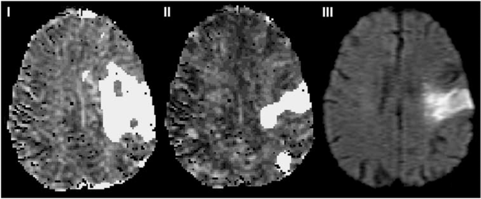
Example of how local AIF methodology may delineate final infarct volume more closely than the standard GAIF method. The left and central maps are MTT with areas of MTT>Thld overlaid in yellow for (i) GAIF and (ii) LAIF2 at acute scan time of 3 hours (data set O, Table 1). The right hand image (iii) is the follow-up 108 day diffusion scan. AIF, Arterial Input Function; GAIF, global AIF; LAIF2, local AIF (new method); MTT, mean transit time; Thld=MTT_contraGM+1.78 seconds (see text).

Several major clinical trials have used the Tmax parameter to identify at-risk tissue (e.g., Albers et al, 2006; Davis et al, 2008). Tmax primarily reflects the delay and dispersion in the supplying vessels, but has only mild dependence on tissue perfusion itself (Calamante et al, 2010). Tmax, however, cannot distinguish delay and dispersion, and the presence of one cannot be inferred from the other (Calamante et al, 2006). Distinguishing any additional risk associated with dispersion separate from delay (and vice-versa) would be valuable information. A generalized linear model (e.g., Wu et al, 2001) that combines delay and dispersion as well as an unbiased perfusion estimate (using, e.g., a validated local AIF methodology and oSVD deconvolution) could help delineate the impact of delay and dispersion on progression of tissue infarction. Work to develop such a predictor model and to further investigate delay and dispersion is in progress.

Due to the long computational time, the owMLEM validation methodology (to measure the residual dispersion) is not practical for use in acute clinical stroke analysis. For this reasons, we used the more conventional and fast oSVD method to calculate FM_adj and LAIF2. However, accurate validation methodology, such as with owMLEM, is an important step for the development and evaluation of local AIF methods. Indeed, the local AIF methods presented here are shown to reduce dispersion, providing a direct assessment of the veracity of their associate perfusion maps.

To conclude, both of the local AIF methods presented here were found to reduce the amount of residual dispersion in the perfusion maps compared with the conventional GAIF analysis. The corresponding reduction in dispersion-related perfusion error suggests that the local AIF methods can better characterize the severity and extent of any perfusion deficit. Of the two local AIF methods, the novel method (LAIF2) was found to be marginally better in reducing dispersion.