Sage Journals: Discover world-class research

Abstract

A strategy for attitude adjustment of a free-floating space robot is proposed to reduce fuel consumption and time required to operate a space manipulator and its carrier before and after the detection of an on-orbit spacecraft. This strategy can be used in such a way that the carrier attitude and space manipulator joint angle reach their expected values at the same time. In order to obtain an advanced effect of carrier attitude adjustment, a novel parameterization method of joint trajectory is proposed, which extends the search scope of the joint trajectory by the fusion of the 4-3-4 and 3-5-3 planning methods. An objective function is defined according to the difference of the expected and initial carrier attitudes. A genetic algorithm is used to search for an optimal solution of the parameters. The effectiveness of the proposed strategy is verified through simulations for a six-degree-of-freedom (6-DOF) space robot system.

Keywords

Space Manipulator Attitude Adjustment Parameterization Function On-orbit Detection Trajectory Planning

1. Introduction

Continuous development of space technologies has led to increasing demand for longer life cycles and higher reliability of future spacecraft. To ensure stable and reliable operation of spacecraft in complicated space environments, on-orbit detection has currently become a key technology for spacecraft fault diagnosis and threat warning. At the same time, in fields such as space assembly, system upgrade and logistic support, on-orbit detection technologies have a wide range of requirements [1]. Research projects, such as the XSS Project [2] and MiniAERCam Project [3], promote the development of relevant technologies in the on-orbit detection field.

Typically, space robots in an orbit have good mobility, flying along with a multiple-DOF manipulator system with sensors [4]. Such a system can be used as a novel platform for detection of spacecraft approaching and flight support. Space robotic technologies are currently being developed by several countries; examples include the Japanese ETS-VII [5], the American Orbital Express [6], and the German Light Weight Robot [7] and ROKVISS [8]. A safe, viable and effective close inspection system for specific detection can be realized using a specially designed space robot, which incorporates various non-contact sensors, such as a laser triangulation sensor mounted on the manipulator end-effector. On-orbit detection is aimed at the surface of the spacecraft structure. For a particular detection task, an on-orbit detection procedure using a space manipulator covers the following four processes [9]. First, the space robot system approaches the spacecraft and moves the space manipulator close to the surface of the spacecraft that needs to be tested. Next, the space manipulator tracks the trajectory and detects the surface that needs to be tested on the spacecraft. The third step is to finish the detection task and berth the manipulator. Lastly, the carrier attitude is re-stabilized.

In order to reduce energy consumption, the attitude control system of the space robot system is usually switched off to allow for a free-floating state [10]. Compared to normal space robot operation, the initial values of the carrier attitude and space manipulator joint angles have significant influence on the detection process. If the initial values of the carrier attitude and manipulator configuration are not appropriate, some parts of the carrier will be too close to the spacecraft, leading to a collision during the detection process when the attitude changes and the space manipulator moves. To minimize the collision probability, the carrier attitude and manipulator configuration need to be adjusted before the operation. After the detection operation, the position and attitude of the carrier change from the initial position and attitude. A change in the carrier attitude directly changes the attitude of the solar panel relative to the Sun and that of the antenna relative to the Earth. This affects the performance of the power and communication system on the space robot. As a result, the entire system needs to be re-stabilized to ensure normal working conditions after detections are completed and the system moves to the corresponding attitude [11]. In other words, before and after the on-orbit detection task, the mechanical arm has to carry out two operations. First, it has to berth the manipulator. This is achieved by re-initializing each joint angel to the initial state. Next, re-stabilization of the attitude for the entire system needs to be carried out. Using the dynamic coupling relationship between the space manipulator and its carrier, combined with the manipulator motion, allows the two operations to be carried out at the same time. This also reduces the time to carry out the operations, while saving valuable fuel carried by the space robot system.

Research reported in the literature has primarily taken advantage of the non-holonomic characteristic of space robots and specific trajectory planning methods employed by space manipulators in order to realize the process of finishing the manipulator movement and carrier attitude re-stabilization at the same time. Vafa et al. [12] proposed a carrier attitude adjustment strategy based on the disturbance map and periodic motion method. This control strategy can be realized by using the motion of the space manipulator when tracking a closed trajectory in the joint space. However, this method requires the total change of the carrier attitude to be an integral multiple of attitude change produced by the space manipulator joint space in each periodic motion. Moreover, this method overlooks non-linearity above two orders. Dubowsky et al. [13] proposed an enhanced disturbance map method that requires a large amount of calculations. Consequently, the method is not accurate when used for carrier attitude adjustment. Suzuki et al. [14] improved the calculus of variations and obtained an optimal spiral trajectory. Any change is recorded in 9D state variables, including the end-effector position and attitude of the space manipulator, together with the attitude of the carrier.

The methods discussed previously cannot be used to make the joint angle of the space manipulator reach the expected value while controlling the carrier attitude. To overcome this issue, Tortopidis et al. [15] proposed an analytical method to drive the system to a desired configuration. This method is based on the mapping of the angular momentum to a space where it can be satisfied trivially. Examples of a 2-DOF free-floating space manipulator are discussed in their work. Xu et al. [16] parameterized the joint trajectory to realize the purpose of the controlling carrier attitude. Their method allows the space manipulator joint angle to reach the expected value. However, due to the limited trajectory searching space of this parameterization method, it has certain limitations related to carrier attitude control.

In this paper, a novel joint trajectory parameterization method based on the task requirements is discussed. This is followed by establishing an optimized objective function, where the purpose of controlling the carrier attitude and making the space manipulator joint angle reach the expected value, is realized using an optimization algorithm. The established parameterization equation extends the searching space of the joint trajectory and enhances carrier attitude adjustment effects of free-floating space robots.

2. Carrier attitude adjustment of a space robot

The vector model of an n-DOF space manipulator motion, based on a free-floating satellite carrier, is shown in Figure 1. C_i is the centroid of the manipulator linkage i; ∑_I and ∑_E are the inertial coordinate system and end-effector coordinate system, respectively; r_i is the position vector of the centroid of the manipulator linkage i in the inertial coordinate system; p_i is the position vector of the joint J_i in the inertial coordinate system; p_e is the position vector of space manipulator end-effector in the inertial coordinate system; a_i is the position vector pointing from joint J_i to C_i; and b_i is the position vector pointing from C_i1 to joint J_i.

Figure 1.

General kinematic model of a free-floating space robot

According to the model, the position vector of the manipulator end-effector can be expressed as follows:

p_{e} = r_{0} + b_{0} + \sum_{i = 1}^{n} (a_{i} + b_{i})

(1)

Linear velocity of the space manipulator end-effector can be obtained by taking the derivative of Equation (1):

v_{e} = {\dot{p}}_{e} = v_{0} + ω_{0} \times (p_{e} - r_{0}) + \sum_{i = 1}^{n} [k_{i} \times (p_{e} - p_{i})] {\dot{θ}}_{i}

(2)

The angular velocity of the end-effector can be expressed as follows:

ω_{e} = ω_{0} + \sum_{i = 1}^{n} k_{i} {\dot{θ}}_{i}

(3)

where v₀ and ω₀ are the carrier mass centre linear and angular velocity relative to the inertial coordinate system, respectively; k_i is the unit vector, reflecting the rotation direction of the joint i; and θ_i is the rotation angle of the joint i. The following expression can be obtained from Equations (1) and (2):

[\begin{array}{l} v_{e} \\ ω_{e} \end{array}] = J_{s} [\begin{array}{l} v_{0} \\ ω_{0} \end{array}] + J_{m} \dot{θ}

(4)

Equation (4) is a general dynamic equation, where the block matrix J_s is the Jacobi matrix related to the carrier motion, while the block matrix J_m is the Jacobi matrix related to the manipulator motion. The corresponding Jacobi matrices of the fixed-base manipulator from J_m and the space manipulator are the same.

During the detection process, to avoid a collision of the space manipulator and spacecraft, and to reduce energy consumption related to attitude adjustment, the system is generally in the state of free-floating; i.e., the position and attitude of the satellite platform as the manipulator carrier is uncontrolled. Non-holonomy is also a characteristic of the system [17]; in other words, the system meets the following two non-holonomic constraints:

\sum_{i = 0}^{n} m_{i} {\dot{r}}_{i} = 0

(5)

\sum_{i = 0}^{n} (I_{i} ω_{i} + r_{i} \times m_{i} {\dot{r}}_{i}) = 0

(6)

According to the above two linear momentum conservation equations, the expression for the carrier linear velocity can be obtained as follows: v ₀, ω ₀:

v_{0} = - (J_{T w} / ω - {\tilde{r}}_{0 g} H_{s}^{- 1} H_{m}) \dot{θ}

(7)

ω_{0} = - H_{s}^{- 1} H_{m} \dot{θ}

(8)

The carrier attitude can be expressed as the integral of $ω_{0}$ ,

B_{ω} (t) = \int_{0}^{t} ω_{0} (t) d t = \int_{0}^{t} - H_{s}^{- 1} H_{m} \dot{θ} (t) d t

(9)

According to the non-holonomic characteristics of the space manipulator, the re-stabilizing carrier attitude and berthing space manipulator can be realized by planning the motion of the manipulator joint. In other words, it is anticipated to reach the expected values of the space manipulator joint angle and carrier attitude at the same time. As singularity does not exist in the motion of joint space planning of the manipulator, this method can be easily realized. The expected carrier attitude can be assumed to be B_d, while the norm is defined as || x || = sqrt( x ^T x ). The optimized objective function of attitude adjustment, then, can be written as follows:

B = ‖ B_{ω} (t_{f}) - B_{d} ‖ + J_{q}

(10)

The bounded variable of the joint motion range J_q is given by the following expression:

J_{q} = {\begin{cases} + \infty θ_{i} > θ_{+ i_\lim i t} \\ + \infty θ_{i} < θ_{- i_\lim i t} \\ 0 θ_{- i_\lim i t} \leq θ_{i} \leq θ_{+ i_\lim i t} \end{cases}

(11)

In the calculation, when the joint angle exceeds the motion range (θ_{-i_limit}, θ_{+i_limit}), J_q is equal to the positive infinity; hence, the optimization algorithm automatically shields trajectories exceeding the joint motion range.

3. Parameterization of the joint trajectory

The motion trajectory in the joint space refers to the displacement, velocity and acceleration curves for each joint of the robot during movement as a function of time. The joint trajectory is required to meet the following boundary conditions:

\begin{array}{l} θ_{i} (0) = θ_{i 0}, θ (t_{f}) = θ_{i e} \\ {\dot{θ}}_{i} (0) = {\ddot{θ}}_{i} (0) = {\dot{θ}}_{i} (t_{f}) = {\ddot{θ}}_{i} (t_{f}) = 0 \end{array}

(12)

In Equation (12), the number of unknown variables is equivalent to that in the constraint condition. Therefore, a parameterization is used to set undetermined parameters in the joint trajectory equation and express other unknown variables with the undetermined parameters according to these boundary conditions. After the joint trajectory is parameterized, different joint trajectories can be obtained by changing undetermined parameters. In the parameterization method, more undetermined parameters can be introduced to obtain a wider searching space of the joint trajectory. However, this would increase the difficulty associated with solving the equation. But, the parameterization method with joint fusion trajectory can be employed to resolve the above contradiction.

Generally, traditional parameterization methods to estimate the joint trajectory can only produce a cluster of trajectory curves for certain specific types with several fixed characteristics. For example, the 4-3-4 planning employs the proportion of quartic polynomials in 4-3-4; namely, the time and displacement are taken as undetermined parameters [18]. The trajectory formed always passes through an intermediate point, which is not dependent on the selection of undetermined parameters.

Based on the traditional trajectory parameterization method, this paper proposes a parameterization method based on the joint fusion trajectory to expand the trajectory search scope. According to this method, the trajectory $S_{i} (t)$ (i=1∼2) includes the undetermined parameters $α_{i}$ and $β_{i}$ . According to the boundary equation, $α_{i}$ and $β_{i}$ are used to express all unknown quantities in the equation $S_{i} (t)$ . Next, parameters $α_{i}$ , $β_{i}$ and $S_{i} (t)$ meet the boundary conditions. Therefore, the following assumption can be made:

S_{3} (t) = A S_{1} (t) + (1 - A) S_{2} (t)

(13)

where A is the parameter to be optimized. Therefore, $S_{3} (t)$ has a total of five parameters that need to be optimized, including $α_{1}$ , $β_{1}$ , $α_{2}$ and $β_{2}$ .

To obtain the parameterization of the equation with the fusion trajectory, the 4-3-4 trajectory planning [18] and 3-5-3 trajectory planning [19] methods are introduced into the parameters that need to be optimized. The same method as discussed above is used to introduce parameters into the two methods. The 3-5-3 planning is provided as an example here (as shown in Figure 2), with the trajectory curve $h_{2} (t)$ in the middle section, which is a quintic polynomial. The initial and final trajectory curves $h_{1} (t)$ and $h_{3} (t)$ are cubic polynomials.

Figure 2.

Trajectory planning using the 3-5-3 method

The total displacement of the joint angle is given by:

h_{f 0} = h_{f} - h_{f 0}

(14)

Parameters d₁, d₂ and d₃ are the angular displacements of the parameterization trajectory in each section, while t₁, t₂ and t₃ are the run-time of the parameterization trajectory also in each section.

In this method, the following undetermined parameters α and β are introduced:

{\begin{cases} α = d_{1} / (h_{f} - h_{0}) \\ β = d_{3} / (h_{f} - h_{0}) \end{cases}

(15)

From this, the joint angular displacement of each section can be expressed as follows:

{\begin{cases} d_{1} = α (h_{f} - h_{0}) \\ d_{2} = (1 - α - β) (h_{f} - h_{0}) \\ d_{3} = β (h_{f} - h_{0}) \end{cases}

(16)

To make the joint trajectory as smooth as possible, the run-time of the polynomial in each section is assumed to be as follows:

{\begin{matrix} t_{1} = | d_{1} | / (| d_{1} | + | d_{2} | + | d_{3} |) \\ t_{2} = | d_{2} | / (| d_{1} | + | d_{2} | + | d_{3} |) \\ t_{3} = | d_{3} | / (| d_{1} | + | d_{2} | + | d_{3} |) \end{matrix}

(17)

After the time in each section is normalized, the following expression is obtained:

{\begin{matrix} t = T / t_{1} \\ t = (T - t_{1}) / t_{2} \\ t = (T - t_{1} - t_{2}) / t_{3} \end{matrix} \begin{matrix} ​ \\ ​ \\ ​ \end{matrix} \begin{matrix} 0 \leq T \leq t_{1} \\ t_{1} < T \leq t_{2} + t_{1} \\ t_{2} + t_{1} < T \leq t_{1} + t_{2} + t_{3} \end{matrix}

(18)

where T is a certain time node in the planning process, with the initial time T assumed to be zero.

The planning trajectory uses the boundary conditions, where the initial angle h₀, initial velocity v₀, initial joint angular acceleration a₀, objective joint angle h_f, objective velocity v_f and objective acceleration a_f are all zero.

After the above conditions are substituted into Equation (12), the following polynomial equations for each of the three sections are obtained.

The cubic polynomial equation for the first section is given by:

\begin{array}{l} h_{1} (t) = (d_{1} - v_{0} t_{1} - a_{0} t_{1} ​^{2} / 2) t^{3} + (a_{0} t_{1} ​^{2} / 2) t^{2} \\ + (v_{0} t_{1}) t + h_{0} \\ v_{1} = {\dot{h}}_{1} (1) / t_{1} = 3 δ_{1} / t_{1} - 2 v_{0} - a_{0} t_{1} / 2 \\ a_{1} = {\ddot{h}}_{1} (1) / t_{1}^{2} = 6 d_{1} / t_{1} ​^{2} - 6 v_{0} / t_{1} - 2 a_{0} \end{array}

(19)

The quintic polynomial equation for the second section is given by:

\begin{array}{l} h_{2} (t) = (6 d_{2} - 3 v_{1} t_{2} - 3 v_{2} t_{2} - a_{1} t_{2} ​^{2} / 2 + a_{2} t_{2} ​^{2} / 2) t^{5} \\ + (- 15 d_{2} + 8 v_{1} t_{2} + 7 v_{2} t_{2} + 3 a_{1} t_{2} ​^{2} / 2 - a_{2} t_{2} ​^{2}) t^{4} \\ + (d_{1} - v_{0} t_{1} - a_{0} t_{1} ​^{2} / 2) t^{3} + (a_{0} t_{1} ​^{2} / 2) t^{2} \\ + (v_{0} t_{1}) t + h_{0} \\ v_{2} = 3 d_{3} / t_{3} - 2 v_{f} + a_{f} t_{3} / 2 \\ a_{2} = - 6 d_{3} / t_{3} ​^{2} + 6 v_{f} / t_{3} - 2 a_{f} \end{array}

(20)

The cubic polynomial equation for the third section is given by:

\begin{array}{l} h_{3} (t) = (d_{3} - v_{f} t_{3} + a_{f} t_{3} ​^{2} / 2) (t - 1)^{3} \\ + (a_{f} t_{3} ​^{2} / 2) (t - 1)^{2} + v_{f} t_{3} (t - 1) + h_{f} \end{array}

(21)

In terms of the trajectory parameterization using the 4-3-4 method, the above method can be used to introduce the undetermined parameters $α'$ and $β'$ , and the parameterization equation $S_{2} (t)$ is as follows.

The quartic polynomial trajectory in the first section is given by:

\begin{array}{l} h_{1} (t) = (d_{1} - v_{0} t_{1} - a_{0} t_{1} ​^{2} / 2 - σ) t^{4} + σ t^{3} \\ + (a_{0} t_{1} ​^{2} / 2) t^{2} + (v_{0} t_{1}) t + h_{0} \\ v_{1} = {\dot{h}}_{1} (1) / t_{1} = 4 d_{1} / t_{1} - 3 v_{0} - a_{0} t_{1} - σ / t_{1} \\ a_{1} = {\ddot{h}}_{1} (1) / t_{1} ​^{2} = 12 d_{1} / t_{1} ​^{2} - 12 v_{0} / t_{1} - 5 a_{0} - 6 σ / t_{1} ​^{2} \end{array}

(22)

where $σ = f / g$ , f and g are expressed as follows:

\begin{array}{l} f = 2 d_{1} (4 + 2 t_{3} / t_{2} + 2 t_{3} / t_{1} + 3 t_{2} / t_{1}) \\ - (d_{2} t_{1} / t_{2}) (3 + t_{3} / t_{2}) \\ + 2 d_{n} t_{1} / t_{n} - v_{f} t_{1} - v_{0} t_{1} (6 + 6 t_{2} / t_{1} + 4 t_{3} / t_{1} + 3 t_{3} / t_{2}) \\ - a_{0} t_{1} t_{3} (5 / 3 + t_{1} / t_{2} + 2 t_{1} / t_{3} + 5 t_{2} / 2 t_{3}) + a_{f} t_{1} t_{3} \\ g = t_{3} / t_{2} + 2 t_{3} / t_{1} + 2 + 3 t_{2} / t_{1} \end{array}

(23)

The cubic polynomial trajectory in the second section is given by:

\begin{array}{l} h_{2} (t) = (d_{2} - v_{1} t_{2} - a_{1} t_{2} ​^{2} / 2) t^{3} + (a_{1} t_{2} ​^{2} / 2) t^{2} \\ + (v_{1} t_{2}) t + h_{1} (1) \\ v_{2} = {\dot{h}}_{2} (1) / t_{2} = 3 d_{2} / t_{2} - 2 v_{1} - a_{1} t_{2} / 2 \\ a_{2} = {\ddot{h}}_{2} (1) / t_{2} ​^{2} = 6 d_{2} / t_{2} ​^{2} - 6 v_{1} / t_{2} - 2 a_{1} \end{array}

(24)

The quartic polynomial trajectory in the third section is given by:

\begin{array}{l} h_{3} (t) = (9 d_{3} - 4 v_{2} t_{3} - a_{2} t_{3} ​^{2} / 2 - 5 v_{f} t_{3} \\ + a_{f} t_{3} ​^{2} / 2) t^{4} + (- 8 d_{3} + 5 v_{f} t_{3} - a_{f} t_{3} ​^{2} / 2 \\ + 3 v_{2} t_{3}) t^{3} + (v_{2} t_{3} ​^{2} / 2) t^{2} + (v_{2} t_{3}) t + h_{2} (1) \end{array}

(25)

After trajectories $S_{1} (t)$ and $S_{2} (t)$ are combined, the undetermined parameter A is introduced to obtain the parameterization trajectory equation $S (t)$ with a single joint as follows:

S (t) = A S_{1} (t) + (1 - A) S_{2} (t)

(26)

The equation $S (t)$ covers five undetermined parameters, namely $α'$ , $β'$ , α, β and A, where the values of the first four parameters vary between $- 0.5 \sim 0.5$ , while A varies between $- 0.5 \sim 1.5$ .

4. Carrier attitude/adjustment control method

Genetic algorithms (GAs) have excellent global optimization performance. Therefore, the method is more advantageous in comparison to the traditional Gradient Method [20] allowing the optimization of multiple variables.

A GA is employed in this paper to realize the carrier attitude adjustment with the aim of resolving problems associated with trajectory planning in order to adjust the carrier attitude and berth the space manipulator. The following steps are used to implement the GA:

The initial population of undetermined parameters in the parameterization equation related to each joint is generated. In the parameter search scope, for each joint, the initial population of undetermined parameters ( $α'$ , $β'$ , α, β and A) includes N randomly generated individuals. In other words, N initial motion trajectories are generated.

Fitness function in the GA is assumed to be the optimized objective function B. In turn, according to Equation (10), the fitness of each individual in the population is calculated.

The classic roulette algorithm is used as the selection method in the GA. The probability of the individual selection is given by:

P_{i} = \frac{f_{i}}{\sum_{k = 1}^{M} f_{k}}

(27)

where M is the population and f_i is the adaptability of individual i.

Two individuals are randomly selected after the selection algorithm. Next, an intersection position is arbitrarily chosen for exchanging parts of the genetic code to form two new individuals.

According to the mutation probability, the genetic code of a certain individual in the population can be altered by taking the inverse with a small probability.

A new population is generated from the offspring.

Steps from (b) to (f) are repeated until an optimal solution meeting the requirements is obtained.

5. Simulations

As shown in Figure 3, according to the configuration when each joint angle in a 6-DOF space manipulator is equal to zero, the coordinate system of the free-floating space robot is established as shown in Figure 3.

Figure 3.

Linkage coordinate frames for a 6-DOF manipulator

The coordinate system {1} linked with the linkage i is defined in the position of the joint i (the joint closest to the carrier is defined as joint 1), and Z-axis in the coordinate system is defined as the joint rotation axis. Structural parameters along with the mass and inertia of each linkage are listed in Table 1. Parameter a ₀ is the position vector from the original point in the inertial coordinate system to the carrier centroid. The original point in the inertial coordinate system is chosen to coincide with the centroid of the carrier; i.e., the position a ₀ corresponds to (0, 0, 0). Parameter b ₀ is the position vector from the centroid of the carrier in the inertial coordinate system to the original point of the coordinate system {1}, where a _i ( $1 \leq i \leq 6$ ) is the position vector from the original point in the coordinate system {i} to the centroid of the linkage i, and b _i ( $1 \leq i \leq 5$ ) is the position vector from the centroid of the linkage i in the coordinate system {i} to the original point of the coordinate system {i+1}. Parameter b ₆ is the position vector in the coordinate system {6} for the linkage 6 to the original point in the coordinate system of the space manipulator end-effector.

Table 1.

Linkage parameters of the space robot

Parameters		Carrier	Linkage 1	Linkage 2	Linkage 3	Linkage 4	Linkage 5	Linkage 6
Mass(kg)		450.0	1.5	9.6	1.5	9.0	1.5	10.5
a_i (mm)		0	0	−492.5	0	292.0	0	−136.0
		0	0	54.0	−121.0	−150.0	121.0	0
		0	124.0	0	0	0	0	0
b_i(mm)		500.0	0	−492.5	124.0	349.0	−124.0	−164.0
		0	121.0	−54.0	0	29.0	0	0
		751.0	0	0	0	0	0	0
Moment of inertia (kg/m²)	I_xx	200.00	3.31×10⁻³	3.10×10⁻²	3.31×10⁻³	0.73	3.31×10⁻³	0.10
	I_yy	200.00	3.31×10⁻³	1.50	3.31×10⁻³	0.60	3.31×10⁻³	0.10
	I_zz	200.00	3.31×10⁻³	1.48	3.31×10⁻³	0.63	3.31×10⁻³	0.09
	I_xy	0	0	0	0	0	0	0
	I_xz	0	0	0	0	0	0	0
	I_yz	0	0	0	0	−0.01	0	0

In the simulation, the initial value of the joint angel was (175°, −40°, −120°, 0°, 220°, 0°) and the expected value was (160°, 0°, −80°, 20°, 260°, −20°). The motion range of each joint angle was:

\begin{array}{l} 0^{\circ} \leq θ_{1} \leq 350^{\circ}, - 180^{\circ} \leq θ_{2} \leq 30^{\circ}, \\ - 160^{\circ} \leq θ_{3} \leq 160^{\circ}, - 150^{\circ} \leq θ_{4} \leq 150^{\circ}, \\ 0^{\circ} \leq θ_{5} \leq 350^{\circ}, - 150^{\circ} \leq θ_{6} \leq 150^{\circ} . \end{array}

(28)

Example 1: Global undisturbed attitude optimization.

The optimization objective for the space robot in this example is to move in the joint space from the initial position to the expected position with the attitude of the robot carrier unchanged after the motion is completed. The resulting optimized parameters are shown in Table 2:

Table 2.

Results of the global undisturbed attitude optimization

	A	$α'$	$β'$	α	β
Joint 1	−0.103	0.037	−0.263	−0.095	0.278
Joint 2	−0.329	−0.457	−0.305	−0.383	0.329
Joint 3	0.045	−0.072	−0.232	0.337	0.298
Joint 4	−0.329	0.492	0.064	0.375	−0.107
Joint 5	1.337	0.438	−0.383	−0.430	0.422
Joint 6	0.893	−0.418	0.313	0.138	0.080

According to the optimized parameters, the curves of each joint angle and carrier attitude disturbance can be obtained; they are shown in Figures 4 and 5.

Figure 4.

Joint angle curves of the global undisturbed attitude optimization

Figure 5.

Carrier attitude curves of the global undisturbed attitude optimization

For better visualization of the moving process related to the space robot, a 3D graphic simulation was made based on the results. This 3D simulation is illustrated in Figure 6.

Figure 6.

3D image illustrating undisturbed attitude optimization

Example 2: Attitude adjustment optimization.

The optimization objective for the robot in this example is to move in the joint space from the initial position to the expected position, with the requirement that the attitude of the robot is maintained at the expected value after the motion is completed. The initial attitude of the carrier is (0°, 0°, 0°) and the expected attitude is (5°, 5°, 5°).

Optimized parameters are shown in Table 3:

Table 3.

Optimization results of carrier attitude adjustment

	A	$α'$	$β'$	α	β
Joint 1	1.064	0.064	0.185	0.014	−0.064
Joint 2	0.255	−0.488	0.169	−0.088	0.053
Joint 3	−0.119	0.469	−0.337	−0.356	−0.138
Joint 4	0.807	0.313	−0.002	−0.313	0.076
Joint 5	0.893	0.411	0.115	−0.411	0.442
Joint 6	0.823	−0.130	−0.368	−0.438	−0.442

According to the optimized parameters, the curves of each joint angle and carrier attitude disturbance can be obtained; they are shown in Figure 7 and Figure 8.

Figure 7.

Joint angle curves of carrier attitude adjustment

Figure 8.

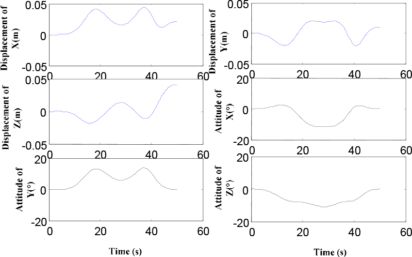
Carrier position and posture curves of carrier attitude adjustment

A 3D image illustrating the results is shown in Figure 9.

Figure 9.

3D image illustrating attitude control/adjustment optimization

Based on the above simulation, it can be seen that, when the space manipulator moves after 50 seconds, the joint angle and carrier attitude reach the expected values, together with a small change in the carrier position.

In order to compare the proposed method using simulation, a trapezoidal speed trajectory planning method in the joint space is introduced. Joint angle curves are shown in Figure 10.

Figure 10.

Joint angle curves of the trapezoidal speed trajectory planning method

After the attitude disturbances in three directions from three trajectories are composed and taken with the absolute values, the measured values of the carrier attitude change can be obtained, as shown in Figure 11.

Figure 11.

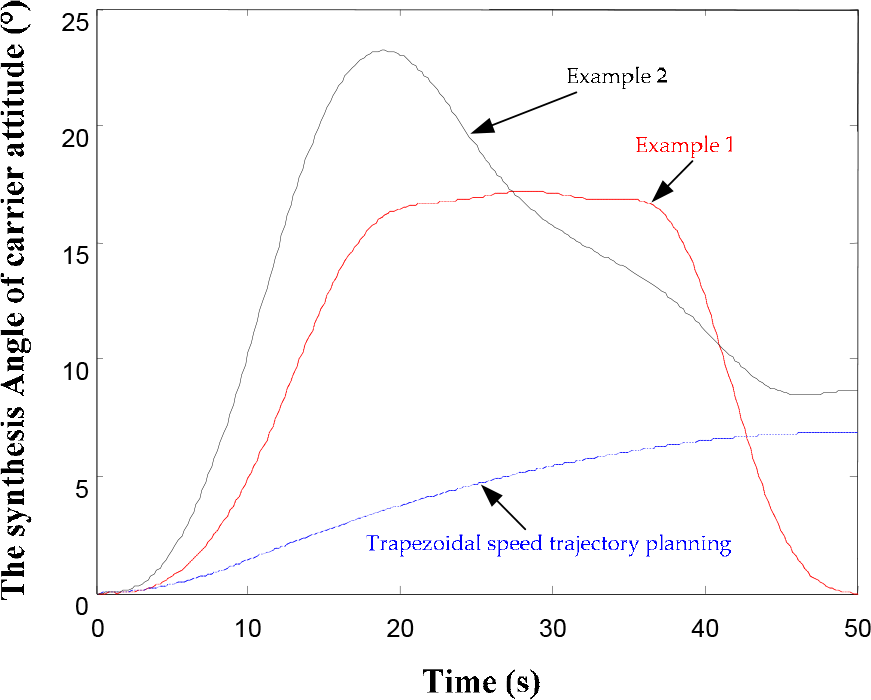
Comparison of measured values of carrier attitude disturbance for each trajectory

In Figure 3, group carrier attitude disturbances are compared during the movement from the initial joint angle (175°, −40°, −120°, 0°, 220°, 5°) to the final joint angle (160°, 0°, −80°, 20°, 260°, −20°). The trajectory produced by the undisturbed attitude optimization of the global attitude of robots was realized with no disturbance of the carrier attitude when the joint angle reached the expected values. The joint motion planned by the attitude adjustment optimization resulted in the final attitude of the carrier reaching the expected value (5°, 5°, 5°), with the adjustment value of the carrier attitude reaching 8.660°. This proved the effectiveness of the joint space parameterization equation and the proposed optimization algorithm.

Regarding the joint trajectory discussed in the above examples, the global attitude disturbance using the trapezoidal planning allowed the attitude disturbance to reach peak value. However, in the two optimization examples, the carrier attitude first generated a peak and then dropped down to zero or the expected attitude. The peak value disturbance of the optimized trajectory far exceeded the trapezoidal planning. This is consistent with the optimized objective function in the paper, which only focuses on the final carrier attitude and does not consider the carrier attitude disturbance during the movement. Accordingly, if the carrier attitude peak value disturbance optimization is needed, it is not enough for the optimized objective function only to include the global attitude. Instead, the peak value should be added into the objective function after introducing corresponding weight coefficients to limit the peak value disturbance. This is done at the expense of the control ability of the global carrier attitude.

The initial and objective configurations of the space manipulator are the same in these three examples. In other words, the displacement in the joint space is the same, yet there are different disturbances in the final carrier attitudes. This also shows that, when the free-floating space robot moves in the joint space, the disturbance of the carrier attitude is related to the movement history.

6. Conclusions

In this paper, a strategy for the carrier attitude adjustment of a space manipulator for on-orbit detection is proposed. A joint trajectory planning method is also proposed, and the objective function is established to reflect the difference in the expected and initial carrier attitudes. The limits of the joint motion range are considered. This algorithm can be used to enable the carrier attitude and space manipulator joint angle to reach their expected values at the same time.

This paper further proposed a novel parameterization algorithm to achieve trajectory planning based on the traditional 3-5-3 and 4-3-4 planning methods. This method allows trajectory selection for a wider search scope, as well as improved optimization. Using simulations for a 6-DOF space manipulator with a free-floating carrier, the effectiveness along with the validity of the carrier adjustment algorithm were verified.

Footnotes

7. Acknowledgements

This work was supported by the National Natural Science Foundation (grant no. 51205090), the Fundamental Research Funds of the Central Universities (grant no. HIT.NSRIF.2015008), the China Postdoctoral Science Foundation (CPSF) (grant no. 2014M551231), and the Heilongjiang Postdoctoral Fund (grant no. LBH-Z12131).

References

Shi

J W

Cai

Y W

Research Summarizing of On-Orbit Testing[J]. Ordnance Industry Automation. 2011,30(6):59–62+83

Madison

R W

. Micro-Satellite Based, On-orbit Servicing Work at the Air Force Research[C]//Aerospace Conference Proceedings, 18–25 March 2000, Big Sky, MT: IEEE; 2000. p. 215–226. DOI: 10.1109/AERO.2000.878421

Fredrickson

S E

Duran

Mitchell

J D

. MiniAERCam Inspection Robot for Human Space Missions[C]//Space 2004 Conference and Exhibit, 28–30 September 2004, San Diego, California:2004. DOI: 10.2514/6.2004-5843

King

Space servicing: past, present and future[C]//Proceedings of the 6th International Symposium on Artificial Intelligence and Robotics & Automation in Space: i-SAIRAS, 18–22 June 2001, Quebec, Canada:2001.

Yoshida

Engineering test satellite VII flight experiments for space robot dynamics and control: theories on laboratory test beds ten years ago, now in orbit[J]. International Journal of Robotics Research. 2003, 22(5):321–335. DOI: 10.1177/0278364903022005003

Wilson

J R

. Satellite Hopes Ride On Orbital Express: DARPA Plans to Extend the Lives of Satellites Already in Orbit by Refueling and Upgrading Them in Space[J]. Aerospace America. 2007, 45(2):30–35

Hirzinger

Sporer

Albu-Schaffer . DLR's Torque-Controlled Light Weight robot III—Are We Reaching the Technological Limits Now[C]//Proceedings of the IEEE International Conference on Robotics and Automation. May, Washington: IEEE; 2002. p. 1710–1716. DOI:10.1109/ROBOT.2002.1014788

Landzettel

Preusche

Albu-Schaffer

Reintsema

Robotic on-orbit servicing-DLR's experience and perspective[C]//Proceedings of the IEEE/RSJ International Conference on Intelligent Robots and Systems.9-15 October 2006, Beijing: IEEE; 2006. p. 4587–4594. DOI: 10.1109/IROS.2006.282164

W F

Liang

. Target berthing and base reorientation of free-floating space robotic system after capturing[J]. Acta Astronautica. 2009, 64(2): 109–126. DOI:10.1016/j.actaastro.2008.07.010

10.

Wayer

K J

Castet

J F

Saleh

J H

. Spacecraft attitude control subsystem: reliability, multi-state analyses and comparative failure behavior in LEO and GEO[J]. Acta Astronautica. 2013, 85(3):83–92. DOI: 10.1016/j.actaastro.2012.12.003

11.

Tortopidis

Papadopoulos

On point-to-point motion planning for underactuated space manipulator systems. Robotics and Autonomous Systems[J]. 2007,55(2):122–131. DOI:10.1016/j.robot.2006.07.003

12.

Vafa

Dubowsky

On the dynamics of space manipulator using the virtual manipulator with application to path planning[J]. The Journal of the Astronautical Science. 1991, 38(4):441–472. DOI: 10.1007/978-1-4615-3588-1_3

13.

Dubowsky

Papadopoulos

The kinematics, dynamics, and control of free-flying and free-floating space robotic systems[J]. IEEE Transactions on Robotics and Automation. 1993, 9(5):531–543. DOI: 10.1109/70.258046

14.

Suzuki

Nakamura

Planning spiral motion of nonholonomic space robots[C]//IEEE International Conferences on Robotics and Automation.22-28 April 1996, Minneapolis, MN:IEEE; 1996. p. 718–725. DOI:10.1109/ROBOT.1996.503859

15.

Papadopoulos

Tortopidis

Nanos

Smooth planning for free-floating space robots using polynomials[C]//Proceeding of the IEEE International Conference on Robotics and Automation. 18–22 April 2005, Barcelona, Spain: IEEE; 2005. p. 4272–4277. DOI: 10.1109/ROBOT.2005.1570777

16.

W F

Liang

Qiang

Non-holonomic Path Planning of Space Robot Based on Genetic Algorithm[C]//Proceedings of the IEEE International Conference on Robotics and Biomimetics. 17–20 December 2006, Kunming, China:IEEE; 2006. p. 1471–1476. DOI: 10.1109/ROBIO.2006.340146

17.

W F

Liang

Survey of modeling, planning, and ground verification of space robotic systems[J]. Acta Astronautica. 2011, 68: 1629–1649. DOI: 10.1016/j.actaastro.2010.12.004

18.

K Y

Liu

M S

. Planning of Sagittal Gait of Biped Robots Based on Minimum Motion Energy[J]. International Journal of Humanoid Robotics. 2010,7(4):635–667. DOI:10.1142/S0219843610002271

19.

Shi

S C

J W

Cui

P Y

Liu

Global Reaction Optimization of Space Manipulator and its Ground Test[J]. Robot. 2009,31(3):242–247+253

20.

Mehrafsa

Sokhandan

Karimian

A High Performance Genetic Algorithm Using Bacterial Conjugation Operator (HPGA)[J]. Genetic Programming and Evolvable Machines. 2013, 14(4): 395–427. DOI: 10.1007/s10710-013-9185-x

Carrier Attitude Adjustment Strategy of a Space Robot for On-Orbit Detection

Abstract

Keywords

1. Introduction

2. Carrier attitude adjustment of a space robot

3. Parameterization of the joint trajectory

4. Carrier attitude/adjustment control method

5. Simulations

6. Conclusions

Footnotes

7. Acknowledgements

References