
Abstract
Aiming at carrying a heavy payload to a desired pose (including position and orientation), a multi-objective optimization-based approach for maximum-payload trajectory planning of free-floating space manipulators (FFSM) is proposed in this paper. The presented approach corresponds to two typical applications: (i) the manipulator joints attain the desired states; (ii) the inertial pose of the end-effector (pose with respect to the inertial frame) attains the desired values, for which a novel two-stage method is presented. Firstly, for the purpose of reducing computational complexity, dynamics equations are derived using a spatial operator algebra (SOA) method. Secondly, objective functions are defined according to the improvement of load-carrying capacity and pose requirements of the end-effector. Then, the joint trajectories are specified using sinusoidal polynomial functions. Finally, a multi-objective particle optimization (MOPSO) algorithm is employed to obtain a non-dominated solution set, during which process particles that do not satisfy the constraints are eliminated. Simulations are performed for a 7-DOF FFSM, considering three and five objectives for optimization in the two applications, respectively. The results demonstrate that the proposed approach can provide satisfactory joint trajectories and improve load-carrying capacity effectively.
Keywords
Introduction
In recent years, space manipulators have been playing increasingly important roles in space exploration, especially in on-orbit payload-carrying operations for large structures in motion. Space manipulators are indispensable during construction and maintenance on the space station [1], capturing of objective satellites [2] and servicing of non-cooperative spacecraft [3], for they can assist or even replace astronauts. Considering the limitation of the load-carrying capacity of space manipulators, excessively heavy payload may not only challenge the capability of joints but also result in instability of the base in the free-floating mode. Therefore, in order to avoid the mentioned problems as far as possible, it is necessary to determine the optimal trajectory which can improve the load-carrying capacity of the FFSM.
Load-carrying capacity is usually defined as the maximum payload that the manipulator can repeatedly lift, and it depends on the dynamic motion or trajectory of the end-effector [4]. The previous studies in this field can be categorized into two groups [5]: the first group aims to determine the DLCC (dynamic load-carrying capacity) and corresponding joint trajectories of redundant manipulators along the given path of the end-effector, calculated considering the limitations of joint torques and tracking error [6,7]; the second group aims to solve the optimal-trajectory-planning problem for manipulators in point-to-point tasks, in which joint trajectories that allow the maximum payload to be carried are determined [8–15]. In order to carry a heavy payload to a desired pose, the second type of problem is considered in this paper.
Most of the previous works on trajectory planning during the load-carrying process have been carried out for ground manipulators. Wang and Ravani (1988) adopted an ILP (iterative linear programming) method to solve the constrained nonlinear optimization problem, synthesizing point-to-point dynamic motions with optimum load-carrying capacities for manipulators [8]. A similar computational technique was developed for obtaining optimal trajectory of wheeled mobile manipulators for a given two-end-point task, in which an extended Jacobian matrix concept was used to solve the redundancy and non-holonomic constraints [9,10]. Korayem and Nikoobin (2008) formulated maximum-payload trajectory planning as an optimal control problem, and the application of Pontryagin's minimum principle resulted in a two-point boundary value problem (TPBVP), which was solved numerically by indirect solution of the optimal control problem [11]. Considering payload constraints, Saravanan et al. (2008) presented a new general methodology, in which optimal trajectory planning of a PUMA560 robot was obtained by evolutionary computation of an elitist non-dominated sorting genetic algorithm (NSGA-II) and differential evolution (DE), respectively [12]. Saramago and Ceccarelli (2002) formulated optimal trajectory planning as subject to physical constraints, input torque/force constraints and payload constraints, while the energy of actuators was considered an objective function [13]. Wang et al. (2001) used the dynamics to produce motions that improve the payload capability, and a point-to-point weightlifting motion planner for a PUMA762 robot was developed by converting the governing optimal-control problem into a direct SQP parameter-optimization problem, in which torque limits were formulated as soft constraints that were added into the objective function [14]. In order to determine optimal trajectory of FFSM in a point-to-point task, Jia et al. (2013) proposed a path-planning method to achieve the goal of payload maximization, in which payload-carrying capacity was improved by minimizing the joint torques [15].
However, essentially the studies mentioned above are single-objective optimization problems. The common ground of these studies is merely that they aim to improve load-carrying capacity through optimizing either mechanical energy of the actuators [11–13] or maximum/minimum value of joint torques [8–10,14,15], which are both crucial objects. In addition, when carrying a heavy payload, free-floating mode is necessary to save the fuel of the spacecraft [16]. The resulting non-holonomic constraint (due to the non-integrability of angular momentum) can introduce the disturbance of base attitude during on-orbit operation process [17], and the influence on load-carrying capacity of FFSM cannot be ignored [18]. According to the analysis above, it is indicated that the multi-objective optimization problem (MOP) needs to be solved during trajectory planning.
It is worth noting that multi-objective trajectory-planning problems of manipulators are usually converted into single-objective problems by using a weighting method [12,19–21], which sometimes tends to be trapped in local optimal solution. Besides this, constantly adjusting the weighting coefficients can consume a large amount of computation time. To solve this problem, multi-objective evolutionary algorithms have been adopted in previous studies for mobile and industrial manipulators [22–24], which are also applicable to trajectory optimization of FFSM. To improve load-carrying capacity of free-floating space manipulators through simultaneous minimization of joint torques, base disturbance and total energy, Liu et al. (2014) proposed a MOPSO-algorithm-based load-maximization trajectory-optimization method [25], which has limitations in the following aspects: (i) only the load-carrying process of a 3-DOF planar manipulator is considered, and trajectory planning of FFSM with higher degrees of freedom in the three-dimensional space is more complicated; (ii) the simulations focus on explaining the optimization of joint torques and base disturbance, without adequately illustrating the results of MOP for all three objectives; (iii) computational efficiency of the proposed algorithm is significantly restricted owing to computation complexity of Newton-Euler dynamics equations and redundancy of some constraint functions. Therefore, further research is necessary.
This paper is organized as follows. Section 2 derives the kinematics and dynamics equations of FFSM with a payload; Section 3 formulates the trajectory-planning problem as a constrained MOP, in which constraints and objective functions are proposed; Section 4, explains the procedure of trajectory planning algorithm using MOPSO. Section 5 shows the simulation results. Section 6 presents the conclusions of the work.
Mathematical model of FFSM with a payload
As shown in Figure 1, the system considered in this paper consists of abase (link n + 1), a revolute-jointed manipulator (from link n to link 1) which has n degrees of freedom, and a payload which is attached to the end-effector. It is assumed that the components of the system are all rigid bodies. Link 1 and payload can be treated as a single composite rigid body, defined as the coordinate system at its mass centre. Mass and inertia tensor of the composite body can be easily obtained as:
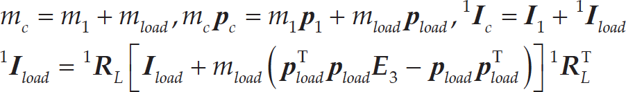
where m
load
and m
c
denote the mass of payload and the composite body, respectively;
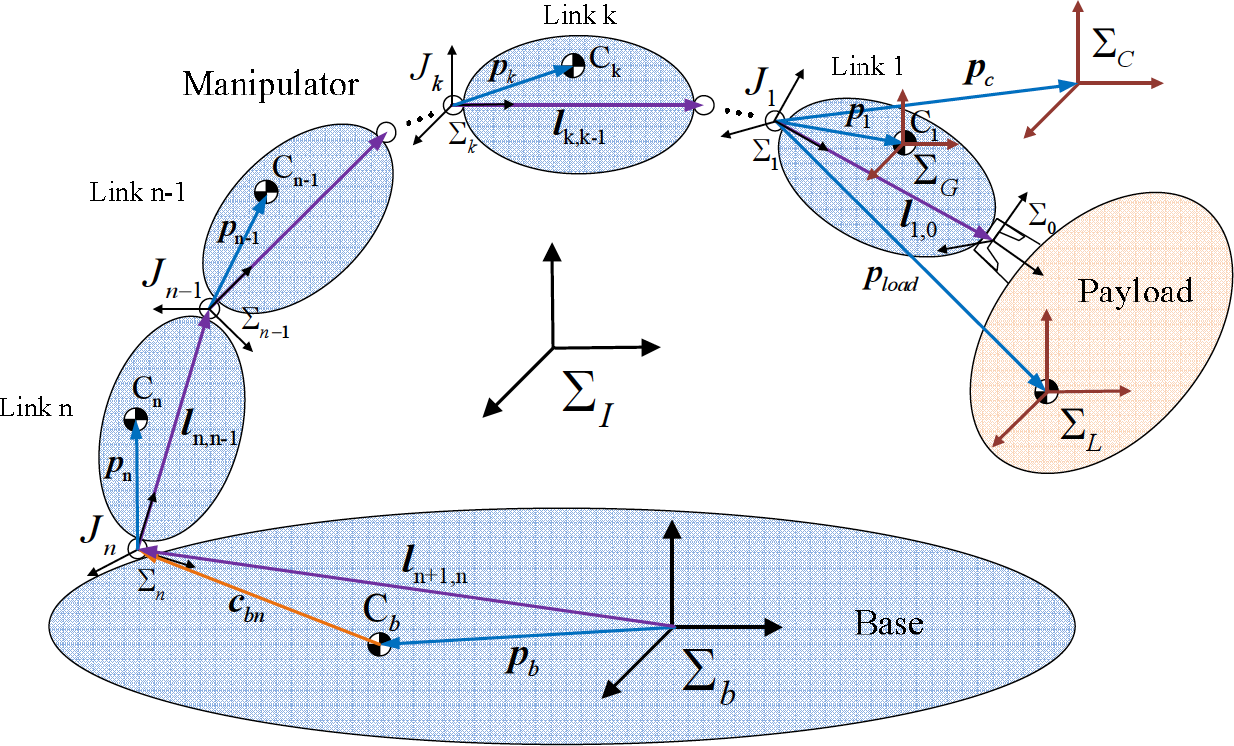
Simplified model of free-floating space manipulators
Define the symbols as follows:
Σ I : inertial coordinate system, which is the reference coordinate system of all recursive calculations;
Σ b : coordinate system of the base;
Σ k : coordinate system of link k(k=n, n−1,…, 1);
Σ G : coordinate system at the mass centre of link 1;
Σ L : coordinate system at the mass centre of payload;
J k . joint k of the manipulator, which is used to connect link k+1 with link k;
C k . mass centre of link k;
m k : mass of link k;
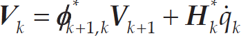
According to [26], the general kinematics equation of space manipulators can be written as:
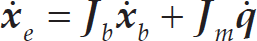
where
It is assumed that the initial linear and angular momentum are equal to zero, and no external forces or torques act on the whole system in the free-floating mode. According to conservation of momentum and angular momentum, we can easily obtain that:

where

where
According to Eq. (4), we have:

According to the SOA method [27], recursive computation of forces and torques from link k + 1 to link k can be achieved using the spatial transferred operator as follows:
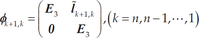
where ∼ denotes that
We define the state-transition matrix of joint k as H
k
= [
The acceleration of link k can be obtained by the differential of Eq. (7):

where
Then, the inertial forces and torques of each link can be computed recursively from link 1 to link n. The spatial inertial

For k = 1, 2, Ȇ n, the spatial force of each link can be computed as follows:

where

The disturbing forces and torques of the base caused by manipulator movement are computed as:

As formulated in Eq. (1), mass and inertia tensor of the composite body can be very large when carrying a heavy payload. According to the dynamics of FFSM, three aspects should be given great importance when executing given joint trajectories (in contrast with identical operation under light payload condition): first, larger driving torques need to be provided, which challenges the capability of the joints; second, larger disturbance force and torques of the base enlarge the range of movement, thus leading to more fuel consumption to maintain position and orientation; and, third, the total kinetic energy of the whole system increases, which will consume large amounts of energy provided by active forces/torques (only joint torques in this study) according to the principle of the conservation of energy. Therefore, limitations of joint driving torques, disturbance of the base, and total energy of the whole system will restrict the load-carrying capacity of FFSM.
According to the analysis above, payload maximization of FFSM can be solved as an MOP, which in this paper emphatically considers minimization of joint torques, base disturbance and total energy. Meanwhile, for a given trajectory, load-carrying capacity can also be affected by configurations of the manipulator, mechanical limit of joints, etc., which are usually regarded as constraints in previous studies. Considering constraints in the load-carrying process, a mathematical model of the constrained MOP can be established.
MOP Statement of Trajectory Planning
In this paper, two different types of boundary value problems are considered: the first challenge is to attain the final desired states of the manipulator joints in joint space (which is equivalent to reaching the desired pose of the end-effector with respect to the base) within the specified time and simultaneously maximize the load-carrying capacity of the FFSM; the second challenge is to reach the final desired pose of the end-effector in the Cartesian space (in the inertial frame) within the specified time and simultaneously maximize load-carrying capacity. In practical engineering, when assembling capsules or extravehicular large-scale equipment on the space station, replacing battery packs and experimental modules, or carrying heavy cargo to specified freight compartments, operations in joint space are needed. When putting a payload into a desired orbit, separating the orbiter, or maintaining spacecraft hover, operations in the inertial frame are needed.
Without loss of generality, we define Δt as the step size and t0 and t f as the initial and final time, respectively; then, the planning steps can be computed as s = (t f −t0)/Δt. Using MOP theory, the FFSM trajectory-optimization problem for the mentioned two types of operations is presented as:
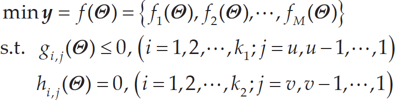
where
The initial and desired joint angle/velocity/acceleration constraints (v=n) are:

Joint angle constraints for t r ∊ [t0, t f ](u=n) are:

Velocity constraints of the end-effector (u=3) are:

For the second type of operation, position- and orientation-deviation constraints of the end-effector (u=6) are:

where Δ
In order to improve the FFSM load-carrying capacity, joint driving torques, disturbance of the base and total energy involved in the motion need to be minimized simultaneously for the first type of challenge. In addition, for the second type of challenge, desired inertia pose of the end-effector should be satisfied when the task is completed. Therefore, five objective functions are established as follows.
Joint driving torques
According to [4], the limitation of joint driving torques would directly restrict the load-carrying capacity of manipulators. For a given payload-carrying task, space manipulators can be enabled to carry a heavier payload by reducing the peak value of joint torques. Therefore, the objective function minimizing joint driving torques is defined as:

When the boundary value of planning is determined, space manipulators can carry a heavier payload with the same fuel consumption for attitude maintenance if an appropriate trajectory is chosen minimizing the disturbance of the base [18]. Defining
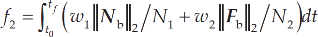
where
Total energy involved in the motion may significantly increase when f1 or f2 is optimized [25], which would restrict load-carrying capacity of FFSM. Considering the extremely strict limitation of energy consumption in the space environment, the objective function minimizing total energy is defined as:

When the task is completed, the actual position of the end-effector can be obtained by integrating linear velocity as follows:

Defining

Orientation of the end-effector is represented by a quaternions method. The basic form is:
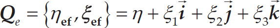
where
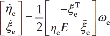
Combined with Eq. (5), the actual orientation of the end-effector when t = t f can be expressed as:

Defining {η ed , ξ ed } as the desired orientation of the end-effector, the orientation deviation of the end-effector when t = t f can be expressed as follows:

The objective function is established as:

The trajectory-planning problem proposed in Section 3 is a constrained multi-objective optimization problem, which usually involves simultaneous optimization of several competing objectives. There is no single optimal solution, but rather a set of Pareto optimal solutions. According to the Pareto dominance principle of MOP, the solutions of the optimal-trajectory-planning problem in this paper can be obtained as follows: For any two sets of joint trajectories in D, when the following relationship is satisfied,

The solution satisfying Eq. (28) is defined as a non-dominated solution of Eq. (13), which represents a set of trajectory planning that improves payload-carrying capacity as much as possible. Defining {S*} as the set of all the non-dominated solutions, the mapping of {S*} 1 on Y is an M -dimensional surface called the Pareto Front. Hence, the key to solving the multi-objective trajectory-planning problem is to achieve as many non-dominated solutions covering all features of MOP as possible. Considering the advantages of fast convergence, lower occupancy of computing resources and excellent diversity (verified by Coello [29]), the MOPSO algorithm is applied for the solution in this section.
The joint trajectories need to be parameterized before optimization. However, directly assigning the position of particles using
In order to obtain smooth and continuous trajectories of

where λkj. denotes the coefficients of the polynomial, and
Then, angular velocity and angular acceleration are computed as:


For the first type of challenge, it is assumed that

where q
k
ini
and q
k
des
denote the initial and desired angle of joint k, respectively.
Unlike in the first type,

Similarly,
In the MOPSO algorithm, g best (the best position that all the particles have had) is used as guidance to lead the evolution toward the Pareto Front. It cannot be determined immediately, but is replaced by R[h] (a value that is taken from the repository). In this paper, according to the particles' velocity formula which contains the constriction factor, the particle flight in D can be computed as follows:

where P and R denote the population and the repository, respectively; P[i] and V[i] denote the position and velocity of particle i, respectively; j = 1, 2, …, Imax is the iterations of evolutionary computations, initialization when j=0;
For the first type of challenge, the MOPSO algorithm is as follows:
Define nP as the number of particles and restrict the search range to [λmin, λmax] in each dimension of D.
Generate a random decision vector within the restrictive decision space.
Substitute the vector into Eqs. (29–31) to determine
If Eq. (16) is satisfied, store the decision vector and execute (e). Otherwise, loop to (b).
If the number of stored decision vectors equals nP, execute (f). Otherwise, loop to (b).
Locate the particles using these decision vectors as coordinates. Each particle's position in D is defined according to the value of its corresponding decision vector.
Initialize the speed of each particle using V0[i]=0.
Define n R I as the maximum allowable number of R0.
Evaluate each of the particles in P0: compute
Store the positions of particles that represent non-dominated decision vectors (according to Eq. (28)) in R0.
Generate hypercubes of Y explored so far, and locate the particles using these hypercubes as a coordinate system where the coordinate of particle i is defined according to
Initialize the best positions of the particles have had using P best 0[i]=P0[i]H stored in R0.
In Rj−1 those hypercubes containing more than one particle are assigned a fitness value equal to the result of x / N P (x > 1 and N P is the number of particles that these hypercubes contain).
Using these fitness values, roulette-wheel selection is applied to select a hypercube. Then, a random particle within the selected hypercube can be obtained. The position of this particle in decision space is taken as Rj−1[h].
Compute the speed of each particle using Eq. (34), and update the positions of the particles using
Maintain the particles' flight within the restrictive decision space: when a particle flies beyond the boundaries. Let it take the value of its corresponding boundary, and multiply its velocity by −1.
Evaluate each of the particles in P
j
by computing the objective vectors
Each selected particle which satisfies constraint conditions is defined as a new non-dominated solution. If this new solution is dominated by an individual within the external repository, then such a solution is discarded. If none of the individuals in the external repository dominates the solution, then such a solution is stored in the repository. If there are solutions in the external repository that are dominated by the new element, then such solutions are removed from the repository.
If the number of solutions in the repository has reached nR, then the adaptive grid method [29] is invoked to produce a well-distributed Pareto Front.
Define the current external repository as R j .
If P j [i] is dominated by p best j−1[i], then p best j [i] = p best j−1[i]; otherwise, p best j [i] = P j [i]; if neither is dominated by the other, then one is selected randomly.
Increment the loop counter until j = Imax.
However, for the second type of challenge, the proposed scheme cannot be used directly to solve the MOP of f1 ∼ f5. If g
i
(
Initialize the population P0 I . Define nP I as the number of particles and restrict the search range to [λmin,λmax]. Generate decision vectors and store those which satisfy Eq. (16). When the number of stored decision vectors is equal to nP I , initialize the position and velocity of each particle.
Initialize the external repository R0I. Define n R I as the maximum allowable number and store the positions of particles that represent non-dominated decision vectors in R0I (according to objective vector [f40(i), f50(i)] of the particle i). Then, initialize the best positions that the particles have had.
Adopt a similar procedure to that shown in
Initialize the population P0II. nPII equals the number of the solutions in [S I * and the search range is restricted to [λmin/ λmax]. Each particle is assigned a one-to-one position of the solution in {SI*}. Then, initialize the speed of each particle using V0II[i]=0.
Initialize the external repository R0II. Define nRII as the maximum allowable number and store the positions of particles that represent non-dominated decision vectors in R0II (according to the objective vector of the particle i:[f10(i), f20(i), f30(i), f40(i), f50(i)].) Then, initialize the best positions that the particles have had.
Adopt a similar procedure to that shown in
Simulation model
In this study, a seven-link space manipulator mounted on a base is considered. A 3D geometrical model of the manipulator is shown in Figure 2(a), and joint frames according to the DH method are shown in Figure 2(b). Relative parameters are listed in Table 1 and Table 2. d4 = 0.52m, d7 = d1 = 1.2m, d6 = d5 = d3 = d2 = 0.53m, a5 = a4 =5.8m. Pose of Σ8 is [−0.2m, 0m, 2m, 0°, 0°, 0°] with respect to Σ b , I zx = −4kg.m2.

7-DOF free-floating space manipulator
Dynamics parameters of 7-DOF space manipulator

D-H parameters of 7-DOF space manipulator

Simulations are performed to find the optimal trajectory of the 7-DOF FFSM in the two cases mentioned in Section 3.1. Fn both cases, the initial pose of the base is zero (t0=0); the total time of planning is t
f
= 100s; the upper and lower limits of joint it k(k = 7, 6, …, 1) are q
k
min = −270° and q
k
max 270°, respectively; maximum absolute linear and angular velocity of the end-effector are limited as
Case I: attaining the desired joint angles when carrying a payload.
For this case, the initial and desired angles of the joints are set as
Relevant kinematics and dynamics results using extreme solutions and trapezoidal-velocity planning

Relevant kinematics and dynamics results using extreme solutions and trapezoidal-velocity planning
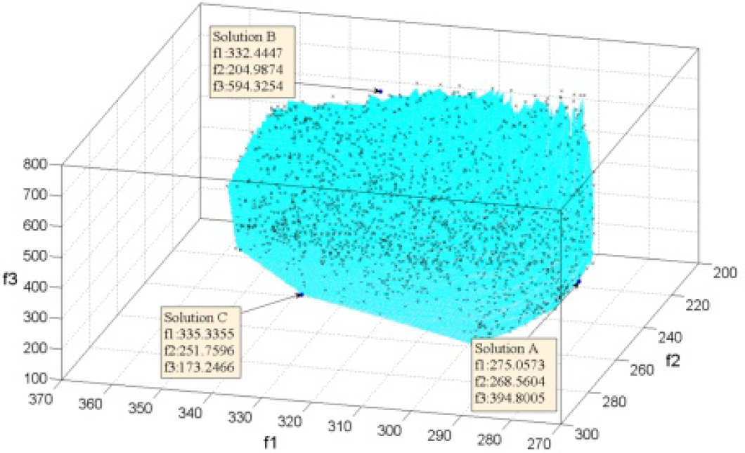
Non-dominated solution set of Case I in objective space

Optimal values of objective functions during evolution
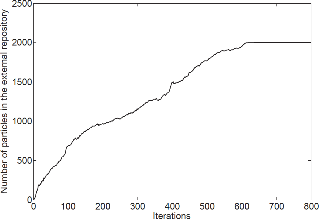
Number of particles in the repository during evolution
Solutions A, B and C marked on Figure 3 are the extreme non-dominated solutions, which correspond to the minimum value of f1, f2 and f3, respectively. Given the same parameter as Case I, contrastive simulations are performed where joint velocities are determined by conventional trapezoidal-velocity profile (mark as solution T) [30] (acceleration and deceleration time are both set as 30 seconds). The results listed in Table 3 are obtained by computing kinematics according to the four sets of joint trajectories. Although the motions of the joints, the base and the end-effector are different in these four cases, the manipulator can eventually reach the same state (configuration), while linear and angular velocities of the end-effector do not exceed the limits.
As shown in Table 3, λ A , λ B and λ T do not dominate each other, while λ C ≻ λ T . Solution A works best minimizing the driving torque of joints (f1 A reduced to 56.82% of f1 A ) and solution B works best minimizing the disturbance of the base (f2 B reduced to 75.65% of f2 T , but we see a significant increase of f3 for both solutions (f3 A = 188.53% f3 T , f3 B = 282.86% f3 T ). The decline of the other two objective functions occurs when minimizing the total energy of the whole system, in accordance with the typical characteristics of conflicts in achieving MOP goals [25].
In order to illustrate the effect of the proposed algorithm in improving load-carrying capacity, a non-dominated solution (marked as D) which dominates solution T is selected.
Case II: carrying a payload to the required pose.
For this case,
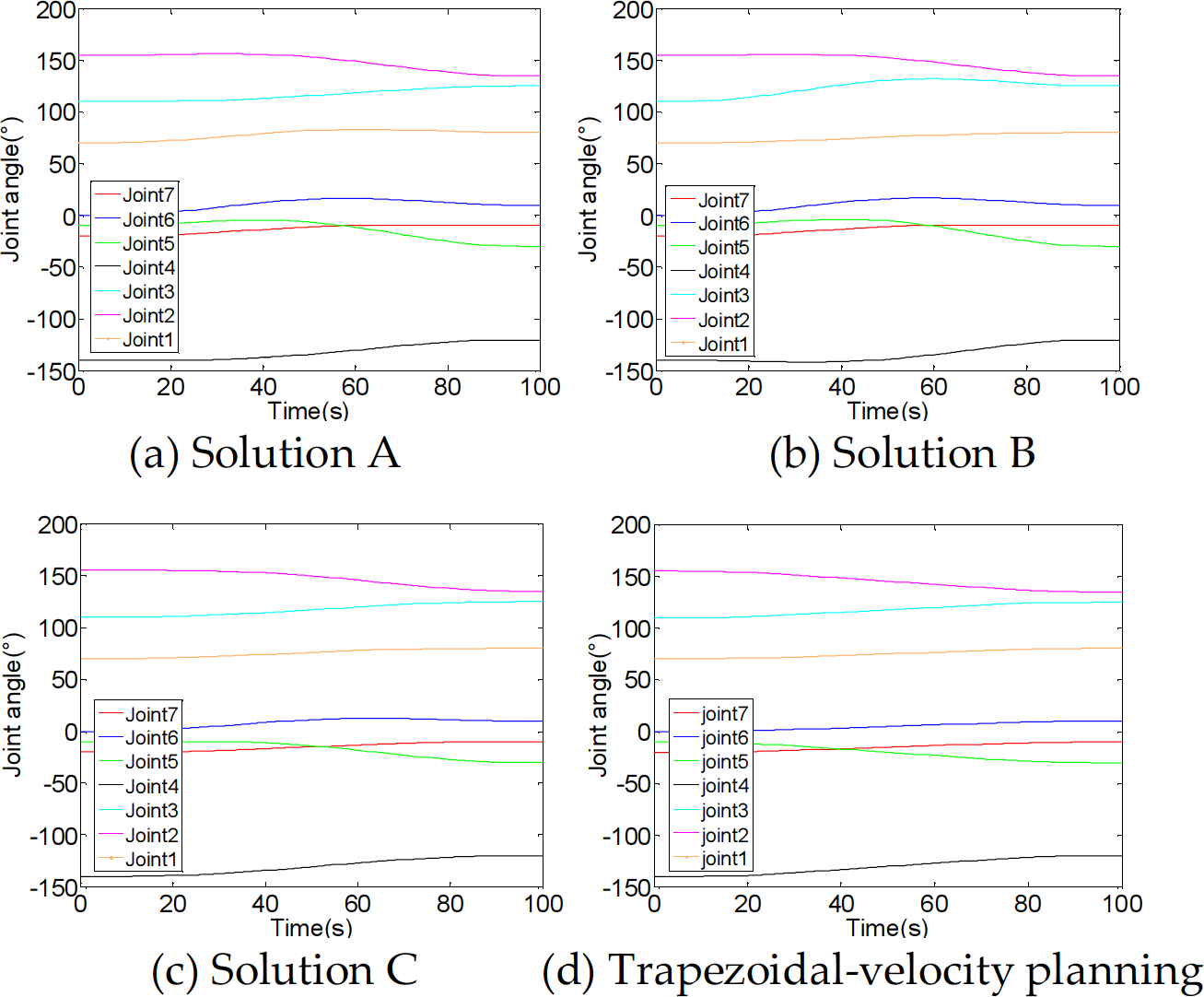
Joint trajectories using the mentioned three extreme solutions and trapezoidal-velocity planning

Joint torques and disturbance forces/torques of the base using solution D and trapezoidal-velocity planning
ETS-MARSE Denavit-Hartenberg modified parameters

The best and worst values of f1 ∼ f5 are listed in Table 4. Compared with the corresponding values of rectilinear planning, f1 ∼ f3of all the solutions in {SII*} are dominated on the premise of satisfying Eqs. (15–17), which demonstrates that maximum payload trajectory can be obtained by selecting an appropriate solution from the obtained non-dominated solution set. We define solution E as the extreme solution which minimizes f4 best.
In this paper, a MOPSO-algorithm-based scheme is developed to find the optimal joint trajectories of FFSM carrying a heavy payload. In the proposed scheme, maximization of load-carrying capacity and motion requirements of the manipulator can be achieved at the same time. Especially for the point-to-point motion in Cartesian space, a novel two-stage method is proposed to solve the optimization problem considering five objectives. The constraints are met with two measures: (i) decision vectors are specified using sinusoidal polynomial functions; (ii) solutions which do not satisfy the constraints are eliminated. Meanwhile, for the purpose of reducing computational complexity, the SOA method is adopted to compute inverse dynamics. The effectiveness of this scheme in improving load-carrying capacity is verified by simulations. It is worth noting that it is convenient for decision-makers to choose the appropriate solutions (each non-dominated solution in objective space has definite physical meanings). This kind of convenience provides the feasibility of the proposed algorithm in practical engineering. Additionally, the trajectory-planning scheme proposed in this study applies to only point-to-point motion. As another kind of typical on-orbit tasks for FFSM, trajectory tracking of the end-effector in task space exhibits significantly different characteristics and requirements. Corresponding motion-planning strategies need to be considered in future work.
Footnotes
Acknowledgements
This project is supported by the National Natural Science Foundation of China (61175080), the National Key Basic Research Programme of China (2013CB733005) and the Specialized Research Fund for the Doctoral Programme of Higher Education (20130005110009).