Subsection Evolution in GA for Trajectory Planning of a Space Manipulator

Abstract

Abstract A free-floating space manipulator has outstanding advantages and wide application prospects compared with other categories. This paper discusses the concepts and categories of space robots and introduces the current trajectory-planning algorithm for a space robot and its ground simulation system in the main countries of the world. This paper also constructs a system model for the space manipulator system and gives the kinematic equation of such a manipulator system. A dynamic equation of the manipulator's joints is also developed by using Lagrange equations. Continuous Cartesian trajectory planning is also studied in this paper based on differential kinematical equations and momentum conservation equations. Finally, this paper presents the subsection evolution algorithm in GA to realize the trajectory tracking of a free-floating space manipulator and a simulation about the free floating space manipulator and its corresponding analyses are given.

1. Introduction

Space has attracted special interest as a new application field of robotics. The space robot system, composed by a satellite and a manipulator attached to the spacecraft, is widely applied in complicated and dangerous space missions such as the capture and on-orbit services of a space target. In free-flying mode, by using the limited chemical fuel, the thruster jets of the spacecraft can compensate for the disturbance to the spacecraft caused by the movement of the manipulator. In order to conserve the precious fuel carried by the spacecraft, the thruster jets of the spacecraft should be turned off, thus the spacecraft is uncontrolled. Such a system is called an free-floating space manipulator(FFSM) system and the dynamic coupling effect between the manipulator and the spacecraft caused by the unfixed spacecraft attitude of the FFSM system is inevitable, so FFSM motions induce the disturbances to the spacecraft attitude ^[1].

A well-known space robot, the Shuttle Remote Manipulator System (SRMS or “Canadarm”) ^[2], was operated to assist the capture and berth of the satellite from the shuttle by the astronaut. NASA missions STS-61, STS-82 and STS-103 repaired the Hubble Space Telescope using astronauts with the help of SRMS. Engineering Test Satellite VII (ETS-VII) from NASDA, Japan demonstrated that the space manipulator could capture a cooperative satellite whose attitude is stabilized during the demonstration via teleoperation from the ground-base control station ^{[3, 4]}. The space robotic technologies mentioned above demonstrated the usefulness of a space robot for space service. The space manipulator is a complex flexible system, the forward and inverse kinematics equations of the manipulator involve a large number of transcendental functions such as cosine, sine, inverse tangent and square root. In conventional methods, transcendental functions are calculated by the Taylor series expansion or LUT (Look-up Table). However, the above two approaches are not attractive solutions to the real-time control of the manipulator and the accuracy of the end effector [5,6].

Many researchers have focused on kinematics, the motion-planning problems of the space manipulator systems. Papadopoulos and Tortopidis presented a path planning methodology in joint space for the planar FFSM. The method is based on mapping the non-holonomic constraint to a space where it can be satisfied trivially ^[7–9]. The reachable workspace of the FFSM with zero-disturbance spacecraft attitude is analysed and discussed in detail in [10].

The dynamic reaction forces and moments due to the manipulator motion will disturb the space base, especially when the space robot is in a free-floating situation. The longer the motion time of the space manipulator is, the greater the disturbance to the base will be. Panfeng Huang and Jie Yan presented an interval algorithm for tracking trajectory of a space manipulator for capturing an uncontrolled spinning satellite, and handled the difficulties as the feasible motion realization in joint space ^[11]. Time-optimal manipulator control strategy of a free-floating space robot is presented. The optimization procedure by Ma and Watanabe ^[12] was applied to solve the simplified optimization problem. A time-optimal control strategy of a free-floating space robot was discussed considering an arbitrary prescribed path for the manipulator hand and the dynamic constraints on reaction torque by Tomohisa Oki and Hiroki Nakanishi. The strategy was verified by numerical simulation with a free-floating space robot model equipped with a seven-DOF (degrees-of-freedom) manipulator and a system of three reaction wheels ^[13]. In [14], a manipulator path planning method for a space robot is discussed considering the limitations on the torque of reaction wheels and the manipulator path is determined by using an optimization technique.

This paper is organized as follow. Section 2 presents a model for the space manipulator system and gives the kinematic equation of such a manipulator system. A dynamic equation is also developed by using Lagrange equations. In Section 3, the procedure of the trajectory-planning algorithm in Cartesian space is explained. Also, the approach of GA developed by Panfeng Huang and Jie Yan et al. is demonstrated. In addition, the subsection evolution of GA for trajectory planning of FFSM is presented in detail. In Section 4, the simulation is shown compared to the desired trajectory. The final section summarizes the whole paper and gives some conclusions.

2. Kinematic Model, Dynamics Model And Motion Equation

A. Kinematic Model of Space Robot

In this paper, the authors assume a simple model of a space robot system, which is composed of a space base and a robotic manipulator arm mounted on the space base.

The space manipulator is installed on the space platform to fetch parts for astronauts, catch assemblies and so on. Fig. 1. depicts the structure and coordinates of the manipulator. This space manipulator is mainly composed of six modular rotary joints, one gripper and one vision camera, which is installed on the gripper. The central controller is placed on the space platform to perform kinematic control.

Figure 1.

D-H coordinates of the space manipulator

In this section, we select a manipulator with six degrees-of-freedom as our studied object.

A six-DOF space manipulator mounted on a spacecraft is used to demonstrate the analytical results. The six joints are all revolute joints. The structure and coordinate system of the space manipulator are shown in Fig. 1. The D-H parameters of the space manipulator are listed in Tab. 1.

Table 1.

D-H Parameters of the Manipulator

Joint i	ai−1	α i−1	di	θ i
1	0	0	0	θ1(0)
2	0	90°	l1	θ2(0)
3	l2	90°	0	θ3(90°)
4	l3	−90°	0	θ4(−90°)
5	0	0	l4	θ5(0)
6	l5	90°	0	θ6(90°)

The camera on the gripper gets the pose and position of the target and forms the homogeneous transform matrix ${}_{\mathrm{G}}^{\mathrm{T}}\mathrm{T}$ defined in gripper coordinate.

${\hspace{0.17em}}_{\mathrm{G}}^{\mathrm{T}}\mathrm{T}=\left[\begin{array}{cccc}{\hspace{0.17em}}^{\mathrm{T}}{\mathrm{n}}_{\mathrm{x}}& {\mathrm{o}}_{\mathrm{x}}& {\mathrm{a}}_{\mathrm{x}}& {\mathrm{p}}_{\mathrm{x}}\\ {\hspace{0.17em}}^{\mathrm{T}}{\mathrm{n}}_{\mathrm{y}}& {\mathrm{o}}_{\mathrm{y}}& {\mathrm{a}}_{\mathrm{y}}& {\mathrm{p}}_{\mathrm{y}}\\ {\hspace{0.17em}}^{\mathrm{T}}{\mathrm{n}}_{\mathrm{z}}& {\mathrm{o}}_{\mathrm{z}}& {\mathrm{a}}_{\mathrm{z}}& {\mathrm{p}}_{\mathrm{z}}\\ 0& 0& 0& 1\end{array}\right]=\left(\begin{array}{c}\begin{array}{cccc}{\mathrm{T}}_{\mathrm{n}}& {\mathrm{T}}_{\mathrm{o}}& {\mathrm{T}}_{\mathrm{a}}& {\mathrm{T}}_{\mathrm{p}}\end{array}\\ \begin{array}{cccc}0\hspace{0.17em}\hspace{0.17em}& 0& \hspace{0.17em}\hspace{0.17em}0& \hspace{0.17em}\hspace{0.17em}1\end{array}\end{array}\right)$

(1)

In order to plan the desired set points of the Cartesian coordinate trajectory for the gripper to catch the target, ${}_{\mathrm{G}}^{\mathrm{T}}\mathrm{T}$ needs to be transformed into ${}_{\mathrm{G}}^0\mathrm{T}$ and defined in the base coordinate. According to the Denavit-Hartenberg method, the transformation can be expressed in the chain product of six successive homogeneous matrices of ${}_{\mathrm{i}}^{\mathrm{i}-1}\mathrm{T}$ . ${}_{\mathrm{i}}^{\mathrm{i}-1}\mathrm{T}$ is the homogeneous transformation matrix relating the i^thcoordinate frame to the (i − 1)^th coordinate frame[15, 16].

${\hspace{0.17em}}_{\mathrm{G}}^0\mathrm{T}={\hspace{0.17em}}_{\mathrm{T}}^0\mathrm{T}\times {\hspace{0.17em}}_{\mathrm{G}}^0\mathrm{T}=({\hspace{0.17em}}^0{\mathrm{T}}_1{\hspace{0.17em}}^1{\mathrm{T}}_2\cdots {\hspace{0.17em}}^5{\mathrm{T}}_6)\times {\hspace{0.17em}}_{\mathrm{G}}^0\mathrm{T}$

(2)

Equation (2) contains a large set of trigonometric functions: sin θ_i =s_i and cos θ_i =c_i. ${}_{\mathrm{T}}^0\mathrm{T}$ can be calculated by following:

${\hspace{0.17em}}_{\mathrm{T}}^0\mathrm{T}=\hspace{0.17em}\hspace{0.17em}\left[\begin{array}{cccc}{\hspace{0.17em}}^6{\mathrm{n}}_{\mathrm{x}}& {\hspace{0.17em}}^6{\mathrm{o}}_{\mathrm{x}}& {\hspace{0.17em}}^6{\mathrm{a}}_{\mathrm{x}}& {\hspace{0.17em}}^6{\mathrm{p}}_{\mathrm{x}}\\ {\hspace{0.17em}}^6{\mathrm{n}}_{\mathrm{y}}& {\hspace{0.17em}}^6{\mathrm{o}}_{\mathrm{y}}& {\hspace{0.17em}}^6{\mathrm{a}}_{\mathrm{y}}& {\hspace{0.17em}}^6{\mathrm{p}}_{\mathrm{y}}\\ {\hspace{0.17em}}^6{\mathrm{n}}_{\mathrm{z}}& {\hspace{0.17em}}^6{\mathrm{o}}_{\mathrm{z}}& {\hspace{0.17em}}^6{\mathrm{a}}_{\mathrm{z}}& {\hspace{0.17em}}^6{\mathrm{p}}_{\mathrm{z}}\\ 0& 0& 0& 1\end{array}\right]\hspace{0.17em}$

(3)

$\begin{array}{c}{}^{6}n{}_x=-c_1{s}_2{c}_3{c}_{45}{s}_6+s_1{s}_3{c}_{45}{s}_6-c_1{c}_2{s}_{45}{s}_6-c_1{s}_2{s}_3{c}_6-s_1{c}_3{c}_6\hfill \\ {}^{6}n{}_y=-s_1{s}_2{c}_3{c}_{45}{s}_6-c_1{s}_3{c}_{45}{s}_6-s_1{c}_2{s}_{45}{s}_6-c_1{s}_2{s}_3{c}_6+c_1{c}_3{c}_6\hfill \\ \hfill {}^{6}n{}_z=c_2{c}_3{c}_{45}{s}_6-s_2{s}_{45}{s}_6+c_2{s}_3{c}_6\hfill \\ {}^{6}o{}_x=-c_1{s}_2{c}_3{c}_{45}{c}_6+s_1{s}_3{c}_{45}{c}_6-c_1{c}_2{s}_{45}{c}_6+c_1{s}_2{s}_3{s}_6+s_1{c}_3{s}_6\hfill \\ {}^{6}o{}_y=-s_1{s}_2{c}_3{c}_{45}{c}_6-c_1{s}_3{c}_{45}{c}_6-s_1{c}_2{s}_{45}{c}_6+s_1{s}_2{s}_3{s}_6-c_1{c}_3{s}_6\hfill \\ \hfill {}^{6}o{}_z=c_2{c}_3{c}_{45}{c}_6-s_2{s}_{45}{c}_6-c_2{s}_3{s}_6\hfill \\ {}^{6}a{}_x=-c_1{s}_2{c}_3{s}_4{c}_5+s_1{s}_3{s}_4{c}_5+c_1{c}_2{c}_4{c}_5-c_1{s}_2{c}_3{c}_4{s}_5+s_1{s}_3{c}_4{s}_5-c_1{c}_2{s}_4{s}_5\hfill \\ =-c_1{s}_2{c}_3{s}_{45}+s_1{s}_3{s}_4{}_5+c_1{c}_2{c}_4{}_5\hfill \\ {}^{6}a{}_y=-s_1{s}_2{c}_3{s}_4{c}_5-c_1{s}_3{s}_4{c}_5+s_1{c}_2{c}_4{c}_5-s_1{s}_2{c}_3{c}_4{s}_5-c_1{s}_3{c}_4{s}_5-s_1{c}_2{s}_4{s}_5\hfill \\ =-s_1{s}_2{c}_3{s}_4{}_5-c_1{s}_3{s}_4{}_5+s_1{c}_2{c}_4{}_5\hfill \\ \hfill {}^{6}a{}_z=c_2{c}_3{s}_{45}+s_2{c}_{45}\hfill \\ \hfill {\hspace{0.17em}}^6{\mathrm{p}}_{\mathrm{x}}=(-{\mathrm{c}}_1{\mathrm{s}}_2{\mathrm{c}}_3{\mathrm{s}}_{45}+{\mathrm{s}}_1{\mathrm{s}}_3{\mathrm{s}}_{45}+{\mathrm{c}}_1{\mathrm{c}}_2{\mathrm{c}}_{45}){\mathrm{l}}_5+(-{\mathrm{c}}_1{\mathrm{s}}_2{\mathrm{c}}_3{\mathrm{s}}_4+{\mathrm{s}}_1{\mathrm{s}}_3{\mathrm{s}}_4+{\mathrm{c}}_1{\mathrm{c}}_2{\mathrm{c}}_4){\mathrm{l}}_4+{\mathrm{c}}_1{\mathrm{c}}_2{\mathrm{l}}_{23}\hfill \\ \hfill {\hspace{0.17em}}^6{\mathrm{p}}_{\mathrm{y}}=(-{\mathrm{s}}_1{\mathrm{s}}_2{\mathrm{c}}_3{\mathrm{s}}_{45}-{\mathrm{c}}_1{\mathrm{s}}_3{\mathrm{s}}_{45}+{\mathrm{s}}_1{\mathrm{c}}_2{\mathrm{c}}_{45}){\mathrm{l}}_5+(-{\mathrm{s}}_1{\mathrm{s}}_2{\mathrm{c}}_3{\mathrm{s}}_4-{\mathrm{c}}_1{\mathrm{s}}_3{\mathrm{s}}_4+{\mathrm{s}}_1{\mathrm{c}}_2{\mathrm{c}}_4){\mathrm{l}}_4+{\mathrm{s}}_1{\mathrm{c}}_2{\mathrm{l}}_{23}\hfill \\ {\hspace{0.17em}}^6{\mathrm{p}}_{\mathrm{z}}=({\mathrm{c}}_2{\mathrm{c}}_3{\mathrm{s}}_4{}_5+{\mathrm{s}}_2{\mathrm{c}}_{45}){\mathrm{l}}_5+({\mathrm{c}}_2{\mathrm{c}}_3{\mathrm{s}}_4+{\mathrm{s}}_2{\mathrm{c}}_4){\mathrm{l}}_4+{\mathrm{s}}_2{\mathrm{l}}_{23}+{\mathrm{l}}_1\hfill \end{array}$

(4)

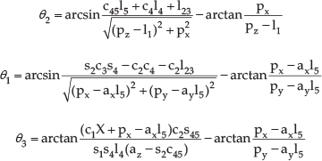
B. Inverse Kinematic for 6-DOF Manipulator

The inverse kinematics solution procedure for a six-DOF manipulator is indicated as follows:

$\cos {\theta }_4=-\frac{{\mathrm{l}}_{23}^2+{\mathrm{l}}_4^2-{\mathrm{d}}^2}{2\times {\mathrm{l}}_2{}_3\times {\mathrm{l}}_4}$

(5)

${\theta }_4=\arccos (-\frac{{\mathrm{l}}_{23}^2+{\mathrm{l}}_4^2-{\mathrm{d}}^2}{2\times {\mathrm{l}}_2{}_3\times {\mathrm{l}}_4})\hspace{0.17em}or\hspace{0.17em}-\arccos (-\frac{{\mathrm{l}}_{23}^2+{\mathrm{l}}_4^2-{\mathrm{d}}^2}{2\times {\mathrm{l}}_2{}_3\times {\mathrm{l}}_4})$

(6)

We obtain the equation from (4) as:

${({\mathrm{s}}_{45}{\mathrm{l}}_5+{\mathrm{s}}_4{\mathrm{l}}_4)}^2+{({\mathrm{c}}_{45}{\mathrm{l}}_5^{}+{\mathrm{c}}_4{\mathrm{l}}_4+{\mathrm{l}}_{23})}^2={\hspace{0.17em}}^6\mathrm{p}{}_{\mathrm{x}}^2+{\hspace{0.17em}}^6\mathrm{p}{}_{\mathrm{y}}^2+{({\hspace{0.17em}}^6{\mathrm{p}}_{\mathrm{z}}-{\mathrm{l}}_1)}^2$

(7)

Then:

${\theta }_5=\arcsin (\frac{{\mathrm{p}}_{\mathrm{x}}^2+{\mathrm{p}}_{\mathrm{y}}^2+{({\mathrm{p}}_{\mathrm{z}}-{\mathrm{l}}_1)}^2-{\mathrm{l}}_5^2-{\mathrm{s}}_4^2{\mathrm{l}}_4^2-{({\mathrm{c}}_4{\mathrm{l}}_4+{\mathrm{l}}_{23})}^2}{\mathrm{A}})-\arctan (\frac{{\mathrm{c}}_4{\mathrm{l}}_4+{\mathrm{l}}_{23}}{{\mathrm{s}}_4{\mathrm{l}}_4})-{\theta }_4$

(8)

We could also obtain the expressions as follows:

$\begin{array}{c}{\theta }_2=\arcsin \frac{{\mathrm{c}}_{45}{\mathrm{l}}_5+{\mathrm{c}}_4{\mathrm{l}}_4+{\mathrm{l}}_{23}}{\sqrt{{({\mathrm{p}}_{\mathrm{z}}-{\mathrm{l}}_1)}^2+{\mathrm{p}}_{\mathrm{x}}^2}}-\arctan \frac{{\mathrm{p}}_{\mathrm{x}}}{{\mathrm{p}}_{\mathrm{z}}-{\mathrm{l}}_1}\\ {\theta }_1=\arcsin \frac{{\mathrm{s}}_2{\mathrm{c}}_3{\mathrm{s}}_4-{\mathrm{c}}_2{\mathrm{c}}_4-{\mathrm{c}}_2{\mathrm{l}}_{23}}{\sqrt{{({\mathrm{p}}_{\mathrm{x}}-{\mathrm{a}}_{\mathrm{x}}{\mathrm{l}}_5)}^2+{({\mathrm{p}}_{\mathrm{y}}-{\mathrm{a}}_{\mathrm{y}}{\mathrm{l}}_5)}^2}}-\arctan \frac{{\mathrm{p}}_{\mathrm{x}}-{\mathrm{a}}_{\mathrm{x}}{\mathrm{l}}_5}{{\mathrm{p}}_{\mathrm{y}}-{\mathrm{a}}_{\mathrm{y}}{\mathrm{l}}_5}\\ {\theta }_3=\arctan \frac{({\mathrm{c}}_1\mathrm{X}+{\mathrm{p}}_{\mathrm{x}}-{\mathrm{a}}_{\mathrm{x}}{\mathrm{l}}_5){\mathrm{c}}_2{\mathrm{s}}_{45}}{{\mathrm{s}}_1{\mathrm{s}}_4{\mathrm{l}}_4({\mathrm{a}}_{\mathrm{z}}-{\mathrm{s}}_2{\mathrm{c}}_{45})}-\arctan \frac{{\mathrm{p}}_{\mathrm{x}}-{\mathrm{a}}_{\mathrm{x}}{\mathrm{l}}_5}{{\mathrm{p}}_{\mathrm{y}}-{\mathrm{a}}_{\mathrm{y}}{\mathrm{l}}_5}\end{array}$

C. Dynamics Model of Space Robot

Some important research achievements in space robot dynamics and control were collected by Xu and Kanade ^[17].

As shown in Fig. 3., the dynamics model assumed can be treated as a set of n + 1 rigid bodies connected with n joints that form a tree configuration, each joint numbered in a series of 1 to n. Two coordinate systems are defined. One is the inertial coordinate system Σ_i in the orbit, the other is the base coordinate system Σ₀ attached on the base body with its origin at the centroid of the base. All vectors in this paper are expressed in terms of coordinate Σ_i. Three appropriate parameters such as Roll, Pitch and Yaw are described for the attitude of the base and end-effector. Ellery ^[18] defined the notations as follows:

Figure 3.

Dynamics Model of Space Manipulator System.

Σ_i — — thei_th link frame

Σ_E — — the manipulator end-effector frame

Σ_I — — the inertial frame

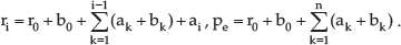
r_i — — the position of the mass centre of link i with respect to the inertial coordinates

r_G — — the position of the mass centre of the entire system with respect to the inertial coordinates

p_e — — the position of the end-effector with respect to the inertial coordinates

l_i — — the vector from joint i to joint i + 1

a_i — — the vector from joint i to the mass centre of link i

b_i — — the vector from the mass centre of link i to joint i + 1

m_i — — the mass of each rigid link i

m_T — — the total mass of the system

I_i — — the inertia matrix of link i with respect to the mass centre

ω_i — — the angular velocity of the link i

Where i = 0,1,2⃛, n

D. Kinematic and Dynamic Equation of Space Robot

Wenfu Xu and Yu Liu et al. have collected some important research on kinematic equations ^[22]. r_i and p_e are defined as the position vectors pointing toward the centre of the i _th link with respect to coordinates Σ_I and Σ₀ respectively and let r_i be the position vector pointing toward the centre of the space base with respect to inertial coordinates Σ_I. Let v_i and ω_i be linear and angular velocities of the i _th link with respect to Σ_I and let v_e and ω _e be that with respect to Σ₀, where

${\mathrm{r}}_{\mathrm{i}}={\mathrm{r}}_0+{\mathrm{b}}_0+{\displaystyle \sum _{\mathrm{k}=1}^{\mathrm{i}-1}({\mathrm{a}}_{\mathrm{k}}+{\mathrm{b}}_{\mathrm{k}})}+{\mathrm{a}}_{\mathrm{i}},{\mathrm{p}}_{\mathrm{e}}={\mathrm{r}}_0+{\mathrm{b}}_0+{\displaystyle \sum _{\mathrm{k}=1}^{\mathrm{n}}({\mathrm{a}}_{\mathrm{k}}+{\mathrm{b}}_{\mathrm{k}})}.$

Then we can obtain:

$\left[\begin{array}{c}{\mathrm{v}}_{\mathrm{e}}\\ {\omega }_{\mathrm{e}}\end{array}\right]={\mathrm{J}}_{\mathrm{b}}\left[\begin{array}{c}{\mathrm{v}}_0\\ {\omega }_0\end{array}\right]+{\mathrm{J}}_{\mathrm{m}}\stackrel{.}{\theta }$

(4)

${\mathrm{J}}_{\mathrm{b}}=\left[\begin{array}{cc}{\mathrm{E}}_3& {\mathrm{r}}_0-{\mathrm{r}}_{\mathrm{e}}\\ 0& {\mathrm{E}}_3\end{array}\right]\in {\mathrm{R}}^{6\times 6}$ is the Jacobian matrix of the centroid of the space robotic base and ${\mathrm{J}}_{\mathrm{m}}=\left[\begin{array}{c}{\mathrm{J}}_{le}\\ {\mathrm{J}}_{Rn}\end{array}\right]\in {\mathrm{R}}^{6\times 6}$ is the Jacobian matrix of the space manipulator.

The linear and the angular momentum conservation of the space manipulator are as follows:

$\mathrm{P}={\displaystyle \sum _{\mathrm{i}=0}^{\mathrm{n}}{\mathrm{m}}_{\mathrm{i}}{\stackrel{.}{r}}_{\mathrm{i}}},\mathrm{L}={\displaystyle \sum _{\mathrm{i}=0}^{\mathrm{n}}\left({\mathrm{I}}_{\mathrm{i}}{\mathrm{w}}_{\mathrm{i}}+{\mathrm{r}}_{\mathrm{i}}\times {\mathrm{m}}_{\mathrm{i}}{\stackrel{.}{r}}_{\mathrm{i}}\right)}=0$

(5)

Then we can obtain that:

$\begin{array}{l}\mathrm{P}=\left[\begin{array}{cc}ME& \mathrm{M}{\tilde{r}}_{0\mathrm{g}}^{\mathrm{T}}\end{array}\right]\left[\begin{array}{c}{\mathrm{v}}_0\\ {\mathrm{w}}_0\end{array}\right]+{\mathrm{J}}_{Tm}\stackrel{.}{\mathrm{\Theta }}=0,\\ {\mathrm{L}}_0=\left[\begin{array}{cc}\mathrm{M}{\tilde{r}}_{0\mathrm{g}}& {\mathrm{I}}_{\mathrm{W}}\end{array}\right]\left[\begin{array}{c}{\mathrm{v}}_0\\ {\mathrm{w}}_0\end{array}\right]+{\mathrm{I}}_{\phi }\stackrel{.}{\mathrm{\Theta }}=0\end{array}$

(6)

Where $\mathrm{M}={\displaystyle \sum _{\mathrm{i}=0}^{\mathrm{n}}{\mathrm{m}}_{\mathrm{i}}}$ is total mass of the entire system. ${\mathrm{J}}_{TM}={\displaystyle \sum _{\mathrm{k}=1}^{\mathrm{n}}({\mathrm{m}}_{\mathrm{k}}{\mathrm{J}}_{Ti})}\in {\mathrm{R}}^{3\times \mathrm{n}},{\mathrm{r}}_{\mathrm{g}}=\frac{{\displaystyle \sum _{\mathrm{i}=0}^{\mathrm{n}}{\mathrm{m}}_{\mathrm{i}}\times {\mathrm{r}}_{\mathrm{i}}}}{\mathrm{n}+1}$ and we define r_og =r_g – r_o. We also define ${\mathrm{I}}_{\mathrm{w}}={\displaystyle \sum _{\mathrm{i}=1}^{\mathrm{n}}({\mathrm{I}}_{\mathrm{i}}+{\mathrm{m}}_{\mathrm{i}}{\tilde{r}}_{oi}^{\mathrm{T}}{\tilde{r}}_{oi})+{\mathrm{I}}_0}$ and ${\mathrm{I}}_{\phi }={\displaystyle \sum _{\mathrm{i}=1}^{\mathrm{n}}({\mathrm{I}}_{\mathrm{i}}{\mathrm{J}}_{ai}+{\mathrm{m}}_{\mathrm{i}}{\tilde{r}}_{oi}^{\mathrm{T}}{\mathrm{J}}_{li})}$ .

Then we can obtain the momentum conservation equations of space robotics:

$\left[\begin{array}{c}\mathrm{P}\\ {\mathrm{L}}_0\end{array}\right]={\mathrm{H}}_{\mathrm{S}}\left[\begin{array}{c}{\mathrm{v}}_0\\ {\omega }_0\end{array}\right]+{\mathrm{H}}_{\phi }\stackrel{.}{\mathrm{\Theta }}=0$

(7)

Where ${\mathrm{H}}_{\mathrm{s}}=\left[\begin{array}{cc}\mathrm{M}{\mathrm{E}}_3& \mathrm{M}{\tilde{r}}_{og}^{\mathrm{T}}\\ \mathrm{M}{\tilde{r}}_{og}& {\displaystyle \sum _{\mathrm{i}=1}^{\mathrm{n}}\left({\mathrm{I}}_{\mathrm{i}}+{\mathrm{m}}_{\mathrm{i}}{\tilde{r}}_{oi}{}^{\mathrm{T}}{\tilde{r}}_{oi}\right)}+{\mathrm{I}}_0\end{array}\right]\in {\mathrm{R}}^{6\times 6}$ and ${\mathrm{H}}_{\phi }=\left[\begin{array}{c}{\mathrm{J}}_{TM}\\ {\displaystyle \sum _{\mathrm{i}=1}^{\mathrm{n}}\left({\mathrm{I}}_{\mathrm{i}}{\mathrm{J}}_{ai}+{\mathrm{m}}_{\mathrm{i}}{\tilde{r}}_{oi}^{\mathrm{T}}{\mathrm{J}}_{li}\right)}\end{array}\right]$

Then we obtain the motion equation of the space robot:

$\left[\begin{array}{c}{\mathrm{v}}_{\mathrm{e}}\\ {\omega }_{\mathrm{e}}\end{array}\right]=-({\mathrm{J}}_{\mathrm{b}}{\mathrm{H}}_{\mathrm{s}}^{-1}{\mathrm{H}}_{\phi }+{\mathrm{J}}_{\mathrm{m}})\stackrel{.}{\mathrm{\Theta }}={\mathrm{J}}_{\mathrm{g}}({\psi }_0,\stackrel{.}{\theta },{\mathrm{m}}_{\mathrm{i}},{\mathrm{I}}_{\mathrm{i}})\stackrel{.}{\mathrm{\Theta }}$

(8)

Where J_g is the generalized Jacobian matrix of the space robot.

$\mathrm{L}=\frac{1}{2}\left[{\mathrm{v}}_0^{\mathrm{T}},{\omega }_0^{\mathrm{T}},\stackrel{.}{q}\right]\left(\begin{array}{cc}{\mathrm{H}}_{\mathrm{S}}& {\mathrm{H}}_{\phi }\\ {\mathrm{H}}_{\phi }^{\mathrm{T}}& {\mathrm{H}}_{\mathrm{m}}\end{array}\right)\left[\begin{array}{c}{\mathrm{v}}_0\\ {\omega }_0\\ \stackrel{.}{\mathrm{\Theta }}\end{array}\right]=\frac{1}{2}\left[{\mathrm{v}}_0^{\mathrm{T}},{\omega }_0^{\mathrm{T}},{\stackrel{.}{\mathrm{\Theta }}}^{\mathrm{T}}\right]\mathrm{H}\left[\begin{array}{c}{\mathrm{v}}_0\\ {\omega }_0\\ \stackrel{.}{\mathrm{\Theta }}\end{array}\right]$

(9)

Where ${\mathrm{H}}_{\mathrm{m}}={\displaystyle \sum _{\mathrm{i}=1}^{\mathrm{n}}\left({\mathrm{J}}_{ai}{}^{\mathrm{T}}•{\mathrm{I}}_{\mathrm{i}}•{\mathrm{J}}_{ai}+{\mathrm{m}}_{\mathrm{i}}{\mathrm{J}}_{ai}{}^{\mathrm{T}}•{\mathrm{J}}_{ai}\right)}$ and $\mathrm{H}=\left(\begin{array}{cc}{\mathrm{H}}_{\mathrm{S}}& {\mathrm{H}}_{\phi }\\ {\mathrm{H}}_{\phi }^{\mathrm{T}}& {\mathrm{H}}_{\mathrm{m}}\end{array}\right)\in {\mathrm{R}}^{(\mathrm{n}+6)\times (\mathrm{n}+6)}$

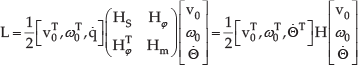
We define generalized coordinates $\mathrm{q}={\left[{\mathrm{v}}_0^{\mathrm{T}},{\omega }_0^{\mathrm{T}},{\mathrm{\Theta }}^{\mathrm{T}}\right]}^{\mathrm{T}}$ and generalized force $\tau =\left[\begin{array}{c}{\mathrm{F}}_{\mathrm{b}}\\ {\mathrm{F}}_{\mathrm{m}}\end{array}\right]+\left[\begin{array}{c}{\mathrm{J}}_{\mathrm{b}}^{\mathrm{T}}\\ {\mathrm{J}}_{\mathrm{m}}^{\mathrm{T}}\end{array}\right]{\mathrm{F}}_{\mathrm{e}}$ . F_b and F_m ∈ R6 are the forces on the base and the manipulator of the space robot, F_b is the external force on the end of manipulator. We assume that $\mathrm{C}(\mathrm{q},\stackrel{.}{q})=\left[\begin{array}{c}{\mathrm{c}}_{\mathrm{b}}\\ {\mathrm{c}}_{\mathrm{m}}\end{array}\right]$ and ${\mathrm{c}}_{\mathrm{b}},{\mathrm{c}}_{\mathrm{m}}\in {\mathrm{R}}^6$ are, respectively, nonlinear forces with respect to the motion of the base and the manipulator (Coriolis force and centripetal force).

Then we can obtain the Lagrange dynamic Equation:

$\left[\begin{array}{cc}{\mathrm{H}}_{\mathrm{S}}& {\mathrm{H}}_{\phi }\\ {\mathrm{H}}_{\phi }^{\mathrm{T}}& {\mathrm{H}}_{\mathrm{m}}\end{array}\right]\left[\begin{array}{c}{\stackrel{.}{v}}_0\\ {\stackrel{.}{\omega }}_0\\ \stackrel{..}{\mathrm{\Theta }}\end{array}\right]+\left[\begin{array}{c}{\mathrm{c}}_{\mathrm{b}}\\ {\mathrm{c}}_{\mathrm{m}}\end{array}\right]=\left[\begin{array}{c}{\mathrm{F}}_{\mathrm{b}}\\ {\mathrm{F}}_{\mathrm{m}}\end{array}\right]+\left[\begin{array}{c}{\mathrm{J}}_{\mathrm{b}}^{\mathrm{T}}\\ {\mathrm{J}}_{\mathrm{m}}^{\mathrm{T}}\end{array}\right]{\mathrm{F}}_{\mathrm{e}}$

(10)

It has been found that free-floating systems are subject to unpredictable dynamic singularities in their manipulator workspaces owing to the attitude motion of the platform at which point they become unstable ^{[19, 20]} Indeed, dynamic singularities are characteristic of free-floating systems and are functions of the mass and inertia of the composite spacecraft/manipulator system. These singular joint configurations cannot be mapped into unique points in the workspace since the generalized Jacobian is a dynamic function rather than being purely kinematic and spacecraft attitude coordinates do not map uniquely to end-effector coordinates.

The bidirectional search mapped between the original state and the final desired configuration using the generalized Jacobian to avoid excessive joint torques is used for obstacle avoidance or for reorientation of attitude. A Moore-Penrose pseudo-inverse version of the generalized Jacobian ${\mathrm{J}}_{\mathrm{g}}^{+}={\mathrm{J}}_{\mathrm{g}}^{\mathrm{T}}{({\mathrm{J}}_{\mathrm{g}}{\mathrm{J}}_{\mathrm{g}}^{\mathrm{T}})}^{-1}$ was used to overcome the dynamic singularities problem by using the redundant degrees of freedom ^[21]. It allowed changes in spacecraft attitude while keeping the generalized position of the end-effector fixed with respect to the inertial reference frame to provide greater flexibility of operation.

3. Subsection Evolution in Trajectory-Planning

A. Trajectory Planning in Cartesian Space

Trajectory planning in Cartesian space is always described as follows:

• Step 1.

Set the continuous trajectory of the manipulator end-effector in Cartesian space as p_e (t), ϕ_e (t).

Step 2.

Plan the linear velocity of the manipulator end-effector by v_e (t) = ṗ_e (t).

Step 3.

Plan the angular velocity of the manipulator end-effector by ${\mathrm{v}}_{\mathrm{e}}\left(\mathrm{t}\right)={\stackrel{.}{p}}_{\mathrm{e}}\left(\mathrm{t}\right)$ , where $\mathrm{r}=\frac{{\mathrm{e}}_0}{\left|{\mathrm{e}}_0\right|},{\mathrm{e}}_0$ is the direction deviation of the manipulator end-effector.

Step 4.

Compute the velocity of the joint on the inverse kinematics equation by the angular and linear velocity of the manipulator end-effector ${\stackrel{.}{\theta }}_{\mathrm{d}}\left(\mathrm{t}\right)={\left({\mathrm{J}}_{\mathrm{g}}\left(\mathrm{t}\right)\right)}^{-1}\left[\begin{array}{c}{\mathrm{v}}_{\mathrm{e}}\\ {\omega }_{\mathrm{e}}\end{array}\right]$ .

Where J_g⁻¹ is the inverse damping minimum variance of the generalized Jacobian matrix of the space robot. It can be presented as: ${\left({\mathrm{J}}_{\mathrm{g}}\right)}^{-1}={\left({\mathrm{J}}_{\mathrm{g}}\right)}^{\mathrm{T}}{\left[{\mathrm{J}}_{\mathrm{g}}{\left({\mathrm{J}}_{\mathrm{g}}\right)}^{-1}+{\lambda }^2\mathrm{I}\right]}^{-1}$ . Then ${\theta }_{\mathrm{d}}\left(\mathrm{t}+\mathrm{\Delta }\mathrm{t}\right)=\theta \left(\mathrm{t}\right)+{\stackrel{.}{\theta }}_{\mathrm{d}}\left(\mathrm{t}\right)\mathrm{\Delta }\mathrm{t}$ , where Δt is the joint control period and the damping factor 0 < λ ≤ 1.

Step 5.

Compute the angular velocity of the space manipulator base attitude by (7), then obtain the base attitude Φ_o by numerical integration.

Trajectory planning in Cartesian Space calculates the movement of six joint angles by an inverse generalized Jacobian matrix of the space robot and the expected trajectory of the manipulator end-effector. It has some disadvantages such as reliance on the inverse velocity kinematics equation and is influenced by the singular value of the Jacobian matrix.

B. Genetic Algorithms-Based Minimum Torque Path Planning for a Space Manipulator

In the space environment, the power supply for a space manipulator is limited because of the lower ratio of the solar array. Panfeng Huang and Jie Yan presented a minimum torque path-planning scheme for a space manipulator, which used a Genetic Algorithm (GA) to minimize the objective function. The planning procedure was performed in the joint space and with respect to all constraints, such as joint angle constraints, joint velocity constraints and torque constraints. GA was used to search for the optimal joint inter-knot parameters in order to realize the minimum-torque.

The basic optimal processes of GA are illustrated in Fig. 4. The algorithm procedure in ^[22] can optimize the trajectory using the genetic algorithm as follows:

Figure 4.

Optimization procedure using genetic algorithm

• Step 1.

  Choose the number of inter-knots m, then determine the path planning strategies for each path segment. Encode the parameters of every inter-knot using the chromosomes of GA.

• Step 2.

  Define the fitness function according to the cost function and constraints. Define GA parameters, such as population size n_p, generation number n_g, crossover probability p_c and effective gene number n_e. Let generation number n_g = 1.

• Step 3.

  Randomly generate a population of binary strings, ${\text{pop}}^{\mathrm{k}}=\mathrm{b}{\mathrm{s}}_{\mathrm{l}}^{\mathrm{k}}|\mathrm{l}=1,\dots ,{\mathrm{n}}_{\mathrm{p}}$ .

• Step 4.

  Let l = 1.

• Step 5.

  Decode each binary string bs₁^k into parameter

  ${\text{pop}}^{\mathrm{k}}=\mathrm{b}{\mathrm{s}}_{\mathrm{l}}^{\mathrm{k}}|\mathrm{l}=1,\dots ,{\mathrm{n}}_{\mathrm{p}}.$
  Use 4-4-, …,-4-5 iterative path planning strategy ^[23] to plan the path Q_ij^k with pop₁^k.

• Step 6.

  Compute the maximum joint angle, joint angular velocity, joint angular acceleration, q_ijmax^k and v_ijmax^k with respect to the path Q_ij^k.

• Step 7.

  Compute every joint torque using inverse dynamics according to the maximal position, velocity and acceleration of the joint, q_ijmax^k, v_ijmax^k.

• Step 8.

  Let l = l + 1 and return to Step 5 until l = n_p.

• Step 9.

  Summarize the absolute values of all torques from l = 1 to l = n according to fitness function. Collect the minimum fitness function value.

• Step 10.

  Let k = k + 1, generate a new population pop^k using reproduction, crossover and mutation operators. Return to Step 4 until k = n_g

• Step 11.

  Obtain the minimum fitness function value, thus, the parameters in this situation as optimal values. Get the optimum trajectory Q_ij^*.

Firstly, some inter-knots were selected to generate the trajectory segments. In each trajectory segment, a suitable polynomial is used to obtain the local trajectory. Thus, the whole trajectory is planned iteratively and its performance can be calculated according to the fitness function in which cost function and constraints are taken into account. The parameters of the inter-knots of each trajectory segment were optimized by the GAs. Meanwhile, the path is evolved into the optimum trajectory connecting initial and the final points in the joint space.

In [23], GA was used to solve the optimal trajectory planning described by the cost function with a dynamic model under initial and final conditions and constraints. The whole trajectory was divided into several trajectory segments. The path point connecting with two segments was called the knot point. The optimal algorithm was to search for the optimum parameters of each knot point, such as joint angle and joint angular velocity, then to realize minimum torque trajectory planning. The coefficients of the polynomials depended on the trajectory parameters, q_ij and v_ij if the travel time t_f of every trajectory segment was fixed ^[24]. Therefore, these parameters will be evolved by the genetic algorithm.

Figure 5.

Joint position trajectory, angular velocity, Joint angular acceleration and Joint torque versus time for 2-DOF manipulator

C. Trajectory Planning on subsection evolution using GA

In this section, the steps of the trajectory planning for FFSM is presented. Firstly, we set a continuous trajectory of end-effector and divide the whole trajectory into a variety of subsections. We call the path points as inter-knots which cut the trajectory into sections. Then we encode the parameters of every subsection and define GA parameters and also fitness function according to the kinetic energy. Then we obtain the movement, velocity and acceleration of the joints by calculating the population. The apprach could search for the optimum parameters of the subsection to realize minimum energy planning. The new algorithm procedure to optimize the trajectory using subsection evolution by a genetic algorithm is as follows:

• Step 1.

Set the continuous trajectory of the manipulator end-effector p_e(t), then set the n inflection points as the crucial segmentation points to divide the trajectory into n − 1 parts of the whole trajectory. Choose the number m − 1 to divide each subsection by inter-knots, then the number m, n of initial inter-knots can be obtained. Draw a circle with the centre at each initial inter-knot and with a radius equal to r_i. Obtain the inter-knots by proportional spacing. Encode the parameters of every subsection using chromosomes of GA and generate the initial population. The initial inter-knots, which construct different subsections, are connected to form a continuous trajectory.

Step 2.

Define fitness function according to kinetic energy.

The whole kinetic energy of the space system is already expressed:

$\mathrm{L}=\frac{1}{2}\left[{\mathrm{v}}_0^{\mathrm{T}},{\omega }_0^{\mathrm{T}},\stackrel{.}{q}\right]\left(\begin{array}{cc}{\mathrm{H}}_{\mathrm{S}}& {\mathrm{H}}_{\phi }\\ {\mathrm{H}}_{\phi }^{\mathrm{T}}& {\mathrm{H}}_{\mathrm{m}}\end{array}\right)\left[\begin{array}{c}{\mathrm{v}}_0\\ {\omega }_0\\ \stackrel{.}{\mathrm{\Theta }}\end{array}\right]=\frac{1}{2}\left[{\mathrm{v}}_0^{\mathrm{T}},{\omega }_0^{\mathrm{T}},{\stackrel{.}{\mathrm{\Theta }}}^{\mathrm{T}}\right]\mathrm{H}\left[\begin{array}{c}{\mathrm{v}}_0\\ {\omega }_0\\ \stackrel{.}{\mathrm{\Theta }}\end{array}\right]$

(9)

$\mathrm{f}(\mathrm{x})=\{\begin{array}{c}{\mathrm{C}}_{\max }-\frac{1}{2}\left[{\mathrm{v}}_0^{\mathrm{T}},{\omega }_0^{\mathrm{T}},{\stackrel{.}{\mathrm{\Theta }}}^{\mathrm{T}}\right]\mathrm{H}\left[\begin{array}{c}{\mathrm{v}}_0\\ {\omega }_0\\ \stackrel{.}{\mathrm{\Theta }}\end{array}\right]\hspace{0.17em}\hspace{0.17em}\hspace{0.17em}\hspace{0.17em}\hspace{0.17em}\hspace{0.17em}\hspace{0.17em}\hspace{0.17em}\hspace{0.17em}\hspace{0.17em}\hspace{0.17em}\hspace{0.17em}when\hspace{0.17em}\mathrm{g}(\mathrm{x})<{\mathrm{C}}_{\max }\\ \hspace{0.17em}\hspace{0.17em}\hspace{0.17em}\hspace{0.17em}\hspace{0.17em}\hspace{0.17em}\hspace{0.17em}\hspace{0.17em}\hspace{0.17em}\hspace{0.17em}\hspace{0.17em}\hspace{0.17em}\hspace{0.17em}\hspace{0.17em}\hspace{0.17em}\hspace{0.17em}\hspace{0.17em}\hspace{0.17em}\hspace{0.17em}\hspace{0.17em}\hspace{0.17em}\hspace{0.17em}\hspace{0.17em}\hspace{0.17em}0\hspace{0.17em}\hspace{0.17em}\hspace{0.17em}\hspace{0.17em}\hspace{0.17em}\hspace{0.17em}\hspace{0.17em}\hspace{0.17em}\hspace{0.17em}\hspace{0.17em}\hspace{0.17em}\hspace{0.17em}\hspace{0.17em}\hspace{0.17em}\hspace{0.17em}\hspace{0.17em}\hspace{0.17em}\hspace{0.17em}\hspace{0.17em}\hspace{0.17em}\hspace{0.17em}\hspace{0.17em}\hspace{0.17em}\hspace{0.17em}\hspace{0.17em}\hspace{0.17em}\hspace{0.17em}\hspace{0.17em}\hspace{0.17em}\hspace{0.17em}\hspace{0.17em}others\hspace{0.17em}\hspace{0.17em}\hspace{0.17em}\hspace{0.17em}\hspace{0.17em}\hspace{0.17em}\end{array}$

(11)

Where, C_max is the total energy consumed by the system.

Step 3.

Define GA parameters.

Mutation:

Every new inter-knot is generated by the circle with the centre at each initial inter-knot and with a radius equal to r_i. Every new inter-knot creates a new trajectory after every generation. The mutation rate p_m = 0.05.

Crossover:

As shown in Fig. 6., two trajectories exchange two inter-knots to create new trajectories for crossover. The crossover parameters M_c are determined by the crossover rate p_c. We set p_c = 0.4 in this paper.

Figure 6.

Mutation operator

Reproduction:

We determine the roulette wheel method, which is the base of GA ^[22] and set the reproduction rate p_r = 0.2.

Step 4. Let generation number Gen = 1

Step 5. Obtain the movement, velocity and acceleration of the joints by calculating the population. Solve the generalized Jacobian matrix of the space robot J_g by the performance of the joints and the base to the inertial coordinate system. Calculate the velocity of every joint and the base by the inverse kinematics equation of velocity. Obtain the fitness function value.

Figure 7.

Crossover operator

Step 6. Let Gen = Gen+ 1

Step 7. Generate a new population using reproduction, crossover and mutation operators. Go to Step 4.

Step 8. Obtain the minimum fitness function value.

Calculate the error ζ_e of the end of the space manipulator to judge whether or not it's within the allowable error ζ. If ζ_e > ζ, Go to Step 4. If ζ_e ≤ ζ, the parameters in this situation are optimal values. Obtain the optimum trajectory.

4. Simulation

The detailed derivation of dynamic equations of space robots can be obtained from Section 2. The parameters of the space robot are shown in Table 2. For a real space robot system, the joint angle, angular velocity, acceleration and torque of the manipulator should have constraint values. We can define the constraint conditions of the model of a space robot as follows:

Table 2.

Parameters of Space Robot System

				Ikg · m2)
Link	li (m)	mi(kg)
			Ixx	Iyy	Izz
Sat	0.2	400	30	25	30
Link1	0.3	5	0.105	0.105	0.05
Link2	0.6	5	0.25	0.25	0.075
Link3	0.8	6	0.4	0.3	0.15
Link4	0.3	4	0.15	0.15	0.1
Link5	0.3	3	0.1	0.1	0.05
Link6	0.1	2	0.05	0.05	0.02

$\begin{array}{l}{\mathrm{v}}_{\mathrm{i}\max }=3rad/\mathrm{s},\mathrm{i}=1,2,\dots ,6\\ {\mathrm{a}}_{\mathrm{i}\max }=5rad/{\mathrm{s}}^2,\mathrm{i}=1,2,\dots ,6\end{array}$

According to the simulation result, Fig.8. shows the trajectory of the manipulator end-effector. The plot shows that it starts from the initial position at t = 0 seconds and reaches the final position at t = 40 seconds. It also shows the linear velocity and acceleration of the manipulator end-effector.

Figure 8.

Trajectory of end-effector

The goal of the simulation is to verify the performance of GA optimization.

As shown in Fig. 8, the planned path is smoother and more applicable for the control of the manipulator. The structure of the algorithm is more flexible for solve the general problems in these kinds of algorithms using inter-knots if introducing the other parameters such as the corner points by generating inter-knots. The error between the actual trajectory and the desired trajectory can be kept in an allowed range by introducing the error parameter into the algorithm. The number of inter-knots is chosen manually before by research. The approach in this paper generates the inter-knots in a particular way to reduce time by selecting the points.(In Fig.8, the unit of the Y axis is cm.)

Figure 9.

The simulation of space manipulator

It is necessary to study how many inter-knots are optimal for optimization. Obviously, the more inter-knots, the more complicated problem, which certainly costs more time for computation. Thus, choosing the smallest number of inter-knots is optimal. However, optimal precision may increase when adding the number of inter-knots. More inter-knots will be verified in the future work.

5. Conclusion

In this paper, a new subsection evolution algorithm for trajectory planning is developed. The method is based on genetic algorithms, which can search most satisfactory parameters of subsections to generate the optimal motion path. The optimal path obtained is fit for high velocity and high precision dynamic control.

6. Acknowledgement

This work is supported by the Program for Changjiang Scholars and Innovative Research Team in University(No.IRT1109), the Program for Liaoning Science and Technology Research in University (No.LS2010008), the Program for Liaoning Innovative Research Team in University(No.LT2011018), Natural Science Foundation of Liaoning Province (201102008), the Program for Liaoning Key Lab of Intelligent Information Processing and Network Technology in University and by “Liaoning BaiQianWan Talents Program(2010921010, 2011921009)”.