Backstepping Based Trajectory Tracking Control of a Four Wheeled Mobile Robot

Abstract

For a four wheeled mobile robot a trajectory tracking concept is developed based on its kinematics. A trajectory is a time–indexed path in the plane consisting of position and orientation. The mobile robot is modeled as a non holonomic system subject to pure rolling, no slip constraints. To facilitate the controller design the kinematic equation can be converted into chained form using some change of co-ordinates. From the kinematic model of the robot a backstepping based tracking controller is derived. Simulation results demonstrate such trajectory tracking strategy for the kinematics indeed gives rise to an effective methodology to follow the desired trajectory asymptotically.

1. Introduction

A mobile robot is one of the well known system with nonholonomic constraints and there are many works on its tracking control. Their objective are mostly the kinematics model. For non holonomic systems such as mobile robots their kinematics constraints make time derivative of some configuration variables nonintegrable (Xiaoping, Y. & Yamamoto, Y., 1996). Due to the appearance of the nonholonomic constraints the motion planning and the tracking control of mobile robots are difficult to be managed. In the phase of motion planning (Wilson, D.E., and Luciano, E.C., 2002) a suitable trajectory is designed to connect the initial posture (i.e the position and orientation of the robot) and the final one such that no collisions with obstacles would occur and kinematics constraints are satisfied. Once the feasible path is obtained the navigation and control process enters the tracking phase. In this paper we restrict our attention to the kinematics of the nonholonomic systems such that every path can be followed efficiently. In (Kanayama, Y., kimura, Y., Miyazaki, F. & Noguchi, T., 1990) a linearization based tracking control scheme was introduced for a two degree of freedom mobile robot. A similar idea was independently examined by Walsh et al. in (Walsh, G., Tilbury, D., Sastry, S., Murray, R. & Laumond, J.P., 1994). The idea of input-output linearization was further explored by (Oelen, W. & Amerongen, J., 1994) for a two degree of freedom mobile robot. All these papers solve the local tracking problem for some classes of nonholonomic systems. The class of nonholonomic system in chained form was introduced by (Murray, R. M., & Sastry, S.S., 1993) and has been studied as a bench mark example by several authors. It is well known that many mechanical system with nonholonomic constraints can be locally or globally, converted to chained form under coordinate change and state feedback. Interesting examples of such mechanical systems include tricycle-type mobile robots, cars towing several trailers, the knife edge (Murray, R. M., & Sastry, S.S., 1993), (Kolmanovsky, I. & McClamroch, N. H., 1995). Trajectory planning algorithm for a four-wheel-steering (4WS) vehicle based on vehicle kinematics was introduced by (Danwei, W. & Feng, Q., 2001). Trajectory tracking control of tri-wheeled mobile robots in skew chained form system was introduced by (Tsai, P.S., Wang, L.S., & Chang, F.R., 2006).

In this paper we develop the kinematic model of a four wheel nonholonomic mobile robot subject to pure rolling and no side slipping condition and we propose a systematic control design procedure for chained form obtained from the kinematic model. The stepwise control design procedure used in this paper is based on the backstepping approach. The problem to be solved here is the tracking of a desired reference trajectory for a four wheeled mobile robot moving on a horizontal plane and simulation results were presented to illustrate the approach.

2. Model of the mobile robot

2.1 Introduction

In this section kinematic model of the four wheel nonholonomic mobile robot is presented. In order to simplify the mathematical model of the four wheel nonholonomic wheeled mobile robot we assume that

The wheeled mobile robot is built from rigid mechanism.

There is zero or one steering link per wheel.

All steering axes are perpendicular to the surface of motion.

The surface is a smooth plane.

No slip occurs between the wheel and the floor.

2.2 Instantaneous centre of rotation (ICR)

It is an imaginary point around which a rigid body appears to be rotating momentarily (for an instant) when the body is rotating and translating. For a four wheel mobile robot the instantaneous centre of rotation is the cross point of all axes of the wheels. Its importance lies in the fact that wheel axes must intersect at a point if there is no slipping.

2.3 Kinematic model of the four wheel mobile robot

In this section the kinematic model is developed. A wheeled mobile robot is a wheeled vehicle which is capable of an autonomous motion (without external human driver) because it is equipped, for its motion, with motors that are driven by an embarked computer. The four wheel mobile robot considered in this paper is shown in figure 1, its front wheels are steering wheels, and its rear wheels are driving wheels. The distance between the front wheel axle and platform centre of gravity is c and distance between the rear wheel axle and platform centre of gravity is d and 2b is the wheel span. The trajectory planning will be done for the platform centre of gravity. Let the generalized co-ordinates be q = [x₀, y₀, φ₀, φ]^T, where (x, y) are the cartesian coordinates of the centre of gravity of the mobile platform with respect to co-ordinate frame {U}. The four wheels are located at p₁, p₂, p₃ and p₄ on the mobile platform respectively. p_c is the centre of the mobile platform. Six co-ordinate frames are defined for describing position and orientation of the mobile robot.{1} is the frame fixed on wheel 1. x₁ - axis is choosen to be along the horizontal radial direction and y₁ axis in the lateral direction. Likewise {2},{3} and {4} are the frame defined for the wheel 2, 3 and 4 respectively.{0} is the frame defined at point p_c. The orientation of the vehicle body is characterized by φ₀ which is the angle from x_U to x₀. f₁ and f₂ are the front two steering angle and φ is the angle at which the whole platform changes the orientation due to steering angles φ₁ and φ₂ of the front two steering wheels. With these notations we establish homogenious transformations describing one frame relative to another. ${\hspace{0.17em}}_b^{a}T$ denotes the homogenious transformation of frame {b} relative to frame {a}. Because the motion of the mobile robot is restricted to 2-dimentional plane homogenious transformation matrices are 3 × 3 rather than 4 × 4 and are given by

$$\begin{array}{l}{\hspace{0.17em}}_0^{U}T=\left[\begin{array}{ccc}\cos {\varphi }_0& -\sin {\varphi }_0& x_0\\ \sin {\varphi }_0& \cos {\varphi }_0& y_0\\ 0& 0& 1\end{array}\right],\\ {}_1^{0}T=\left[\begin{array}{ccc}\cos {\varphi }_1& -\sin {\varphi }_1& c\\ \sin {\varphi }_1& \cos {\varphi }_1& b\\ 0& 0& 1\end{array}\right]\\ {\hspace{0.17em}}_3^{0}T=\left[\begin{array}{ccc}\cos {\varphi }_2& -\sin {\varphi }_2& c\\ \sin {\varphi }_2& \cos {\varphi }_2& -b\\ 0& 0& 1\end{array}\right]\\ {\hspace{0.17em}}_3^{0}T=\left[\begin{array}{ccc}1& 0& -d\\ 0& 1& b\\ 0& 0& 1\end{array}\right]{,}_4^{0}T=\left[\begin{array}{ccc}1& 0& -d\\ 0& 1& -b\\ 0& 0& 1\end{array}\right]\end{array}$$

Fig. 1:

Four wheel mobile robot and co-ordinate frame

2.4 Velocities

With the help of homogenious transformation given above the velocities of point p₁, p₂, p₃ and p₄ can be easily computed.

The homogenious position vector of point p₁ in frame {0} is

$${}^0{P}_1=\left[\begin{array}{c}c\\ b\\ 1\end{array}\right]$$

The same point is represented in frame {U} by

$$\begin{array}{l}{}^U{P}_1{=}_0^{U}T{}^0{P}_1\\ =\left[\begin{array}{c}c\cos {\varphi }_0-b\sin {\varphi }_0+x_0\\ c\sin {\varphi }_0-b\cos {\varphi }_0+y_0\\ 1\end{array}\right]\end{array}$$

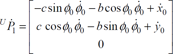
The velocity of point p₁ relative to frame {U} expressed in frame {U} is then

$${}^U{\dot{P}}_1=\left[\begin{array}{c}-c\sin {\varphi }_0{\dot{\varphi }}_0-b\cos {\varphi }_0{\dot{\varphi }}_0+{\dot{x}}_0\\ c\cos {\varphi }_0{\dot{\varphi }}_0-b\sin {\varphi }_0{\dot{\varphi }}_0+{\dot{y}}_0\\ 0\end{array}\right]$$

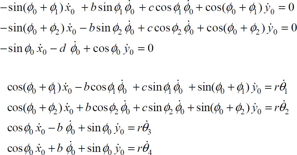
In order to derive the nonholonomic constraint equation of wheel 1. The velocity of point p₁ relative to frame {U} is expressed in frame {1} is

$$\begin{array}{l}{}^1{\dot{P}}_1={(}^U{T}_1)-1{}^U{\dot{P}}_1\\ ={\left\{\left[\begin{array}{ccc}\cos {\varphi }_0& -\sin {\varphi }_0& x_0\\ \sin {\varphi }_0& \cos {\varphi }_0& y_0\\ 0& 0& 1\end{array}\right]\cdot \left[\begin{array}{ccc}\cos {\varphi }_1& -\sin {\varphi }_1& c\\ \sin {\varphi }_1& \cos {\varphi }_1& b\\ 0& 0& 1\end{array}\right]\right\}}^{-1}\cdot {}^U{\dot{P}}_1\\ =\left[\begin{array}{c}\cos ({\varphi }_0+{\varphi }_1){\dot{x}}_0-b\cos {\varphi }_1{\dot{\varphi }}_0+c\sin {\varphi }_1{\dot{\varphi }}_0+\sin ({\varphi }_0+{\varphi }_1){\dot{y}}_0\\ -\sin ({\varphi }_0+{\varphi }_1){\dot{x}}_0+b\sin {\varphi }_1{\dot{\varphi }}_0+c\cos {\varphi }_1{\dot{\varphi }}_0+\cos ({\varphi }_0+{\varphi }_1){\dot{y}}_0\\ 0\end{array}\right]\end{array}$$

Similarly the velocity of point 2, 3, 4 relative to frame {U} expressed in frame {2}, {3} and {4} as follows

$$\begin{array}{l}{}^2{\dot{P}}_2=\left[\begin{array}{c}\cos ({\varphi }_0+{\varphi }_2){\dot{x}}_0+b\cos {\varphi }_2{\dot{\varphi }}_0+c\sin {\varphi }_2{\dot{\varphi }}_0+\sin ({\varphi }_0+{\varphi }_2){\dot{y}}_0\\ -\sin ({\varphi }_0+{\varphi }_2){\dot{x}}_0+b\sin {\varphi }_2{\dot{\varphi }}_0+c\cos {\varphi }_2{\dot{\varphi }}_0+\cos ({\varphi }_0+{\varphi }_2){\dot{y}}_0\\ 0\end{array}\right]\\ {}^3{\dot{P}}_3=\left[\begin{array}{c}\cos {\varphi }_0{\dot{x}}_0-b{\dot{\varphi }}_0+\sin {\varphi }_0{\dot{y}}_0\\ -\sin {\varphi }_0{\dot{x}}_0-d{\dot{\varphi }}_0+\cos {\varphi }_0{\dot{y}}_0\\ 0\end{array}\right]\\ {}^4{\dot{P}}_4=\left[\begin{array}{c}\cos {\varphi }_0{\dot{x}}_0-b{\dot{\varphi }}_0+\sin {\varphi }_0{\dot{y}}_0\\ -\sin {\varphi }_0{\dot{x}}_0-d{\dot{\varphi }}_0+\cos {\varphi }_0{\dot{y}}_0\\ 0\end{array}\right]\end{array}$$

2.5 Constraint equations

To develop the kinematic model of the wheeled mobile robot, the ith wheel is considered as rotating with angular velocity ${\dot{\theta }}_i$ where ${\dot{\theta }}_i$ , i = 1, 2, 3, 4. denotes the angular velocities for each wheel. For simplicity the thickness of the wheel is neglected and is assumed to touch the plane at P _i as illustrated in fig.2. Further it is assumed that during the motion the plane of each wheel remain vertical and the wheel rotates around its (horizontal) axle whose orientation with respect to the frame can be fixed or varying. The first four constraints in which two constraint are identical are due to no slip condition i.e pure rolling and the other four constraints obtained from the condition that the wheels can not move in the lateral direction (i.e y-component of ${\hspace{0.17em}}^1{\dot{P}}_1{,}^2{\dot{P}}_2{,}^3{\dot{P}}_3$ and ${\hspace{0.17em}}^4{\dot{P}}_4$ are all zero). So finally we have seven constraints given by

$$\begin{array}{l}-\sin ({\varphi }_0+{\varphi }_1){\dot{x}}_0+b\sin {\varphi }_1{\dot{\varphi }}_0+c\cos {\varphi }_1{\dot{\varphi }}_0+\cos ({\varphi }_0+{\varphi }_1){\dot{y}}_0=0\\ -\sin ({\varphi }_0+{\varphi }_2){\dot{x}}_0+b\sin {\varphi }_2{\dot{\varphi }}_0+c\cos {\varphi }_2{\dot{\varphi }}_0+\cos ({\varphi }_0+{\varphi }_2){\dot{y}}_0=0\\ -\sin {\varphi }_0{\dot{x}}_0-d{\dot{\varphi }}_0+\cos {\varphi }_0{\dot{y}}_0=0\\ \cos ({\varphi }_0+{\varphi }_1){\dot{x}}_0-b\cos {\varphi }_1{\dot{\varphi }}_0+c\sin {\varphi }_1{\dot{\varphi }}_0+\sin ({\varphi }_0+{\varphi }_1){\dot{y}}_0=r{\dot{\theta }}_1\\ \cos ({\varphi }_0+{\varphi }_2){\dot{x}}_0+b\cos {\varphi }_2{\dot{\varphi }}_0+c\sin {\varphi }_2{\dot{\varphi }}_0+\sin ({\varphi }_0+{\varphi }_2){\dot{y}}_0=r{\dot{\theta }}_2\\ \cos {\varphi }_0{\dot{x}}_0-b{\dot{\varphi }}_0+\sin {\varphi }_0{\dot{y}}_0=r{\dot{\theta }}_3\\ \cos {\varphi }_0{\dot{x}}_0+b{\dot{\varphi }}_0+\sin {\varphi }_0{\dot{y}}_0=r{\dot{\theta }}_4\end{array}$$

Fig.2:

Velocities of wheels

Where r is the radius of each wheel and θ₁, θ₂, θ₃ and θ₄ are the angular displacement of the wheels.

Choosing the following as generalised co-ordinate vector

$$q={[x_0,y_0,{\theta }_1,{\theta }_2,{\theta }_3,{\theta }_4,{\varphi }_0,\varphi ]}^T$$

The seven constraint can be written as

$$A(q)\dot{q}=0$$

(1)

where A is a 7 × 8 matrix given by

$$\begin{array}{l}A(q)=\\ [\begin{array}{cccccc}-\sin ({\varphi }_0+{\varphi }_1)& \cos ({\varphi }_0+{\varphi }_1)& 0& 0& 0& 0\\ -\sin ({\varphi }_0+{\varphi }_2)& \cos ({\varphi }_0+{\varphi }_2)& 0& 0& 0& 0\\ -\sin {\varphi }_0& \cos {\varphi }_0& 0& 0& 0& 0\\ \cos ({\varphi }_0+{\varphi }_1)& \sin ({\varphi }_0+{\varphi }_1)& -r& 0& 0& 0\\ \cos ({\varphi }_0+{\varphi }_2)& \sin ({\varphi }_0+{\varphi }_2)& 0& -r& 0& 0\\ \cos {\varphi }_0& \sin {\varphi }_0& 0& 0& -r& 0\\ \cos {\varphi }_0& \sin {\varphi }_0& 0& 0& 0& -r\end{array}\\ \begin{array}{cc}c\cos {\varphi }_1+b\sin {\varphi }_1& 0\\ c\cos {\varphi }_2-b\sin {\varphi }_2& 0\\ -d& 0\\ c\sin {\varphi }_1+b\cos {\varphi }_1& 0\\ c\sin {\varphi }_2+b\cos {\varphi }_2& 0\\ -b& 0\\ b& 0\end{array}]\end{array}$$

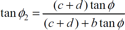
Now using the fact that wheel axes must intersect at a point when the mobile robot turns. Thus we get

$$\tan {\varphi }_1=\frac{(c+d)\tan \varphi }{(c+d)-b\tan \varphi }$$

and

$$\tan {\varphi }_2=\frac{(c+d)\tan \varphi }{(c+d)+b\tan \varphi }$$

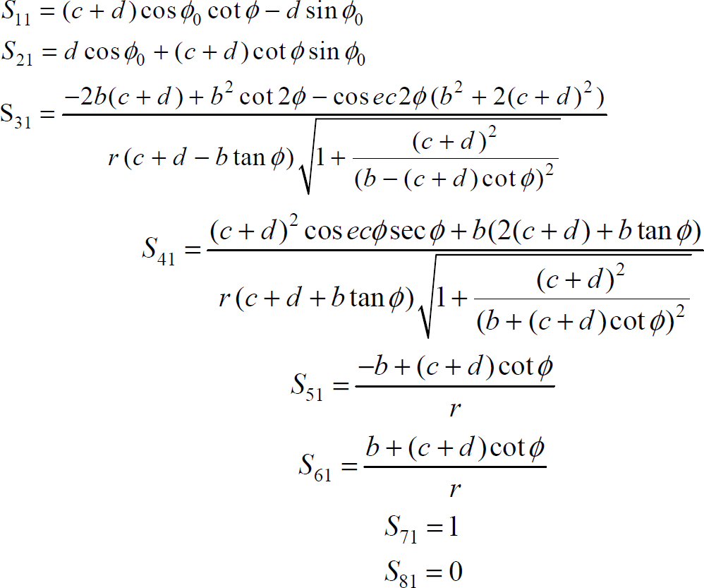
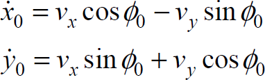
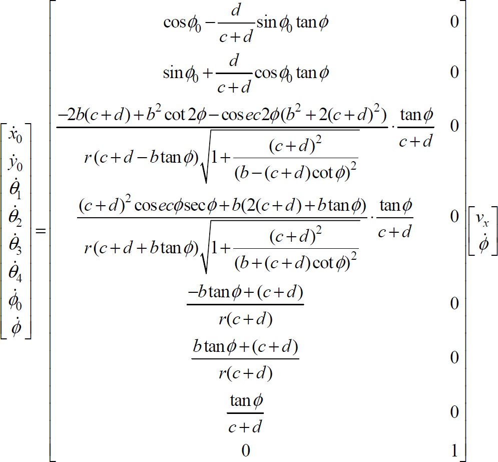
We introduce a vector of quasi velocities instead of generalized velocities because control runs in an abstract space. Quasi-velocities are function of kinematic parameters. Since the generalised velocities is always in the null space of A(q) according to (1) the generalized velocities q can be expressed in terms of quasi-velocities v(t) as follows

$$\dot{q}=s(q)v(t)$$

(2)

where s(q) is a 8 × 2 full rank matrix, whose columns are in the null space of A(q) and is given by (using the MATHEMATICA package)

$$s(q)=\left[\begin{array}{cc}{S}_{11}& 0\\ S_{21}& 0\\ S_{31}& 0\\ S_{41}& 0\\ S_{51}& 0\\ S_{61}& 0\\ S_{71}& 0\\ S_{81}& 1\end{array}\right]$$

Where

$$\begin{array}{l}{S}_{11}=(c+d)\cos {\varphi }_0\cot \varphi -d\sin {\varphi }_0\\ S_{21}=d\cos {\varphi }_0+(c+d)\cot \varphi \sin {\varphi }_0\\ S_{31}=\frac{-2b(c+d)+b^2\cot 2\varphi -\cos ec2\varphi (b^2+2{(c+d)}^2)}{r(c+d-b\tan \varphi )\sqrt{1+\frac{{(c+d)}^2}{{(b-(c+d)\cot \varphi )}^2}}}\\ S_{41}=\frac{{(c+d)}^2\cos ec\varphi \sec \varphi +b(2(c+d)+b\tan \varphi )}{r(c+d+b\tan \varphi )\sqrt{1+\frac{{(c+d)}^2}{{(b+(c+d)\cot \varphi )}^2}}}\\ S_{51}=\frac{-b+(c+d)\cot \varphi }{r}\\ S_{61}=\frac{b+(c+d)\cot \varphi }{r}\\ S_{71}=1\\ S_{81}=0\end{array}$$

Define

$$\begin{array}{l}{\dot{x}}_0=v_x\cos {\varphi }_0-v_y\sin {\varphi }_0\\ {\dot{y}}_0=v_x\sin {\varphi }_0+v_y\cos {\varphi }_0\end{array}$$

where v _x and v _y are the velocities of the centre of gravity of the mobile platform along the x and y-axes respectively. Thus we get

$$\left[\begin{array}{c}{\dot{x}}_0\\ {\dot{y}}_0\\ {\dot{\theta }}_1\\ {\dot{\theta }}_2\\ {\dot{\theta }}_3\\ {\dot{\theta }}_4\\ {\dot{\varphi }}_0\\ \dot{\varphi }\end{array}\right]=\left[\begin{array}{cc}\cos {\varphi }_0-\frac{d}{c+d}\sin {\varphi }_0\tan \varphi & 0\\ \sin {\varphi }_0+\frac{d}{c+d}\cos {\varphi }_0\tan \varphi & 0\\ \frac{-2b(c+d)+b^2\cot 2\varphi -\cos ec2\varphi (b^2+2{(c+d)}^2)}{r(c+d-b\tan \varphi )\sqrt{1+\frac{{(c+d)}^2}{{(b-(c+d)\cot \varphi )}^2}}}\cdot \frac{\tan \varphi }{c+d}& 0\\ \frac{{(c+d)}^2\cos ec\varphi \sec \varphi +b(2(c+d)+b\tan \varphi )}{r(c+d+b\tan \varphi )\sqrt{1+\frac{{(c+d)}^2}{{(b+(c+d)\cot \varphi )}^2}}}\cdot \frac{\tan \varphi }{c+d}& 0\\ \frac{-b\tan \varphi +(c+d)}{r(c+d)}& 0\\ \frac{b\tan \varphi +(c+d)}{r(c+d)}& 0\\ \frac{\tan \varphi }{c+d}& 0\\ 0& 1\end{array}\right]\left[\begin{array}{c}{v}_x\\ \dot{\varphi }\end{array}\right]$$

Since the control objective for the robot is to ensure that q(t) tracks a reference position and orientation denoted by q _d (t) = [x _d (t), y _d (t), φ_d0(t)] so we consider only

$$\left[\begin{array}{c}{\dot{x}}_0\\ {\dot{y}}_0\\ {\dot{\varphi }}_0\\ \dot{\varphi }\end{array}\right]=\left[\begin{array}{cc}\cos {\varphi }_0-\frac{d}{c+d}\sin {\varphi }_0\tan \varphi & 0\\ \sin {\varphi }_0-\frac{d}{c+d}\cos {\varphi }_0\tan \varphi & 0\\ \frac{\tan \varphi }{c+d}& 0\\ 0& 1\end{array}\right]\left[\begin{array}{c}{v}_1\\ v_2\end{array}\right]$$

(3)

Where v₁ = v _x and $v_2=\dot{\varphi }$

2.6 Chained form

In order to convert the kinematic model of the mobile robot in chained form following change of co-ordinates is used.

$$\begin{array}{l}{x}_1=x_0-d\cos {\varphi }_0\\ x_2=\frac{\tan \varphi }{(c+d){\cos }^3{\varphi }_0}\\ x_3=\tan {\varphi }_0\\ x_4=y_0-d\sin {\varphi }_0\end{array}$$

Together with two input transformations

$$\begin{array}{l}{V}_1=\frac{u_1}{\cos {\varphi }_0}\\ V_2=\frac{-3{\sin }^2\varphi \sin {\varphi }_0}{(c+d){\cos }^2{\varphi }_0}{u}_1+(c+d){\cos }^3{\varphi }_0{\cos }^2\varphi u_2\end{array}$$

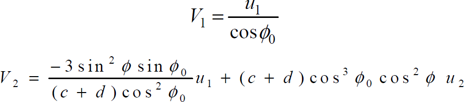
Then from above transformation we get the following two input four state chained form

$$\begin{array}{l}{\dot{x}}_1=u_1\\ {\dot{x}}_2=u_2\\ {\dot{x}}_3=x_2{u}_1\\ {\dot{x}}_4=x_3{u}_1\end{array}$$

(4)

where x = (x₁, x₂, x₃, x₄) is the state and u₁ and u₂ are the two control inputs.

3. Design of trajectory tracking controller

Denote the tracking error as x _e = x - x _d . The error differential equation are

$$\begin{array}{l}{\dot{x}}_{e1}=u_1-u_{d1}\\ {\dot{x}}_{e2}=u_2-u_{d2}\\ {\dot{x}}_{e3}=x_{e2}{u}_{d1}+x_2(u_1-u_{d1})\\ {\dot{x}}_{e4}=x_{e3}{u}_{d1}+x_3(u_1-u_{d1})\end{array}$$

(5)

The goal is to find a, Lipschitz continuous time-varying state-feedback controller $\tilde{u}$ i.e

$$u=\left[\begin{array}{c}{u}_1\\ u_2\end{array}\right]=\tilde{u}(x_e,u_{d1},u_{d2})$$

such that the tracking error x _e converges to zero asymptotically, i.e $\stackrel{t\to \infty }{lim}|x-x_d|=0$ under appropriate conditions on the reference control functions u_d1 and u_d2 and initial tracking errors x _e (0), with a good choice of Λ.

We first introduce a change of coordinates and rearrange system (5) into a triangular –like form so that the integrator backstepping can be applied.

Denote ${\tilde{x}}_d=(x_{d2},x_{d3})$ and let ${\eta }_1(.;{\tilde{x}}_d):R^4\to R^4$ be the mapping defined by

$$\begin{array}{l}{\zeta }_i=x_{e(4-i+1)}-(x_{e(n-i)}+x_{d(n-i)})x_{e1},1\le i\le 2\\ {\zeta }_3=x_{e2}\\ {\zeta }_4=x_{e1}\end{array}$$

In the new coordinates ζ = (ζ₁, ζ₂, ζ₃, ζ₄) system (5) is transformed into

$$\begin{array}{l}{\dot{\zeta }}_1=u_{d1}{\zeta }_2-x_2(u_1-u_{d1}){\zeta }_4\\ {\dot{\zeta }}_2=u_{d1}{\zeta }_3-u_2{\zeta }_4\\ {\dot{\zeta }}_3=u_2-u_{d2}\\ {\dot{\zeta }}_4=u_1-u_{d1}\end{array}$$

(6)

The basic design idea for backstepping based control law is to take for every lower dimension subsystem, some state variables as virtual control inputs and at the same time, recursively select an appropriate Lyapunov function candidate. Thus each step results in a new virtual control -er. In the end of the overall procedure, the true control law results which achieves the original design objective.

Consider the ζ₁ - subsystem of (6)

$${\dot{\zeta }}_1=u_{d1}{\zeta }_2-x_2(u_1-u_{d1}){\zeta }_4$$

(7)

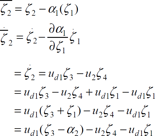
We consider the variable ζ₂ as virtual control input and the variable u_d1 and ζ₄ as time varying functions.

Denote ${\bar{\zeta }}_1={\zeta }_1$

Differentiating the function $V_1=\frac{1}{2}{\overline{{\zeta }_1}}^2$ along the solution of (6) yields

$${\dot{V}}_1=u_{d1}\overline{{\zeta }_1}{\zeta }_2-x_2\overline{{\zeta }_1}(u_1-u_{d1}){\zeta }_4$$

(8)

Since the variable ζ₂ is a virtual control input.

Selecting ζ₂ = -k₁ζ₁ k₁ ≥ 0

${\dot{V}}_1=-k_1{u}_{d1}^2{\overline{{\zeta }_1}}^2$ whenever ζ₄ = 0.

From above equation we observe that function α₁(ζ₁) = 0 is a stabilizing function i.e the desired value of virtual control ζ₂ for which V₁ is negative semi definite for subsystem (7). This desired value is called stabilizing function and ζ₂ is called virtual control. As in this case

$${\dot{V}}_1=-2k_1{u}_{d1}^2{V}_1$$

Above implies that

$$\begin{array}{l}{V}_1\to 0ast\to \infty \\ {\xi }_1\to 0ast\to \infty \\ i.e{V}_{1\lim }=0\end{array}$$

So the origin ζ₂ = 0 is asymptotically stable. Hence the function α₁(ζ₁) = 0 is a stabilizing function.

Define $\overline{{\zeta }_2}={\zeta }_2-{\alpha }_1({\zeta }_1)$

Differentiating the function

$$V_2=V_1+\frac{1}{2}{\overline{{\zeta }_2}}^2=\frac{1}{2}{\overline{{\zeta }_1}}^2+\frac{1}{2}{\overline{{\zeta }_2}}^2$$

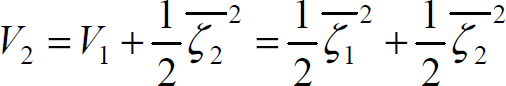
along the solution of (6) yields

$${\dot{V}}_2=u_{d1}\overline{{\zeta }_2{\zeta }_3}-x_2\overline{{\zeta }_1}(u_1-u_{d1}){\zeta }_4-u_2\overline{{\zeta }_2}{\zeta }_4$$

As

$$\begin{array}{l}\overline{{\zeta }_2}={\zeta }_2-{\alpha }_1({\zeta }_1)\\ {\dot{\stackrel{̄}{\zeta }}}_2={\dot{\zeta }}_2-\frac{\partial {\alpha }_1}{\partial {\zeta }_1}{\dot{\zeta }}_1\\ ={\dot{\zeta }}_2=u_{d1}{\zeta }_3-u_2{\zeta }_4\\ =u_{d1}{\zeta }_3-u_2{\zeta }_4+u_{d1}{\zeta }_1-u_{d1}{\zeta }_1\\ =u_{d1}({\zeta }_3+{\zeta }_1)-u_2{\zeta }_4-u_{d1}{\zeta }_1\\ =u_{d1}({\zeta }_3-{\alpha }_2)-u_2{\zeta }_4-u_{d1}{\zeta }_1\end{array}$$

Where

$${\alpha }_2({\zeta }_1,{\zeta }_2)=-{\zeta }_1$$

Again define

$$\begin{array}{l}\overline{{\zeta }_3}={\zeta }_3-{\alpha }_2({\zeta }_1,{\zeta }_2)\\ {\dot{\stackrel{̄}{\zeta }}}_3={\dot{\zeta }}_3-(\frac{\partial {\alpha }_2}{\partial {\zeta }_1}{\dot{\zeta }}_1+\frac{\partial {\alpha }_2}{\partial {\zeta }_2}{\dot{\zeta }}_2)\\ ={\dot{\zeta }}_3-(-{\dot{\zeta }}_1)={\dot{\zeta }}_3+{\dot{\zeta }}_1\\ =u_2-u_{d2}+u_{d1}{\zeta }_2-x_2(u_1-u_{d1}){\zeta }_4\end{array}$$

Consider the positive definite and proper function

$$V_3=V_2+\frac{1}{2}{\overline{{\zeta }_3}}^2=\frac{1}{2}{\overline{{\zeta }_1}}^2+\frac{1}{2}{\overline{{\zeta }_2}}^2+\frac{1}{2}{\overline{{\zeta }_3}}^2$$

Differentiating the function V₃ along the solution of (6) yields

$$\begin{array}{l}{\dot{V}}_3=\overline{{\zeta }_3}(u_{d1}\overline{{\zeta }_2}+u_2-u_{d2}+u_{d1}{\zeta }_2)\\ -(x_2\overline{{\zeta }_1}+x_2\overline{{\zeta }_3})(u_1-u_{d1}){\zeta }_4-u_2\overline{{\zeta }_2}{\zeta }_4\end{array}$$

In order to make V₃ negative definite we choose the following control input

$$u_{d1}\overline{{\zeta }_2}+u_2-u_{d2}+u_{d1}{\zeta }_2=-c_3\overline{{\zeta }_3}$$

(9)

where c₃ > 0.

Thus we have

$${\dot{V}}_3=-c_3{\overline{{\zeta }_3}}^2-(x_2\overline{{\zeta }_1}+x_2\overline{{\zeta }_3})(u_1-u_{d1}){\zeta }_4-u_2\overline{{\zeta }_2}{\zeta }_4$$

Finally consider the positive definite and proper function which serves as a candidate Lyapunov function for the whole system (6)

$$V_4=V_3+\frac{\lambda }{2}{\zeta }_4^2=\frac{1}{2}{\overline{{\zeta }_1}}^2+\frac{1}{2}{\overline{{\zeta }_2}}^2+\frac{1}{2}{\overline{{\zeta }_3}}^2+\frac{\lambda }{2}{\zeta }_4^2$$

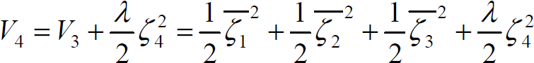
Where Λ > 0 is a design parameter.

Differentiating the function V₄ along the solution of (6) yields

$$\begin{array}{l}{\dot{V}}_4=-c_3{\overline{{\zeta }_3}}^2-(x_2\overline{{\zeta }_1}+x_2\overline{{\zeta }_3})(u_1-u_{d1}){\zeta }_4-u_2\overline{{\zeta }_2}{\zeta }_4+\\ \lambda {\zeta }_4(u_1-u_{d1})\\ {\dot{V}}_4=-c_3{\overline{{\zeta }_3}}^2+[\{\lambda -(x_2\overline{{\zeta }_1}+x_2\overline{{\zeta }_3})\}(u_1-u_{d1})-u_2\overline{{\zeta }_2}]{\zeta }_4\end{array}$$

In order to make V₄ negative definite we choose the following control input

$$\{\lambda -(x_2\overline{{\zeta }_1}+x_2\overline{{\zeta }_3})\}(u_1-u_{d1})-u_2\overline{{\zeta }_2}=-c_4{\zeta }_4$$

(10)

From (9) and (10) we get the following control law

$$\begin{array}{l}{u}_1=u_{d1}+\frac{-c_4{\zeta }_4+u_2{\zeta }_2}{\lambda -(2x_2{\zeta }_1+x_2{\zeta }_3)}\\ u_2=u_{d2}-c_3({\zeta }_3+{\zeta }_1)-2u_{d1}{\zeta }_2\end{array}$$

4. Simulation results

To examine the effectiveness of the proposed trajectory tracking control methodology, the simulation for a four wheeled mobile robot were performed in MATHEMATICA. The system parameters of the four wheel mobile robot were selected as c=1.3m, d=1.4 m, 2b=1.5m.

4.1. Tracking a straight line

Tracking a straight line is a simple case for all robots. Here for simulation we consider that the straight line. We choose the following as design parameters Λ = 5, c₃ = c₄ = 2 for tracking a straight line. It is further assumed that initially x _e (0) = (2, 0.8, 0.8, 0.8).

The straight line reference trajectory to be tracked is given by x _d (t) = t, y _d (t) = 0.

The desired trajectory and the norm of the tracking error is shown in Fig. 3 and fig.4 respectively.

Fig.3:

Desired straight line trajectory

Fig.4:

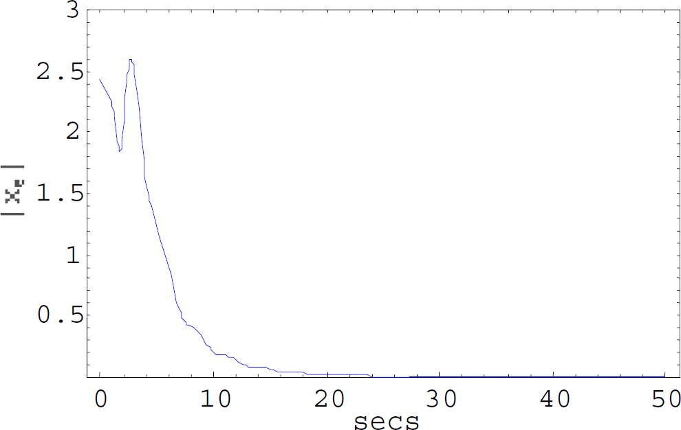
Norm of tracking error x _e (t) versus time

4.2. Tracking the curve xd(t) = t, yd(t) = a sin ωt

we consider the following desired sinusoidal trajectory x _d (t) = t, y _d (t) = a sin ωt as shown in Fig. 5.

Fig.5:

Desired sinusoidal trajectory

Fig.7 demonstrates the evolution of the norm of the tracking error x _e (t) based on the following choice of design parameters and initial condition:

$$\lambda =3,c_3=c_4=5,x_e(0)=(2,0.5,0.5,1.5)$$

with a=0.2 and ω=0.5.

Fig.6

Desired steering angle versus time

Fig.7:

Norm of tracking error x _e (t) versus time

5. Conclusion

In this paper the nonholonomic constraints and the kinematics model of the four wheel (front steering and rear driving) mobile robot under pure rolling and no side slipping condition is derived. Using the change of coordinates the system is transformed into chained form and then a backstepping based tracking controller is derived. Simulation results are presented with two examples to illustrate the approach.