Sage Journals: Discover world-class research

Abstract

This research is aimed to the development of a dynamic control to enhance the performance of the existing dynamic controllers for mobile robots. System dynamics of the car-like robot with nonholonomic constraints were employed. A Backstepping approach for the design of discontinuous state feedback controller is used for the design of the controller. It is shown that the origin of the closed loop system can be made stable in the sense of Lyapunov. The control design is made on the basis of a suitable Lyapunov function candidate. The effectiveness of the proposed approach is tested through simulation on a car-like vehicle mobile robot.

Keywords

backstepping approach mobile robot chained form systems nonholonomic systems

1. Introduction

Wheeled mobile robots (WMRs) are increasingly present in industrial and service robotics, particularly when flexible motion capabilities are required on reasonably smooth ground and surfaces (Scraft & Schmier, 1998). Several mobility configurations can be found in these applications. The most common are the tricycle and the car-like drive. Kinematics study of several configurations of WMRs can be found in (Alexander & Maddocks, 1989).

Beside the relevance in industrial applications, the problem of autonomous motion planning and control of WMRs has attracted the interest of researchers in view of its theoretical challenges. In particular, these systems are typically examples of nonholonomic mechanical systems (Neimark & Fufaev, 1992).

In the absence of workspace obstacles, the basic motion tasks assigned to a WMR may be reduced to moving between two postures and following a given trajectory. From a control viewpoint, the peculiar nature of nonholonomic kinematics makes the control problem easier than the first; in fact, it is known (Campion et al. 1991), that feedback stabilization at a given posture cannot be achieved via smooth time invariant control. This indicates that the problem is really nonlinear; linear control is ineffective, even locally, and innovative design is required.

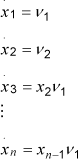
The trajectory tracking problem of WMRs was globally solved in (Samson & Ait Abderrahim, 1991) by using nonlinear feedback control, and independently in (De Luca & Benedetto, 1993) and (D'arendra & Bastin, 1995) through the use of dynamic feedback linearization. Recursive backstepping control schemes for chained forms of WMRs have been also addressed by several authors (Jiang & Nijimar, 1999), (Tayebi et al. 1997). It can be shown that the dynamic equations of a car-like vehicle mobile robot can be written in chained form as:

\begin{array}{l} {\dot{x}}_{1} = v_{1} \\ {\dot{x}}_{2} = v_{2} \\ {\dot{x}}_{3} = x_{2} v_{1} \\ ⋮ \\ {\dot{x}}_{n} = x_{n - 1} v_{1} \end{array}

(1)

where x = (x₁, x₂,…,x_n) ^T ∈ ℛ ⁿ denotes the state vector and v = (v₁, v₂) ^T ∈ ℛ² is the control input vector. Such a class of nonlinear systems can not be stabilized via continuous based time-invariant systems (Brockett, 1993) which motivated the search of other stabilizing controls for this type of systems. Kolmanovsky and Mc-Clamroch (Klamanovsky & Mc Clamroch, 1995) stated the art of existing solution for nonholonomic systems. In the recent last few years many authors exhibit a particular attention to the design of discontinuous controller for chained systems, (Tayebi et al, 1997), (Tanner & Kyriakopoulos, 2002)

In this paper we propose a systematic backstepping based procedure for the design of a discontinuous time-invariant controller for nonholonomic chained forms with application to nonholonomic mobile robot systems. It is shown that backstepping control for chained form systems can guarantee the boundedness of the whole state and makes the origin of the closed-loop system exponentially attractive provided that the initial states belong to the set defined by:

Ω_{0} : Ω_{0} = {{(x_{1} (0), x_{2} (0), \dots, x_{n} (0))}^{T} \in ℜ^{n} / x_{1} (0) \neq 0}

(2)

The proposed control scheme is applied to the dynamics of a car-like vehicle mobile robot which investigation and reduction are presented exhaustively in section 2.

2. Dynamic Model and Reduction of Nonholonomic Mechanical Systems

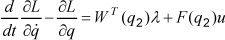
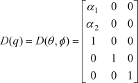
Consider a Lagrangian system with n-dimensional configuration vector q, a force matrix F (q) and m (m < n) nonholonomic first order constraints defined by:

W^{T} (q) \dot{q} = 0,

(3)

that are non-integrable, i.e. there is no h(t): ḣ = W^T (q)q̇ and where W ∈ ℛ^n×n is the constraint equation, then the dynamics of the nonholonomic system can be written as

\frac{d}{d t} \frac{\partial L (q, \dot{q})}{\partial \dot{q}} - \frac{\partial L (q, \dot{q})}{\partial q} = W^{T} (q) λ + F (q) u

(4)

W (q) \dot{q} = 0

(5)

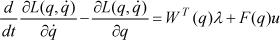
Where L(q, q̇) is the system Lagrangian, u ∈ ℛ^l is the control input, such that l = rank(F(q)), and Λ ∈ ℛ ^m is the vector of Lagrange multipliers. Since m ≥ 1 then we have necessarily l ≤ n – 1. The term W^T Λ represents the effect of the constrained forces. This is based on the principle of virtual forces which states that the constraint forces do not work on motions allowed by constraints.

The system (4)–(5) is called a mechanical system with first order nonholonomic constraints. Nonholonomic systems in the form (4)–(5) with F(q) = 0 are called Caplygin systems.

Assumption 1

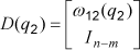
Assume W (q) has full row rank. Then q can be partitioned as (q₁, q₂)^T such that W (q) = (W₁(q), W₂(q))^T where W₁(q) is an invertible matrix. Therefore the constraint equation (3) can be rewritten as

W_{1} (q) {\dot{q}}_{1} + W_{2} (q) {\dot{q}}_{2} = 0

(6)

Assumption 2

We assume that the system generalized mass matrix M(q), F(q) and W(q) are all independent of q₁.

Note that M (q) can be directly obtained from the relation $L (q, \dot{q}) = \frac{1}{2} {\dot{q}}^{T} M (q) \dot{q} - V (q)$ , where V(q) is the potential energy of the system.

Assumption 3

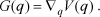
Assume the potential energy of the system V(q) is in the form

V (q) = K_{v}^{T} q_{1} + U (q_{2})

(7)

where k_v ∈ ℛ ^n–m is a constant vector and U is a scalar function.

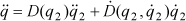
Under the above assumptions, the dynamics of the underactuated nonholonomic system (4)–(5) can be expressed as

\frac{d}{d t} \frac{\partial L}{\partial \dot{q}} - \frac{\partial L}{\partial q} = W^{T} (q_{2}) λ + F (q_{2}) u

(8)

W_{1} (q) {\dot{q}}_{1} + W_{2} (q) {\dot{q}}_{2} = 0

(9)

To eliminate Λ from (8), one can multiply both sides of the forced Euler-Lagrange equation in (5) by a matrix A(q) that annihilates W^T(q), i.e. A(q)W^T(q) = 0. For doing so, let us define

ω_{12} (q_{2}) = - W_{1}^{- 1} (q_{2}) W_{2} (q_{2})

(10)

then

\dot{q} = D (q_{2}) {\dot{q}}_{2}

(11)

where

D (q_{2}) = [\begin{array}{l} ω_{12} (q_{2}) \\ I_{n - m} \end{array}]

(12)

where I_n–m is the n–m identity matrix. By direct calculation, it can be readily shown that A(q₂) = D^T(q₂) annihilates W^T(q₂). This eventually leads to the following reduction theorem for underactuated nonholonomic systems with symmetry.

Theorem 1

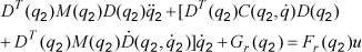
Consider the underactuated mechanical control system with nonholonomic constraints and symmetry in (8)–(9). Then (8)–(9) with (2n + m) first-order equations can be reduced to a system of (2n - m) first-order equations in the following cascade form.

{\dot{q}}_{x} = ω_{r} (q_{r}) {\dot{q}}_{r}

(13)

M_{r} (q_{r}) {\overset{..}{q}}_{r} + C_{r} (q_{r}, {\dot{q}}_{r}) {\dot{q}}_{r} + G_{r} (q_{r}) = F_{r} (q_{r}) u

(14)

where

(q_{x}, q_{r}) = (q_{1}, q_{2}), ω_{r} (q_{r}) = ω_{12} (q_{2}),

and

\begin{array}{l} M_{r} (q_{r}) = D {(q_{2})}^{T} M (q_{2}) D (q_{2}) \\ G_{r} (q_{r}) = ω_{r}^{T} (q_{r}) k_{v} + \nabla_{q r} U (q_{r}) \\ C_{r} (q_{r}, {\dot{q}}_{r}) : = D^{T} (q_{2}) C (q_{2}, \dot{q}) D (q_{2}) + D^{T} (q_{2}) M (q_{2}) \dot{D} (q_{2}, {\dot{q}}_{2}) \\ F_{r} (q_{r}) = D^{T} (q_{2}) F (q_{2}) \end{array}

(15)

Moreover, if V(q) = U(q₂) i.e. k_v = 0 in (7), the reduced system is a well defined Lagrangian system with configuration vector q_r = q₂ and the Lagrangian function

L_{r} (q_{r}, {\dot{q}}_{r}) = \frac{1}{2} {\dot{q}}_{r}^{T} M_{r} (q_{r}) {\dot{q}}_{r} - U (q_{r})

(16)

which satisfies a forced Euler-Lagrange equation in cascade with the constraint equation as the following

\begin{array}{l} {\dot{q}}_{x} = ω_{r} (q_{r}) {\dot{q}}_{r} \\ \frac{d}{d t} \frac{\partial L_{r}}{\partial {\dot{q}}_{r}} - \frac{\partial L_{r}}{\partial q_{r}} = F_{r} (q_{r}) u \end{array}

(17)

In addition, if l + m < n or l + m = n, then the reduced system with configuration vector q_r is an underactuated (or fully actuated) mechanical system.

Proof. The forced Euler-Lagrange equation in (8) can be rewritten as

M (q_{2}) \overset{..}{q} + C (q_{2}, \dot{q}) \dot{q} + G (q) = W^{T} (q_{2}) λ + F (q_{2}) u

(18)

Where C(q2, q̇) satisfies

\dot{M} = C + C^{T}

and G(q) such that

G (q) = \nabla_{q} V (q) .

Multiplying both sides of the last equation by A(q₂) = D^T (q₂) eliminates Λ and gives

D^{T} (q_{2}) M (q_{2}) \overset{..}{q} + D^{T} (q_{2}) C (q_{2}, \dot{q}) \dot{q} + G_{r} (q) = F_{r} (q_{2}) u

(19)

where F_r(q₂) = D^T (q₂)F(q₂) and

\begin{array}{l} G_{r} (q_{2}) = D^{T} (q_{2}) G (q) & = [ω_{12}^{T} (q_{2}) I] [\begin{array}{l} \nabla_{q_{1}} V (q) \\ \nabla_{q_{2}} V (q) \end{array}] \\ = ω_{12}^{T} (q_{2}) k + \nabla_{12} U (q 2) = : G_{r} (q_{2}) \end{array}

on the other hand, taking the derivative of q̇ = D(q₂)q̇₂ implies

\overset{..}{q} = D (q_{2}) {\overset{..}{q}}_{2} + \dot{D} (q_{2}, {\dot{q}}_{2}) {\dot{q}}_{2}

Substituting q̈ in (19), we get

\begin{array}{l} D^{T} (q_{2}) M (q_{2}) D (q_{2}) {\overset{..}{q}}_{2} + [D^{T} (q_{2}) C (q_{2}, \dot{q}) D (q_{2}) \\ + D^{T} (q 2) M (q_{2}) \dot{D} (q_{2}, {\dot{q}}_{2})] {\dot{q}}_{2} + G_{r} (q_{2}) = F_{r} (q_{2}) u \end{array}

by taking q_r = q₂, this last equation can be rewritten as

M_{r} (q_{r}) {\overset{..}{q}}_{r} + C_{r} (q_{r}, {\dot{q}}_{r}) {\dot{q}}_{r} + G_{r} (q_{r}) = F_{r} (q_{r}) u

(20)

where

M_{r} (q_{r}) : = D^{T} (q_{2}) M (q_{2}) D (q_{2})

(21)

\begin{array}{l} C_{r} (q_{r}, {\dot{q}}_{r}) : = D^{T} (q_{2}) C (q_{2}, \dot{q}) D (q_{2}) \\ + D^{T} (q_{2}) M (q_{2}) \dot{D} (q_{2}, {\dot{q}}_{2}) \end{array}

(22)

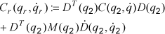
To establish that (20) is in fact equivalent to the forced Euler-Lagrange equation for the reduced system with the Lagrangian function L_r(q_r, q̇_r) and the force matrix F_r(q_r), we need to prove that C_r(q_r, q̇_r) satisfies Ṁ_r = C_r + C^T_r. By direct calculation we have

\begin{array}{l} {\dot{M}}_{r} & = D^{T} \dot{M} D + {\dot{D}}^{T} M D + D^{T} M \dot{D} \\ = D^{T} (C + C^{T}) D + {\dot{D}}^{T} M \dot{D} + D^{T} M \dot{D} \\ = (D^{T} C D + D^{T} M \dot{D}) + (D^{T} C^{T} D + {\dot{D}}^{T} M D) \\ = C_{r} + C_{r}^{T} \end{array}

and the result follows.

3. The Car-like Vehicle

In this section, we address reduction of the dynamic model of a car-like vehicle as shown in Figure 1. The dynamic model of a car is an example of underactuated nonholonomic systems with five degrees of freedom, two control inputs and two velocity constraints. Let q = (x, y, θ, Ψ, ϕ) denote the configuration vector of the system. (x, y) denote the position of the center of the axle between the two rear wheels, θ is the orientation of the car body with respect to x-axis, ψ is the angle of rotation of each wheel and ϕ is the steering angle with respect the car body. The distance between the rear and front wheels axles is denoted by l and r denotes the radius of the wheels

Fig.1.

A car-like vehicle

The velocity constraints of the front and rear wheels are given by

\begin{array}{l} sin (θ + ϕ) \frac{d}{d t} (x + l cos θ) - cos (θ + ϕ) \frac{d}{d t} (x + l sin θ) = 0 \\ sin (θ) \dot{x} - cos (θ) \dot{y} = 0 \end{array}

(23)

\begin{array}{l} sin (θ + ϕ) \dot{x} - cos (θ + ϕ) \dot{y} - l cos ϕ \dot{θ} = 0 \\ sin (θ) \dot{x} - cos (θ) \dot{y} = 0 \end{array}

(24)

These two constraints can be rewritten as W(q)q̇ = 0 where W = (W₁, W₂) is partitioned according to q_x = (x, y) and q_r = (θ, ψ, ϕ). The matrices W₁ and W₂ are given by

W_{1} (θ, ϕ) = [\begin{array}{l} sin (θ + ϕ) - cos (θ + ϕ) \\ sin (θ) cos (θ) \end{array}]

and

W_{2} (θ, ϕ) = [\begin{array}{l} - l cos ϕ 0 0 \\ 0 0 0 \end{array}]

(25)

Note that W₁ is not invertible at ϕ = 0.

Define now

ω_{12} (θ, ϕ) = - W_{1}^{- 1} W_{2} = [\begin{array}{l} α_{1} 0 0 \\ α_{2} 0 0 \end{array}]

where

α_{1} (θ, ϕ) = \frac{l cos θ}{tan ϕ}, α_{2} (θ, ϕ) = \frac{l sin θ}{tan ϕ}

And D(q) can then be determined from ω₁₂(θ,ϕ) as

D (q) = D (θ, ϕ) = [\begin{array}{l} α_{1} & 0 & 0 \\ α_{2} & 0 & 0 \\ 1 & 0 & 0 \\ 0 & 1 & 0 \\ 0 & 0 & 1 \end{array}]

(26)

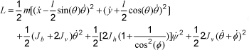
The Lagrangian of the dynamic car is given by

\begin{array}{l} L = & \frac{1}{2} m [{(\dot{x} - \frac{l}{2} sin (θ) \dot{θ})}^{2} + {(\dot{y} + \frac{l}{2} cos (θ) \dot{θ})}^{2}] \\ + \frac{1}{2} (J_{b} + 2 J_{v}) {\dot{θ}}^{2} + \frac{1}{2} [2 J_{h} (1 + \frac{1}{{cos}^{2} (ϕ)})] ψ^{2} + \frac{1}{2} 2 J_{v} {(\dot{θ} + \dot{ϕ})}^{2} \end{array}

(27)

where m is the mass of the car, J_b is the inertia of the body, J_h is the inertia of each wheel along the horizontal axes and J_v is the inertia of each wheel in the vertical axes. The Lagrangian can be expressed as

L = \frac{1}{2} {\dot{q}}^{T} [\begin{matrix} m & 0 & - m l / 4 sin θ & 0 & 0 \\ 0 & m l / 4 cos θ & m_{c} & 0 & 0 \\ - m l / 4 sin θ & m l / 4 sin θ & J_{θ} & 0 & 2 J_{v} \\ 0 & 0 & 0 & J_{h}^{'} & 0 \\ 0 & 0 & 2 J_{v} & 0 & 2 J_{v} \end{matrix}] \dot{q}

where

J_{θ} = J_{b} + 4 J_{v} + \frac{m l^{2}}{4}, J_{h}^{'} = 2 J_{h} (2 + {tan}^{2} (ϕ))

The differential-algebraic equations of motion of the dynamic car are such as

\frac{d}{d t} \frac{\partial L}{\partial \dot{q}} - \frac{\partial L}{\partial q} = W^{T} (q) [\begin{matrix} λ_{1} \\ λ_{2} \end{matrix}] + [\begin{matrix} 0_{3 \times 2} \\ I_{2 \times 2} \end{matrix}] [\begin{matrix} u_{1} \\ u_{2} \end{matrix}]

(29)

where (Λ₁, Λ₂) ∈ ℛ × ℛ are the Lagrange multipliers and (u₁, u₂) ∈ ℛ × ℛ are the torques applied to the rear wheels and the steering wheel respectively. The dynamics of the car in (29) can be reduced to the cascade of the constraint equation and a reduced Lagrangian system with configuration vector q = (θ, ψ, ϕ) as

M_{r} (q_{r}) {\overset{..}{q}}_{r} + C_{r} (q_{r}, {\dot{q}}_{r}) {\dot{q}}_{r} + G_{r} (q_{r}) = F_{r} (q_{r}) u

(30)

where

\begin{matrix} M_{r} = D^{T} M D \\ C_{r} = D^{T} C D + D^{T} M \dot{D} \\ F_{r} = D^{T} F \end{matrix}

By direct calculation and after simplification we get

F_{r} = [\begin{array}{l} 0 & 0 \\ 1 & 0 \\ 0 & 1 \end{array}]

and

M_{r} = M_{r} (ϕ) = [\begin{matrix} {\bar{J}}_{θ} (ϕ) & 0 & 2 J_{v} \\ 0 & 2 J_{h} (2 + {tan}^{2} (ϕ)) & 0 \\ 2 J_{v} & 0 & 2 J_{v} \end{matrix}]

(31)

with

{\bar{J}}_{θ} (ϕ) = J_{θ} + \frac{m l^{2}}{{tan}^{2} (ϕ)}

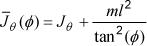
Clearly, the reduced Lagrangian is itself underactuated with three degrees of freedom (θ, ϕ, ψ) and two controls. In addition, (θ, ψ) are the external variables and ϕ is the shape variable of the car. The dynamics of the actuated variables (ϕ, ψ) of the reduced system can be linearized as

\begin{matrix} \overset{..}{ψ} = τ_{1} \\ \overset{..}{ϕ} = τ_{2} \end{matrix}

(32)

with τ₁ and τ₂ the new control inputs. Equation (32) can be obtained using an explicit collocated change of variable in the form

u = η (ϕ) τ + β (ϕ, {\dot{q}}_{r})

Where τ = [τ₁ τ₂]^T, β a scalar function, and

η (ϕ) = [\begin{matrix} 2 J_{h} (2 + {tan}^{2} (ϕ)) & 0 \\ 0 & 2 J_{v} (1 - \frac{2 J_{v} {tan}^{2} (ϕ)}{m l^{2} + J_{θ} {tan}^{2} (ϕ)} \end{matrix}]

(33)

η(ϕ) is well defined and positive definite for all ϕ.

From the first constraint equation, we can solve for θ to get

\dot{θ} = (\dot{x} cos θ + \dot{y} sin θ) tan ϕ

(34)

and the overall dynamics of the car can be written as

\begin{array}{l} \dot{x} = \dot{ψ} r cos θ \\ \dot{y} = \dot{ψ} r sin θ . \\ \dot{θ} = ψ \frac{r}{l} tan θ \\ \overset{..}{ψ} = τ_{1} \\ \overset{..}{ϕ} = τ_{2} \end{array}

(35)

where r is the radius of the wheel.

After normalization of the units of (x, y) by r, and taking

\dot{ψ} = ω_{1}

we get

\begin{array}{l} x = ω_{1} r cos θ \\ y = ω_{1} r sin θ \\ \dot{θ} = ω_{1} \frac{r}{1} tan θ \\ \dot{ϕ} = ω_{2} \end{array}

(36)

where

{\dot{ω}}_{1} = τ_{1}, {\dot{ω}}_{2} = τ_{2}

(37)

Applying the change of coordinates and control as:

\begin{array}{l} x_{1} = x \\ x_{2} = \frac{tan ϕ}{l {cos}^{3} θ} \\ x_{3} = tan θ \\ x_{4} = y \\ v_{1} = ω_{1} ϕ cos θ \\ v_{2} = \frac{1 + {tan}^{2} ϕ}{l {cos}^{3} θ} ω_{2} + \frac{3 tan θ {tan}^{2} ϕ}{l^{2} {cos}^{3} θ} \end{array}

(38)

transforms finally the nonholonomic system (38) into a chained form-type system of the form

\begin{array}{l} {\dot{x}}_{1} = v_{1} \\ {\dot{x}}_{2} = v_{2} \\ {\dot{x}}_{3} = x_{3} v_{1} \\ {\dot{x}}_{4} = x_{3} v_{1} \end{array}

(39)

where (x₁, …, x₄)^T ∈ ℛ⁴ are the states of the system and (v₁, v₂) ∈ ℛ² are the control inputs.

4. Backstepping control of the car-like vehicle

In order to apply the backstepping approach procedure, let us consider the following change of coordinates z_i = x_n–i+1, 1 ≤ i ≤ 4. System (39) becomes

\begin{array}{l} {\dot{z}}_{1} = z_{2} v_{1} \\ {\dot{z}}_{2} = z_{3} v_{1} \\ {\dot{z}}_{3} = v_{2} \\ {\dot{z}}_{4} = v_{1} \end{array}

(40)

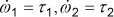
To guarantee the exponential convergence of z₄, we use a state feedback such that

v_{1} = - k_{4} z_{4},

where k₄ is a positive constant. System (40) becomes

\begin{array}{l} {\dot{z}}_{1} = - k_{4} z_{4} z_{2} \\ {\dot{z}}_{2} = - k_{4} z_{4} z_{3} \\ {\dot{z}}_{3} = v_{2} \\ \dot{z} = - k_{4} z_{4} \end{array}

(41)

Now the problem consists of finding a control law v₂ such that, if the initial state belongs to the set $Ω = {{(z_{1} (0), z_{2} (0), z_{3} (0), Z_{4} (0))}^{T} \in R^{4} / Z_{4} (0) = x_{1} (0) \neq 0}$ The whole state of the closed loop system remains bounded and converges exponentially to zero. The design procedure is to be done in 3 steps.

Step1

Consider the first equation of the system (41), where z₂ is viewed as a virtual control variable, and consider the Lyapunov function candidate

V_{1} = \frac{1}{2 k_{4}} z_{1}^{2}

(42)

the time derivative of (42) becomes

{\dot{V}}_{1} = - z_{1} z_{2} z_{4}

(43)

Using the following virtual control

η_{1} = k_{1} \frac{z_{1}}{z_{4}}

(44)

where k₁ is a positive constant, and substitute z₂ by η₁. Equation (43) becomes

{\dot{V}}_{1} = - k_{1} z_{1}^{2}

Step 2

We introduce a new variable ε₂ = z₂ – η₁, which represents the deviation between y₂ and the virtual control η₁ and consider the first two equations of (41) where z₂ is substituted by ε₂ + η₁ and z₃ is viewed as a virtual control variable, then

\begin{array}{l} \dot{z} = - k_{4} (ɛ_{2} + α_{1}) \\ {\dot{ɛ}}_{2} = - k_{4} z_{3} z_{4} - {\dot{α}}_{1} \end{array}

(45)

Using the Lyapunov function candidate

V_{2} = V_{1} + \frac{1}{2 k_{4}} ɛ_{2}^{2} = \frac{1}{2 k_{4}} z_{1}^{2} + \frac{1}{2 k_{4}} ɛ_{2}^{2}

(46)

The time derivative of (41) yields

{\dot{V}}_{2} = - z_{1} z_{4} (ɛ_{2} + η_{1}) - (z_{3} z_{4} + \frac{{\dot{η}}_{1}}{k_{4}}) ɛ_{2}

(47)

= {\dot{V}}_{1 - ɛ_{2}} (z_{3} z_{n} + \frac{η_{1}}{k_{4}}) - z_{1} z_{n} ɛ_{2}

(48)

By choosing the virtual control law η₂ which substitutes Z₃ as

η_{2} = - z_{1} + k_{2} \frac{ɛ_{2}}{z_{4}} - \frac{{\dot{η}}_{1}}{k_{4} z_{4}}

(49)

such that k₂ > 0, equation (48) becomes

{\dot{V}}_{2} = {\dot{V}}_{1} - k_{2} ɛ_{2}^{2} = - k_{1} z_{1}^{2} - k_{2} ɛ_{2}^{2}

(50)

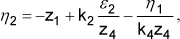
Step 3

Likewise in step 2 we introduce a new variable ε₃ such that:

ɛ_{3} = z_{3} - η_{2}

(51)

and using the Lyapunov function candidate

V_{3} = V_{2} + \frac{1}{2 k_{4}} ɛ_{3}^{2}

(52)

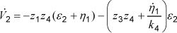
Evaluating the time derivative of (52), gives

{\dot{V}}_{3} = {\dot{V}}_{2} - k_{4} ɛ_{2} ɛ_{3} z_{4} + \frac{ɛ_{3}}{k_{4}} (v_{2} - {\dot{η}}_{2})

(53)

Under the following control law v₂ in (41), defined over Ω, as

v_{2} = - {\dot{η}}_{2} - k_{4} k_{3} ɛ_{3} + k_{4} z_{4} ɛ_{2}

(54)

where k₃ is a positive parameter and η₂ can be evaluated from the expression of η₂, equation (53) becomes

\begin{array}{l} {\dot{V}}_{3} = & {\dot{V}}_{2} - k_{3} ɛ_{3}^{2} \\ = - (k_{1} z_{1}^{2} + k_{2} ɛ_{1}^{2} + k_{3} ɛ_{2}^{2}) \end{array}

(55)

which is negative semi-definite function.

Now one can easily conclude that conclude that (z₁, ε₂, ε₃) ^T is bounded and tends to zero when t approaches the infinity. Therefore z_i → η_i–1, i = 2,3 when t → ∞. To guarantee the boundedness and the convergence to zero of (z₂, z₃) ^T , one must ensure the boundedness and convergence to zero of (η₁, η₂)^T. Since $η_{1} = k_{1} \frac{Z_{1}}{Z_{4}}$ , and that z₄ is assumed to be different from zero, then η₁ is bounded and converges to zero as t → ∞. On the other hand, $η_{2} = - Z_{1} + \frac{k_{2} ɛ_{2}}{z_{4}} - \frac{{\dot{η}}_{1}}{k_{4} Z_{4}},$ , this function is bounded and converges to zero if η₁ is also bounded and converges to zero. η₁ can be directly calculated as

{\dot{η}}_{1} = k_{1} \frac{{\dot{z}}_{1} z_{4} - {\dot{z}}_{4} z_{1}}{z_{4}^{2}}

(56)

which is also bounded and converges to zero when t → ⋡.

Finally we conclude that if z₄ (0) = x₁ (0) ≠ 0 then i)

The whole state remains in Ω since z₄ and then x₁ decays to zero

ii)

The state trajectory of the closed loop system is bounded and converges to zero

Now we can summarize the previous procedure in the following theorem

Theorem 1

Consider the system (39) with the control law

\begin{array}{l} v_{1} = {\begin{array}{l} - k_{4} x_{1} & for x_{1} (0) \neq 0 \\ v_{1}^{*} & for x_{1} (0) = 0 \end{array} \\ v_{2} = {\begin{array}{l} k_{4} ɛ_{2} x_{1} - k_{4} k_{3} ɛ_{3} + {\dot{η}}_{2} & for x_{1} (0) \neq 0 \\ v_{2}^{*} & for x_{1} (0) = 0 \end{array} \end{array}

where v₁^* ∈ ℛ / {0}, v₂^* ∈ ℛ /{0} are two constant values and where

η_{1} = k_{1} \frac{z_{1}}{z_{4}} and η_{2} = - z_{1} + k_{2} \frac{ɛ_{2}}{z_{4}} - \frac{{\dot{η}}_{1}}{k_{4} z_{4}}

with k_i > 0, i = 1, …, 4

then i)

the whole state z = (z₁, …, z₄)^T and equivalently x = (x₁, …, x₄)^T is bounded and decays to zero when t → ∞,

ii)

the control law is well defined for all t ≥ 0.

5. Simulation Results

The technique presented in this paper is tested on the system

\begin{array}{l} \dot{x} = v cos θ \\ \dot{y} = v sin θ \\ \dot{θ} = \frac{v}{l} tan θ \\ \dot{ϕ} = ω \end{array}

where v is the constant linear velocity of the car and l is the distance between the front and rear wheels axles.

Results are depicted in Figures 2–6. The Initial conditions are taken as

x (0) = {[x_{0}, y_{0}, θ_{0}, ϕ_{0}]}^{T} = {[1.5, 2, \frac{π}{4}, - \frac{π}{2}]}^{T}

and the following gains are used

k_{1} = 3, k_{2} = 2, k_{3} = 0.5 and k_{4} = 0.5.

Fig. 2.

Path to the origin of the mobile robot

Fig. 3

Time history of the variable x.

Fig. 4.

Time history of the variable y.

Fig. 5

Time history of the variable θ

Fig. 6

Time history of the variable ϕ.

Figure 2 shows the path traversed by the mobile robot. Figures 3–6 show the time behavior of the variable, x, y, θ and ϕ. It is clear that the discontinuous backstepping approach presented in this paper guarantees the convergence and the stabilization of all the states of the system.

6. Conclusions

This paper presents a novel technique for backstepping discontinuous control with application to the stabilization of a nonholonomic mobile robot. The methodology is not restricted, though to nonholonomic systems but can be applied to a broad class of strictly feedback discontinuous systems. The proposed control scheme is smooth everywhere except at x₁ = 0. The discontinuity involved in the control is not very restrictive since it occurs just for x₁(0) = 0. The simulation results made on a car-like mobile robot demonstrate the validity of the proposed control.

References

Alexander

J.C.

, and Maddocks

J.H.

, (1989), On the Kinematics of wheeled mobile robot, International Journal of Robotics Research. 8, 5, pp. 15–27.

d'Andrea-Novel

Bastin Campion

(1995), Control of nonholonomic wheeled mobile robots by state feedback linearization. International Journal of Robotics Research, 14, 6, pp. 543–559.

Brockett

R.W.

1993: Asymptotic stability and feedback stabilization. Progress in Math., vol. 27, Birkhauser, pp. 181–208, 1993.

Campion

d'Andrea-Novel

, and Bastin

(1991), Modeling and state feedback control of nonholonomic mechanical systems. Proc. of the 30^th IEEE Conference on Decision and Control, Brighton, UK, pp. 1184–1189.

De Luca

and Di Benedetto

M.D.

(1993), Control of nonholonomic systems via dynamic compensation. Kybernetica, 29, 6.

Jiang

Z-P

Nijimer

, (1999), A recursive technique for tracking control of nonholonomic systems in chained form. IEEE Transactions on Automatic Control, 44, 2, pp. 265–279.

Klomanovsky

and Mc-Clamroch

N.H.

: 1995 Developments in nonholonomic control problems, IEEE Control System magazine. 15, 6, pp. 20–36.

Mnif

, (2003), On the reduction and Control of a class of nonholonomic underactuated systems”, Journal of Electrical Engineering, 54, 1-2, pp. 22–29.

Mnif

, (2004), An Adaptive Control Scheme for Nonholonomic Mobile Robot with Parametric Uncertainty, 10th International Symposium on Robotics and Applications - World Automation Congress, WAC-ISORA 2004, Spain.

10.

Neimark

J.I.

, and Fufaev

F.A.

, (1972), Dynamics of Nonholonomic Systems. American mathematical Society, Providence, RI.

11.

Schraft

R.D.

and Schmierer

1998: Serviceroboter. Springer Verlag.

12.

Samson

, and Ait-Abderrahim

(1991), Feedback control of a nonholonomic wheeled cart in Cartesian space, Proc. of the IEEE International Conference on Robotics and Automation, Sacramento, CA, pp. 1136–1141.

13.

Tanner

H. G.

and Kyriakopoulos

(2002), Discontinuous Backstepping for stabilization of nonholonomic mobile robots. Proc of the IEEE ICRA, pp. 3948–3953, 2002.

14.

Tayebi

Tadjine

and Rachid

(1997), Discontinuous control design for the stabilization of nonholonomic systems in chained form using the backstepping approach. Proc of the 36^th IEEE CDC, pp. 3089–3090.