Sage Journals: Discover world-class research

Abstract

This article is devoted to the design of robust position-tracking controllers for a perturbed wheeled mobile robot. We address the final objective of pose-regulation in a predefined time, which means that the robot position and orientation must reach desired final values simultaneously in a user-defined time. To do so, we propose the robust tracking of adequate trajectories for position coordinates, enforcing that the robot’s heading evolves tangent to the position trajectory and consequently the robot reaches a desired orientation. The robust tracking is achieved by a proportional–integral action or by a super-twisting sliding mode control. The main contribution of this article is a kinematic control approach for pose-regulation of wheeled mobile robots in which the orientation angle is not directly controlled in the closed-loop, which simplifies the structure of the control system with respect to existing approaches. An offline trajectory planning method based on parabolic and cubic curves is proposed and integrated with robust controllers to achieve good accuracy in the final values of position and orientation. The novelty in the trajectory planning is the generation of a set of candidate trajectories and the selection of one of them that favors the correction of the robot’s final orientation. Realistic simulations and experiments using a real robot show the good performance of the proposed scheme even in the presence of strong disturbances.

Keywords

Wheeled mobile robots robust trajectory tracking pose-regulation trajectory planning

Introduction

Wheeled mobile robots (WMRs) have allowed the attainment of a wide variety of tasks in unstructured environments. However, the control of WMRs is still an appealing research topic due to their wide application and the theoretical challenge that represents the nonholonomic constraint, which implies that it is not possible to stabilize an isolated equilibrium point with a smooth state-feedback controller.¹ In this article, we present a method for local navigation to move a WMR between two different poses, focusing on the task to reach the final pose with good accuracy. Among the applications of such task, we can mention inspection robots that require to look at some specific views or mobile robot arms that aim for grasping an object.

The control of WMRs has been typically addressed in two fashions, as pure kinematic control^2
–4 or as combination of kinematic and dynamic control in cascade.^5
–7 The kinematic control is more general since it is valid for any WMR with the same kinematic structure without the need of knowing specific parameters.^2,8 The typical problems addressed in the field of WMRs control are regulation (stabilization) and reference tracking. These problems are close in essence and they have been treated in a unified form in several works.^4,5,8,9

Kinematic control is an effective option to establish stability properties to the enunciated problems for WMRs. In this context, to name few, a global result has been designed such that the controller with saturation constraints simultaneously solved both the tracking and regulation problems of a unicycle-modeled mobile robot.¹⁰ The exponential stabilization of WMRs using a smooth closed-loop time-invariant control law has been exploited in a visual servo control scheme.¹¹ Kinematic model-based predictive control has been used for trajectory tracking of WMRs taken advantage of an explicit solution of the optimization criteria,³ which reduces its computational cost. A smooth time-varying kinematic controller capable of converting between stabilizer and tracker rather than switching between two controllers has been proposed.⁸

In addition, the control problems in WMRs are more challenging under the presence of input disturbances,¹² unknown parameters,¹³ or unmodeled dynamics,⁷ such that the design of robust controllers to achieve good accuracy in trajectory tracking or regulation tasks is fundamental. In this vein, the trajectory tracking problem has been addressed by combining kinematic and dynamic control. For instance, a cascade control system has been formulated,¹³ where an inverse dynamic controller receives the signals of a robust kinematic controller based on sliding mode theory. Robust control schemes have been proposed using a disturbance observer⁶ or a state observer¹⁴ for WMRs. The port-Hamiltonian theory has been used to derive smooth time-invariant control laws for stabilization of robots subject to nonholonomic constraints and external disturbances.¹⁵ Robust controllers have been synthesized in the backstepping approach using the Lyapunov redesign technique¹⁶ and in the iterative learning approach.¹⁷ A typical technique to provide robustness to the trajectory tracking task of WMRs with parametric uncertainty and unmodeled dynamics has been the adaptive approach.⁷

However, for real applications and under the presence of input disturbances and uncertainties, the most reasonable methodology to design controllers free of dynamic models is assumed to be a perturbed kinematic model.^4,12,18 In this line, a first approach to reject constant matched input disturbances in a kinematic model consists in a controller composed of a nontrivial cascade integrator and an observer based quasi-continuous feedback.¹⁹ A variable structure-like tracking controller guarantees exponential convergence of the position and orientation errors to a neighborhood of zero.⁹ Classical sliding mode control has also been used to reject additive input disturbances in a kinematic controller.¹² Another kinematic controller applied for obstacle avoidance considers additive inputs disturbances and the solution is based on the supervisory control framework.¹⁸ An interesting formulation on kinematic modeling of WMRs including perturbations due to the vehicle skidding and slipping has been developed in a perspective of control design.²⁰ Recently, two kinematic controllers have been proposed for target enclosing and trajectory tracking, respectively, where both problems are solved with full rejection of disturbances in both linear and angular velocities.⁴

Path/trajectory planning is a fundamental and necessary element in navigation systems and might be an important complement of a control scheme for WMRs. A forerunner work in this topic presents a planning method for steering systems with nonholonomic constraints between arbitrary configurations using sinusoids.²¹ A steering control of mobile robots around preplanned paths with simple linear control laws has been developed to constrain the demand of the steering controller taken into account the curvature of the preplanned paths.²² An interesting strategy that combines motion planning and control has been proposed for autonomous navigation of WMR to deal with obstacles.²³ Typically, in trajectory planning, the trajectories are generated using cubic polynomials, in particular Bezier curves, but lower grade curves like parabolic trajectories have not been usually considered.²⁴ Bezier curves are specified in terms of control points²⁵ that must be subject to optimization under a cost function.²⁶ We believe that a simpler formulation to generate cubic and parabolic curves can facilitate the trajectory planning for some tasks of WMRs.

We have noticed that many previous works in the literature about regulation and/or tracking of WMRs take into account some kind of input disturbances in the velocity channels. However, most of the analyzed control schemes have a complex structure, since they are designed to achieve convergence to a desired position and also to a desired value for the orientation coordinate in the same control loop. Hence, in this article, we give a solution to the pose-regulation problem of WMRs in a desired time, which means that the robot’s position and orientation must reach desired values simultaneously in a user-defined time. Besides, we assume that the kinematic model is subject to matched bounded disturbances in the velocity channels. This problem is solved by formulating a robust kinematic tracking scheme that can rely on proportional–integral action or on second-order sliding-mode control. No observer or complex methods are needed to estimate and reject the disturbances unlike other works.^6,7,14

The main contribution of the article is a kinematic control approach for pose-regulation of WMRs in which the orientation angle is not directly controlled in the closed-loop, which simplifies the structure of the control system with respect to existing approaches. However, orientation correction is achieved by tracking adequate reference trajectories only for the position coordinates. Thus, no trajectory tracking is carried out for the robot’s orientation unlike other works,^4,8,12,13 but since the robot’s heading evolves tangent to the position trajectory, then the orientation reaches a desired value at the end of the trajectory. A dedicated offline trajectory planning method based on parabolic and cubic curves is proposed and integrated with robust controllers to achieve good accuracy in the final values of position and orientation with respect to desired values. The novelty in the trajectory planning is the generation of a set of candidate trajectories and the selection of one of them that favors the correction of the robot’s final orientation, since the generation of a single trajectory constrained to the initial and final robot poses does not always ensure to have the best trajectory that suits the final orientation correction. The stability analysis of the closed-loop system is theoretically proved. The complete robust approach is evaluated and compared to existing methods through realistic simulations. Also experiments with a real robot are reported, even introducing an external temporal disturbance.

The remaining of the article is organized as follows. “Modeling and problem formulation” section presents the mathematical modeling and problem statement. “Robust trajectory tracking control” section describes the synthesis of both controllers and presents their stability properties. The trajectory planning stage is detailed in section “Desired trajectories definition.”. Simulation and experimental results are shown in section “Evaluation of the method,” and the final section gives the conclusions and future work.

Notation: I₂ is the 2 × 2 identity matrix and 0₂ is a 2 × 2 matrix of zeros. We denote $| x |^{2} : = x^{⊤} x$ for $x \in ℝ^{n}$ . Given a function $f : ℝ^{n} \to ℝ$ , we define the differential operator $\nabla_{x_{i}} f : = {(\frac{\partial f}{\partial x_{i}})}^{⊤},$ where $x_{i} \in ℝ^{p}$ with p ≤ n, x _i is a subset of components of the vector x .

Modeling and problem formulation

In this article, we address the problem of robust pose-regulation of a differential-drive robot in a desired time, that is, take the robot position and orientation to desired values with respect to a fixed reference frame in a desired time. The kinematic model of a differential-drive robot is given by $\dot{x} = v cos (θ + β)$ , $\dot{y} = v sin (θ + β)$ , and $\dot{θ} = ω$ , where x, y $\in ℝ$ describe the Cartesian position and $θ \in ℝ$ its orientation with respect to a fixed reference frame W (see Figure 1), β = 0 for forward motion, and β = π for backward motion. The translational and the rotational input velocities expressed in the robot’s reference frame R are denoted by $v, ω \in ℝ$ , respectively. Using the same kinematic model, we consider that the commanded input velocities (v, ω) could not be really executed by the robot and they could have a variation in each velocity channel (d₁ for v and d₂ for ω). These variations $d_{1}, d_{2} \in ℝ$ represent input disturbances due to modeling uncertainties and the real velocities executed by the robot are $v_{r} = v + d_{1}$ and $ω_{r} = ω + d_{2}$ . Thus, we consider a perturbed kinematic model of the robot described by the following motion equation in matricial form, which can also be found in literature^4,12,18,23

[\begin{array}{l} \dot{x} \\ \dot{y} \\ \dot{θ} \end{array}] = [\begin{array}{l} cos (θ + β) & 0 \\ sin (θ + β) & 0 \\ 0 & 1 \end{array}] (u + d)

where $u = col (v, ω) \in ℝ^{2}$ and $d = col (d_{1}, d_{2}) \in ℝ^{2}$ is a matched bounded disturbance.

Figure 1.

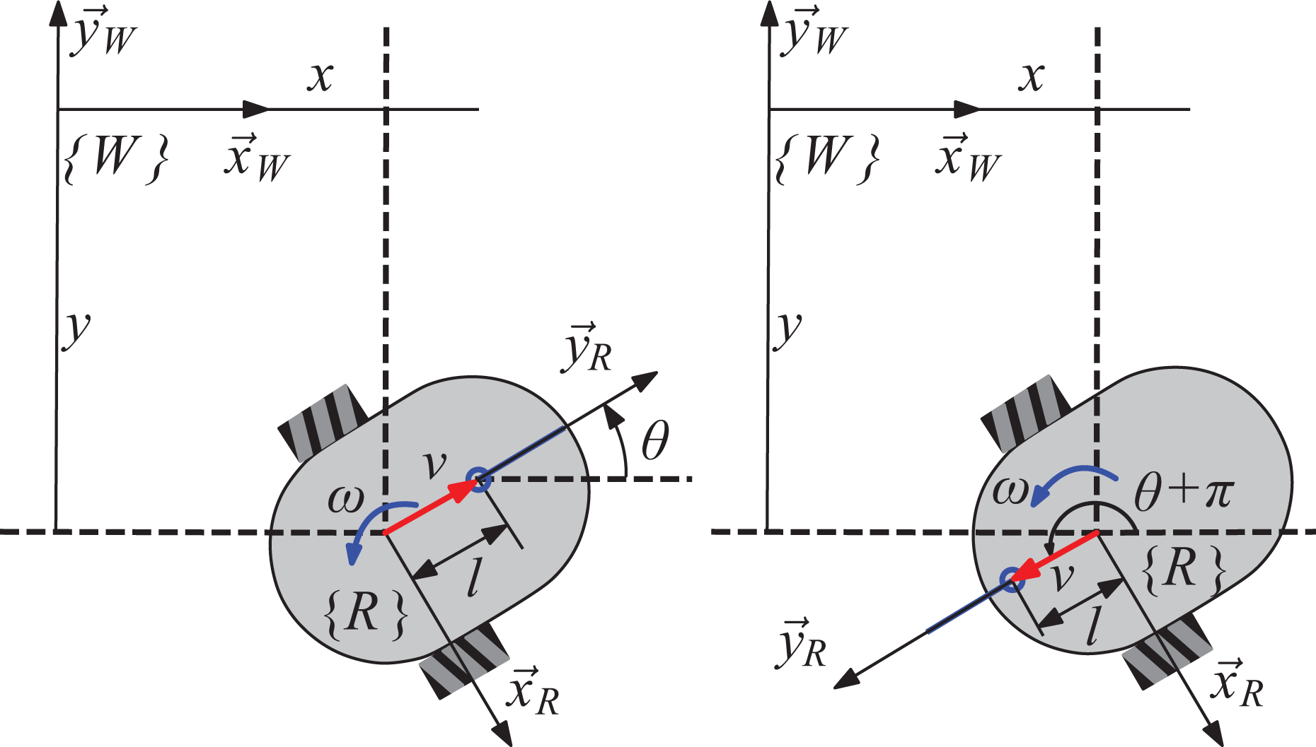
Kinematic configuration of the robot with a virtual control point at a distance l from the robot’s reference frame. Left: Forward motion model. Right: Backward motion model.

A transformed kinematic model

In this section, we modify the system (1) via the addition of a virtual point at a distance l along the longitudinal axis of the robot (see Figure 1). Hence, the well-defined change of coordinates

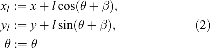
\begin{array}{l} x_{l} : = x + l cos (θ + β), \\ y_{l} : = y + l sin (θ + β), \\ θ : = θ \end{array}

with l > 0 and constant, transforms (1) into

[\begin{array}{l} {\dot{x}}_{l} \\ {\dot{y}}_{l} \\ \dot{θ} \end{array}] = [\begin{array}{l} cos (θ + β) & - l sin (θ + β) \\ sin (θ + β) & l cos (θ + β) \\ 0 & 1 \end{array}] (u + d)

For the controller design and to simplify the notation, we partition and recalled the coordinates as

z = col (x_{l}, y_{l}) \in ℝ^{2}

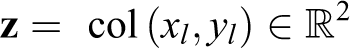
such that the modified model (3) can be written as

\begin{array}{l} \dot{z} : = A (θ + β) (u + d), \\ \dot{θ} : = ω + d_{2} \end{array}

with full rank matrix $A (θ + β)$ : ℝ → $\in ℝ^{2 \times 2}$ given by

A (θ + β) : = A = [\begin{array}{l} cos (θ + β) & - l sin (θ + β) \\ sin (θ + β) & l cos (θ + β) \end{array}]

Problem formulation

Consider the perturbed kinematic model (1), transformed to system (4) by the change of coordinates (2). The robust pose-regulation problem in a desired time can be enunciated as follows.

Definition 2.1

Problem statement. Regulate z and θ of the system (4) to desired constant values $z^{f} = col (z_{1}^{f}, z_{2}^{f}) \in ℝ^{2}$ and θ^f in a user-defined time τ in spite of the disturbance d. Without loss of generality, we will assume $z^{f} = 0$ .

In order to deal with the time-constraint imposed by τ, we propose to address the regulation problem as a trajectory tracking problem for adequate references of the position coordinates x_l and y_l. We will show that by tracking some particular trajectories, the orientation θ can also reach a desired value since the robot’s heading evolves tangent to the trajectory of position. By assuming that $z^{f} = 0$ , we consider that the robot’s desired final position will be the origin of ℝ².

Robust trajectory tracking control

In this section, we present a main result of the article, specifically two feasible controllers are described to achieve trajectory tracking on coordinates related to the Cartesian position of the robot.

Definition 3.1

Control objective. Let us define a vector of tracking errors as

$\tilde{z} (t) : = z (t) - z^{d} (t) : = [\begin{array}{l} x_{l} (t) - x_{l}^{d} (t) \\ y_{l} (t) - y_{l}^{d} (t) \end{array}]$
6

with $x_{l}^{d}, y_{l}^{d}$ ∈ ℝ desired trajectories. The objective is to ensure ${lim}_{t \to \infty} \tilde{z} = 0$ to achieve trajectory tracking.

In order to reach the origin of ℝ² in the time τ as robot’s final position, we assume in the sequel that $z^{d} (t) = z^{f} = 0$ for t ≥ τ.

A first controller that achieves the previous control objective makes use of the well-known addition of integral action on actuated coordinates²⁷ in order to reject the disturbance d and it is presented in the following proposition.

Proposition 3.2

Consider the time derivative of (6) and (4) in closed-loop with the controller

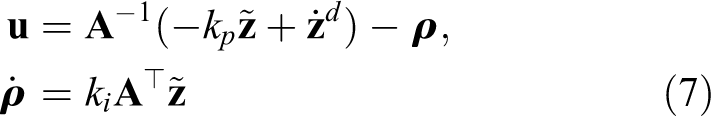
$u = A^{- 1} (- k_{p} \tilde{z} + {\dot{z}}^{d}) - ρ, \dot{ρ} = k_{i} A^{⊤} \tilde{z}$
7

with positive free gains $k_{p}, k_{i}$ and $ρ \in ℝ^{2}$ an integral action.

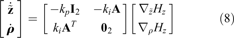
1. The closed-loop takes the form

$[\begin{array}{l} \dot{\tilde{z}} \\ \dot{ρ} \end{array}] = [\begin{array}{l} - k_{p} I_{2} & - k_{i} A \\ k_{i} A^{Τ} & 0_{2} \end{array}] [\begin{array}{l} \nabla_{\tilde{z}} H_{z} \\ \nabla_{ρ} H_{z} \end{array}]$
8

with total energy function $H_{z} : ℝ^{2} \times ℝ^{2} \to ℝ$

$H_{z} (\tilde{z}, \tilde{ρ}) = \frac{1}{2} | \tilde{z} |^{2} + \frac{1}{2} k_{i}^{- 1} | \tilde{ρ} |^{2}$
9

where $\tilde{ρ} = ρ - d$ . Assuming that in this case d is a constant vector, we have $\dot{\tilde{ρ}} = \dot{ρ}$ .

2. The closed-loop system has a globally asymptotically stable equilibrium point at the desired point $(\tilde{z}, ρ) = (0, d)$ .

3. The closed-loop system has a zero dynamics²⁸ of first order given by

$\dot{θ} = - \frac{1}{l} (v_{1} sin θ - v_{2} cos θ) - ρ_{2} + d_{2} = 0$
10

where $v_{1} = - k_{p} {\tilde{z}}_{1} + {\dot{z}}_{1}^{d}$ and $v_{2} = - k_{p} {\tilde{z}}_{2} + {\dot{z}}_{2}^{d}$ .

Proof

Regarding to point 1, replacing the control law (7) in (4), we obtain the first row of the closed-loop system (8). The second row of (8) corresponds to the definition of the integral part given by (7). On the other hand, taking as Lyapunov function (9) and its time derivative along the system (8) yields

${\dot{H}}_{z} (\tilde{z}, \tilde{ρ}) = - k_{p} | \tilde{z} |^{2}$
11

This proves that $(0, d)$ is a stable equilibrium of the closed loop system (8). Furthermore, from (8) and knowing that $\tilde{z} = 0$ and ${\dot{H}}_{z} = 0$ , we have that $- A \tilde{ρ} = 0$ and $\dot{ρ} = 0$ . Hence, from the fact that $A$ is a full rank matrix, we can conclude that the trajectories of (8) will converge to the invariant set

$M = {(\tilde{z}, \tilde{ρ}) | \tilde{z} = 0, ρ = d} .$

This proves that the equilibrium point $(0, d)$ of the target dynamics (8) is asymptotically stable as stated in point 2. Finally, related to point 3, the closed-loop system reaches its zero dynamics ²⁸ when $z = z^{d} (t) = z^{f} = 0$ for t ≥ τ. Thus, the outputs z₁ and z₂ can be regulated to zero, but in system (4), the dynamics of orientation is remaining. Equation (10) is obtained from (7) noting that ω is the second component of the input’s vector u. Since v₁ = 0, v₂ = 0, and ρ = d when z₁ ≡ 0 and z₂ ≡ 0, the zero dynamics (10) represents a stable dynamics with bounded constant solution $\bar{θ}$ .

Hence, in the case of the system (4) with outputs $z_{1} = x_{l}$ , $z_{2} = y_{l}$ , the subset of the state space describing the zero dynamics is given by

$\begin{array}{l} Z^{} = {{[x_{l}, y_{l}, θ]}^{⊤} | z_{1} \equiv 0, z_{2} \equiv 0} \\ = {{[0, 0, \bar{θ}]}^{⊤}, \bar{θ} \in ℝ} \end{array}$

Zero dynamics in this control system means that when the variables related to the robot’s position are corrected, the orientation might be different to zero.

Remark 3.3

The addition of integral action on actuated coordinates presented in proposition 3.2 can be equivalent to add an integrator around the passive output for port-Hamiltonian systems,²⁷ where the task preserves stability in the presence of constant disturbances or modeling errors.

The following proposition presents a second option of robust controller to achieve the control objective of definition 3.1. It is based on continuous second-order sliding-mode control.

Proposition 3.4

Consider the time derivative of (6) and (4) in closed-loop with a super-twisting control

$u = A^{- 1} (- k_{1} S sign (\tilde{z}) + {\dot{z}}^{d} + σ), \dot{σ} = - k_{2} sign (\tilde{z})$
12

with $S = [\begin{array}{l} | {\tilde{z}}_{1} |^{1 / 2} & 0 \\ 0 & | {\tilde{z}}_{2} |^{1 / 2} \end{array}]$ and positive free gains $k_{1}, k_{2}$ .

1. The closed-loop system takes the form

$\dot{\tilde{z}} = - k_{1} S sign (\tilde{z}) + σ + ϱ, \dot{σ} = - k_{2} sign (\tilde{z})$
13

with $\dot{\tilde{z}} ϱ = A d$ a bounded disturbance.

2. The closed-loop system has a globally finite-time stable equilibrium point at the desired point $(\tilde{z}, σ) = (0, - ϱ)$ .

3. The closed-loop system has a zero dynamics of first order given by

$\dot{θ} = - \frac{1}{l} (v_{1} sin θ - v_{2} cos θ) + σ_{2} + ϱ_{2} = 0$
14

where $v_{1} = - k_{1} | {\tilde{z}}_{1} |^{1 / 2} s i g n ({\tilde{z}}_{1}) + {\dot{z}}_{1}^{d}$ and $v_{2} = - k_{1} | {\tilde{z}}_{2} |^{1 / 2} s i g n ({\tilde{z}}_{2}) + {\dot{z}}_{2}^{d}$ .

Proof

The point I can be directly verified by replacing the control law (12) in (4) to obtain the closed-loop system in (13). Notice that (13) expresses decoupled dynamics for ${\tilde{z}}_{1}$ and ${\tilde{z}}_{2}$ . Thus, the decoupled closed-loop dynamics using the change of variable $ξ_{i} = σ_{i} + ϱ_{i}$ can be expressed as

$\begin{array}{l} {\dot{\tilde{z}}}_{i} = - k_{1} | {\tilde{z}}_{i} |^{1 / 2} sign ({\tilde{z}}_{i}) + ξ_{i}, \\ {\dot{ξ}}_{i} = - k_{2} sign ({\tilde{z}}_{i}) + {\dot{ϱ}}_{i} \end{array}$
15

for i = 1, 2. Thus, related to point 2, it has been proved that, for bounded continuously differentiable disturbances, that is, if $| ϱ_{i} | < L$ and $| {\dot{ϱ}}_{i} | < M$ for some constants $L > 0, M > 0$ , the second-order systems (15) converge globally to the origin (z_i* = 0, ξ_i = 0) in finite-time if adequate positive control gains k₁ and k₂ are used.²⁹ Since ξ_i = 0, then we have $ϱ = - σ$ . Hence, all the trajectories of (13) will converge to the invariant set

$M = {(\tilde{z}, σ) | \tilde{z} = 0, σ = - ϱ}$

Finally, regarding to point 3, the derivation of the zero dynamics can be addressed similarly as in proposition 3.2. Since v₁ = 0, v₂ = 0, and $σ = - ϱ$ when $z_{1} \equiv 0$ and $z_{2} \equiv 0$ , the zero dynamics (14) represents a stable dynamics with bounded constant solution $\bar{θ}$ .

Remark 3.5

Both controllers given by (7) and (12) can be implemented for forward and backward motion to track desired trajectories. Consider u₁ as the first component of the control vector u. Then, each type of motion control is obtained as follows:
Forward motion control: set β = 0 in (5) and $v = + u_{1}$ .

Backward motion control: set β = π in (5) and $v = - u_{1}$ .

Desired trajectories definition

The problem stated in definition 2.1 requires the robot to reach a desired position and orientation. Up to now, the presented controllers drive to zero the position coordinates $z_{1} = x_{l}$ and $z_{2} = y_{l}$ , but the orientation evolves freely as given by the zero dynamics. We propose to carry out an offline trajectory planning stage to define an adequate desired trajectory for the robot’s position in order to obtain also orientation correction. This is achieved since the robot’s heading is tangent to the trajectory of position for nonholonomic mobile robots. Let us define an initial robot’s pose given by $(z_{1}^{i}, z_{2}^{i}, θ^{i})$ and a final desired pose given by $(z_{1}^{f}, z_{2}^{f}, θ^{f})$ . First, we propose the use of quadratic (parabolic) trajectories since they are the simplest polynomials that can build a good trajectory accomplishing a constraint for the tangent of the curve at a desired point. However, we also generalize the trajectory planning to the use of cubic trajectories and we propose to select the adequate trajectory to be tracked among a set of candidates from quadratic and cubic curves.

Let us first formulate the generation of a parabolic trajectory that accomplishes the constraint that the slope of the curve at the final desired position $(z_{1}^{f}, z_{2}^{f})$ must be equal to $tan θ^{f}$ . A parabolic trajectory on the $z_{1} - z_{2}$ plane symmetric to an axis parallel to ${\vec{z}}_{1}$ has the form

$4 p (z_{1} - h) = (z_{2} - k)^{2}$
16

where p ∈ ℝ represents the constant distance between the vertex and the focus and h, k ∈ ℝ are the vertex coordinates of the parabola (see Figure 2).

Figure 2.
Parabolic desired trajectory symmetric to an axis parallel to ${\vec{z}}_{1}$ , whose tangent at the origin of the plane is equal to $tan (θ^{f})$ .

Without loss of generality, consider the final desired position $z_{1}^{d} (τ) = z_{1}^{f} = 0$ and $z_{2}^{d} (τ) = z_{2}^{f} = 0$ . Taking the derivative of (16) evaluated at the desired position and equating to the slope given by $tan θ^{f}$ at the desired position, we have

$\frac{d z_{2}}{d z_{1}} |_{(0, 0)} = \frac{- 2 p}{k} = tan θ^{f}$
17

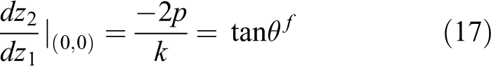
Moreover, evaluating (16) at the desired position (origin of the plane), we get

$k^{2} = - 4 p h$
18

Thus, from (17) and (18), the parameters h and k are give by

$h = \frac{- p}{{tan}^{2} θ^{f}}, k = \frac{- 2 p}{tan θ^{f}}$
19

Since we know the initial position $(z_{1}^{i}, z_{2}^{i})$ and solving for p in (16), we get $p = \frac{{(z_{2}^{i})}^{2}}{4 (z_{1}^{i} - \frac{z_{2}^{i}}{tan θ^{f}})}$

Then, using the previous results, the proposed trajectory is generalized for an initial pose $(z_{1}^{i}, z_{2}^{i}, θ^{i})$ and a final pose $(z_{1}^{f}, z_{2}^{f}, θ^{f})$ and parameterized in time as follows

$\begin{array}{l} z_{2}^{d} (t) = \frac{z_{2}^{i} - z_{2}^{f}}{2} (1 + cos (\frac{π t}{τ})) + z_{2}^{f}, 0 \leq t \leq τ \\ z_{1}^{d} (t) = {\frac{(z_{2}^{d} (t) - z_{2}^{f} - k)}{4 p}}^{2} + z_{1}^{f} + h, 0 \leq t \leq τ \\ p = \frac{{(z_{2}^{i} - z_{2}^{f})}^{2}}{4 (z_{1}^{i} - z_{1}^{f} - \frac{z_{2}^{i} - z_{2}^{f}}{tan θ^{f}})} \end{array}$
20

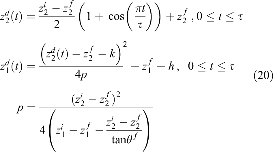
Notice that the computation of the parameters p, h, and k for the trajectory (20) has singularities for some values of θ^f (0° and 180°). Hence, we propose another complementary option of trajectory that can be used conveniently to avoid the singularities. Following a similar procedure to the previous one, we can define a parabolic trajectory on the $z_{1} - z_{2}$ plane symmetric to an axis parallel to ${\vec{z}}_{2}$ , which is given by (see Figure 3)

$4 p (z_{2} - k) = (z_{1} - h)^{2} .$
21

Figure 3.
Parabolic desired trajectory symmetric to an axis parallel to ${\vec{z}}_{2}$ , whose tangent at the origin of the plane is equal to $tan (θ^{f})$ .

By parameterization of equation (21) in time, we define the following complementary option of desired trajectory

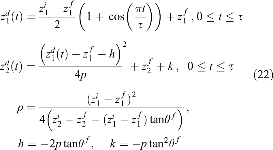
$\begin{array}{l} z_{1}^{d} (t) = \frac{z_{1}^{i} - z_{1}^{f}}{2} (1 + cos (\frac{π t}{τ})) + z_{1}^{f}, 0 \leq t \leq τ \\ z_{2}^{d} (t) = {\frac{(z_{1}^{d} (t) - z_{1}^{f} - h)}{4 p}}^{2} + z_{2}^{f} + k, 0 \leq t \leq τ \\ p = \frac{{(z_{1}^{i} - z_{1}^{f})}^{2}}{4 (z_{2}^{i} - z_{2}^{f} - (z_{1}^{i} - z_{1}^{f}) tan θ^{f})}, \\ h = - 2 p tan θ^{f}, k = - p {tan}^{2} θ^{f} \end{array}$
22

Notice that this second option of trajectory also presents singularities for $θ^{f} = \pm 90 °$ , in which case the vertex of the parabola goes to infinity. In order to have more options of trajectories without singularities and looking for trajectories that favor the orientation correction, we propose to generalize the trajectory planning by formulating also cubic curves. These trajectories provide an additional degree of freedom that can improve the accuracy of the desired orientation correction as will be explained later. Let us formulate the generation of cubic trajectories accomplishing the constraint of the curve’s slope at the final position. Consider the following polynomial

$z_{2} = a_{0} + a_{1} z_{1} + a_{2} z_{1}^{2} + a_{3} z_{1}^{3}$
23

where $a_{0}, a_{1}, a_{2}$ and $a_{3} \in ℝ$ are constant coefficients. We can compute these coefficients by imposing the following constraints: $z_{1}^{f} = 0$ , $z_{2}^{f} (z_{1}^{f}) = 0$ , $z_{2}^{i} (z_{1}^{i}) = z_{2}^{i}$ , $\frac{d z_{2}}{d z_{1}} (z_{1}^{f}) = tan θ^{f}$ , $\frac{d z_{2}}{d z_{1}} (z_{1}^{i}) = tan ϕ^{i}$ , where $tan ϕ^{i}$ is a desired slope of the trajectory at the initial position and this slope will be used as a degree of freedom to obtain a set of candidate trajectories. For the cubic trajectories, we will assume that the final desired position is the origin of the plane ( $z_{1}^{f} = 0, z_{2}^{f} = 0$ ) to obtain short expressions for the coefficients; however, it can be generalized for any desired position. Evaluating the constraints in expression (23), we have

$\begin{array}{l} a_{0} = 0, \\ a_{1} = tan θ^{f}, \\ a_{2} = \frac{3 z_{2}^{i} - z_{1}^{i} (tan ϕ^{i} + 2 tan θ^{f})}{{(z_{1}^{i})}^{2}}, \\ a_{3} = \frac{z_{1}^{i} (tan ϕ^{i} + tan θ^{f}) - 2 z_{2}^{i}}{{(z_{1}^{i})}^{3}} \end{array}$
24

Thus, we define the following time-parameterized cubic trajectory

$\begin{array}{l} z_{1}^{d} (t) = \frac{z_{1}^{i}}{2} (1 + cos (\frac{π t}{τ})), 0 \leq t \leq τ \\ z_{2}^{d} (t) = a_{0} + a_{1} z_{1}^{d} + a_{2} {(z_{1}^{d})}^{2} + a_{3} {(z_{1}^{d})}^{3}, 0 \leq t \leq τ \end{array}$
25

Now consider the following complementary cubic polynomial

$z_{1} = a_{0} + a_{1} z_{2} + a_{2} z_{2}^{2} + a_{3} z_{2}^{3}$
26

The corresponding coefficients are computed by imposing the following constraints: $z_{2}^{f} = 0$ , $z_{1}^{f} (z_{2}^{f}) = 0$ , $z_{1}^{i} (z_{2}^{i}) = z_{1}^{i}$ , $\frac{d z_{1}}{d z_{2}} (z_{2}^{f}) = \frac{1}{tan θ^{f}}$ , and $\frac{d z_{1}}{d z_{2}} (z_{2}^{i}) = \frac{1}{tan ϕ^{i}}$ , where $tan ϕ^{i}$ is a desired slope of the trajectory at the initial position. Evaluating the constraints in expression (26), we have

$\begin{array}{l} a_{0} = 0, \\ a_{1} = \frac{1}{tan θ^{f}}, \\ a_{2} = \frac{3 z_{1}^{i} - z_{2}^{i} (\frac{1}{tan ϕ^{i}} + \frac{2}{tan θ^{f}})}{{(z_{2}^{i})}^{2}}, \\ a_{3} = \frac{z_{2}^{i} (\frac{1}{tan ϕ^{i}} + \frac{1}{tan θ^{f}}) - 2 z_{1}^{i}}{{(z_{2}^{i})}^{3}} \end{array}$
27

Thus, we define the complementary option of time-parameterized cubic trajectory as

$\begin{array}{l} z_{2}^{d} (t) = \frac{z_{2}^{i}}{2} (1 + cos (\frac{π t}{τ})), 0 \leq t \leq τ \\ z_{1}^{d} (t) = a_{0} + a_{1} z_{2}^{d} + a_{2} {(z_{2}^{d})}^{2} + a_{3} {(z_{2}^{d})}^{3}, 0 \leq t \leq τ \end{array}$
28

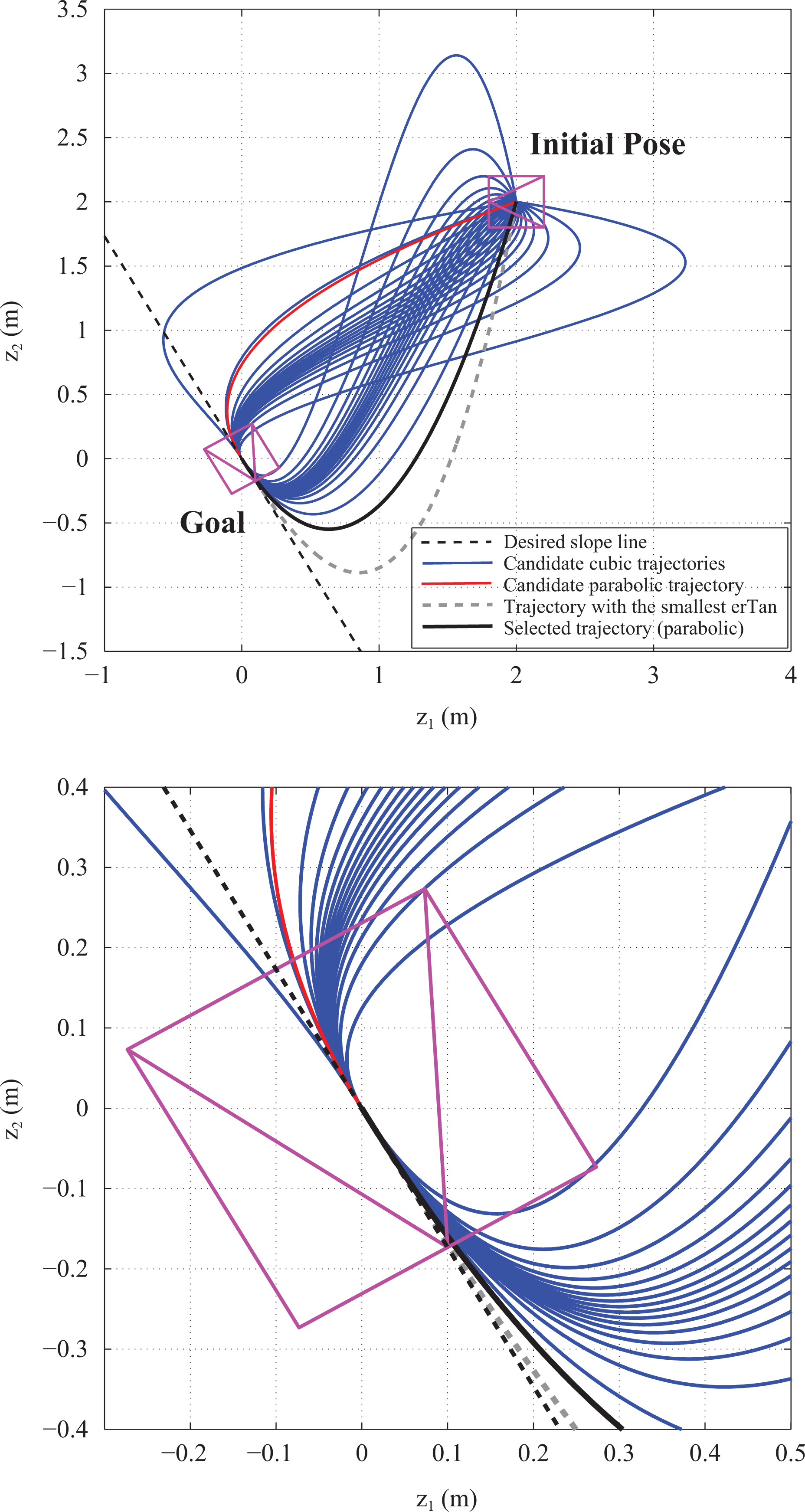
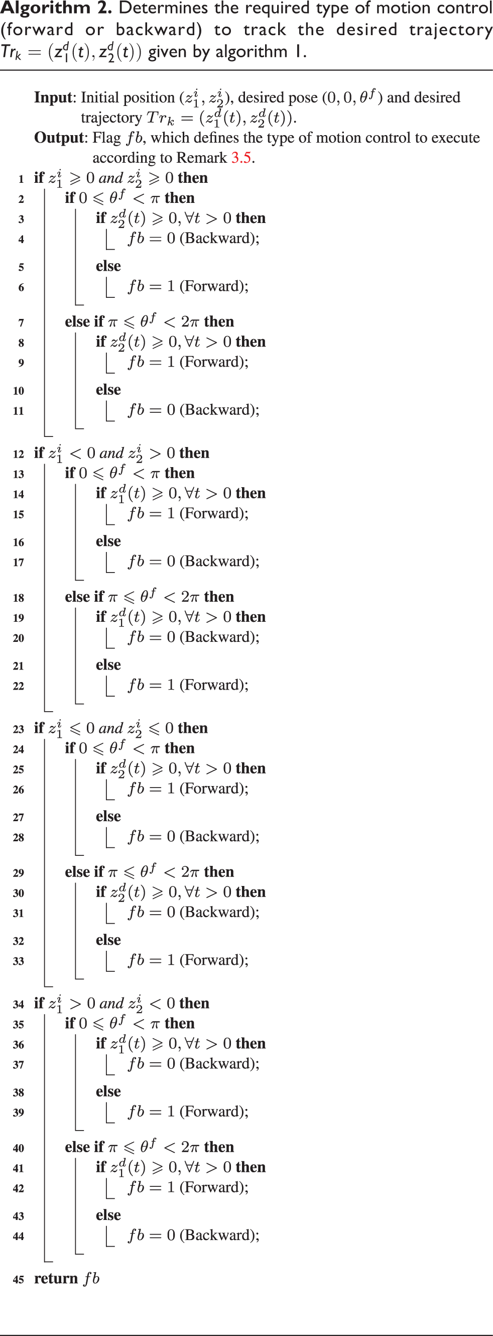
Notice that the computation of coefficients (24) and (27) also generates singularities for some values of θ^f and ϕⁱ; however, we can have many options of trajectories to chose a non-singular one. Actually, we can generate a set of candidate trajectories and we have two ways of motion control to track the selected trajectory (forward and backward). The candidates are the result of the two parabolic trajectories of (20) and (22) and the two cubic trajectories (25) and (28) for different values of the degree of freedom ϕⁱ involved in the coefficients of the polynomials. Thus, we propose a strategy to select the trajectory which favors the accuracy to reach the desired orientation. Algorithm 1 presents our proposal to generate a set of candidate trajectories, all of them reaching the desired position and accomplishing the constraint of the curve’s slope at the final position. From a set of candidate parabolic and cubic trajectories, the notion is to select the trajectory whose error between its slope and the desired slope ( $tan θ^{f}$ ) at some time before ( $t = 0.95 τ$ ) to reach the desired position is the minimum and whose length is reasonable (not more than 1.5 times the distance from the initial position to the desired one).

Algorithm 1
Generates a set of candidate trajectories and finds the best one to be tracked.

Figure 4 shows an example of the execution of algorithm 1 for some initial and desired poses. The desired final slope is depicted as the dashed black line. The red curve corresponds to one of the parabolic candidate trajectories. The set of blue curves are generated by the cubic polynomials using ϕⁱ from 0° to 180° with increments of δ = 10°. Thus, we have a total of n = 40 candidate trajectories. From those trajectories, the one whose slope is closest to the desired one some time before to reach the final position is the dashed gray line. Such trajectory favors the accuracy to reach the desired orientation due to the robot aligns to the desired orientation previous to reach the desired position, preventing to perform large rotations at the end that might introduce orientation error. Usually, trajectories that best favor the orientation correction are long trajectories and the selection must be constrained to a reasonable length. In the case of the figure, the finally selected trajectory is shown as a continuous black line and corresponds to a parabolic curve. It provides a good compromise between orientation correction and length of the trajectory. Of course, it is not always the case that a parabolic trajectory is selected.

Figure 4.
Different candidate trajectories to reach the pose ( $z_{1}^{f} = 0$ , $z_{2}^{f} = 0$ , $θ^{f} = 300 °$ ) from ( $z_{1}^{i} = 2$ , $z_{2}^{i} = 2$ , $θ^{i} = 180 °$ ). Top: All candidate trajectories and the selected one are shown. Bottom: Details close to the desired position.

As aforementioned, singularities in the computation of candidate trajectories appear for some values of θ^f and ϕⁱ. However, for general initial and desired poses, many candidate trajectories can be generated from the non-singular values and one trajectory can be selected. Some particular poses are an issue for the proposed strategy, where no feasible candidate trajectories of limited length can be generated, for example, when $z_{1}^{i} \neq 0, z_{2}^{i} = 0$ , and $θ^{f} = \pm 90 °$ . Those cases are detectable and the robot might be moved away from that condition (for instance by moving forward during a short time). Then, starting from a general pose, the proposed strategy of algorithm 1 can be applied.

To finish the description of the planning stage that defines the desired trajectory, notice in Figure 4 that the selected trajectory must be tracked in backward motion to reach the desired orientation $θ^{f} = 300 °$ , otherwise, the final orientation will be $θ^{f} = 120 °$ . Then, once the best candidate trajectory is selected, a decision about the type of motion control must be taken. Algorithm 2 presents an empirical strategy to decide the type of motion control that exhaustively considers any situation of initial pose and desired orientation. The algorithm returns a flag (fb) that specifies the direction of motion to be executed. According to that flag, the parameter β and the sign of u₁ (the first component of the computed control vector) must be set according to remark 3.5. It is worth emphasizing that the selection of the desired trajectory and the decision of direction of motion are carried out offline, previous to the autonomous robot motion. Once this planning stage is done, a control stage is performed to achieve the pose-regulation task.

Algorithm 2
Determines the required type of motion control (forward or backward) to track the desired trajectory $T r_{k} = (z_{1}^{d} (t), z_{2}^{d} (t))$ given by algorithm 1.

The tracking of the proposed trajectories allow us to define a fixed temporal horizon τ to reach the desired robot pose at difference of classical stabilization/regulation schemes for WMR.^5,2 Notice that the robot always begins over the desired trajectory, so that the controller has to maintain the tracking of it. Due to the nonholonomic motion of the robot, the tracking controller drives the robot to perform an initial autonomous rotation to get aligned with the trajectory, independently of the initial robot orientation. Next, it is proved that the desired orientation is also achieved by tracking the proposed trajectories, in such a way that pose-regulation is accomplished.

Proposition 4.1

The tracking of the reference trajectory specified by algorithm 1 using any of the robust controllers (7) or (12) and the type of motion determined by algorithm 2 drives the virtual control point of the perturbed differential-drive robot (4) to reach the desired pose ( $z_{1} = 0, z_{2} = 0$ and $θ + β = θ^{f}$ without loss of generality), that is, orientation is also corrected, in τ seconds.

Proof

It is clear the global robust stability of the error system (8), respectively (13), with the controller (7), respectively (12), which drives the robot position to the desired values $(z_{1} = 0$ , $z_{2} = 0)$ in τ seconds. Thus, it remains to prove that the orientation is also corrected in τ seconds. We assume that the rotational velocity is small when the robot is approaching to the desired position, which is realistic given the construction of the desired trajectory. Thus, the translational velocities of the virtual control point for each axis are given by

${\dot{z}}_{1} = v cos (θ + β), {\dot{z}}_{2} = v sin (θ + β)$

From these relationships we get

$tan (θ + β) = \frac{{\dot{z}}_{2}}{{\dot{z}}_{1}} = \frac{d z_{2}}{d z_{1}}$
29

Let us consider the relationships between Cartesian coordinates of the parabolic trajectory (22) and the cubic trajectory (25) as instances of our procedure. A similar analysis follows for the complementary trajectories (20) and (28). The derivative $\frac{d z_{2}}{d z_{1}}$ of (22) or (25) provides the relationships

$\frac{d z_{2}}{d z_{1}} = \frac{z_{1} - h}{2 p}, \frac{d z_{2}}{d z_{1}} = tan θ^{f} + 2 a_{2} z_{1} + 3 a_{3} z_{1}^{2}$

for the parabolic and cubic trajectories, respectively. Thus, according to (29), the robot’s orientation can be computed as follows when the z₁ and z₂-coordinates track the corresponding desired trajectory for the parabolic and cubic trajectories, respectively

$\begin{array}{l} θ + β = arctan (\frac{z_{1} - h}{2 p}), \\ θ + β = arctan (tan θ^{f} + 2 a_{2} z_{1} + 3 a_{3} z_{1}^{2}) \end{array}$
30

As aforementioned, when the robot has tracked the corresponding trajectory and t = τ, the position reaches the goal (z₁ = 0, z₂ = 0). Since the trajectories are defined such that their slope comply with the constraint $\frac{d z_{2}}{d z_{1}} (z_{1} = 0) = tan θ^{f}$ , we have

$θ + β = arctan (- \frac{h}{2 p}) = θ^{f}$
31

for the parabolic trajectory according to the equation of h in (22). It directly follows from (31) that $θ + β = θ^{f}$ for the cubic trajectory (25). This proves that the desired pose $(z_{1} = 0$ , z₂ = 0, and $θ + β = θ^{f})$ is reached in τ seconds.

Evaluation of the method

In this section, we present an evaluation of the proposed method through simulations and experiments using indistinctly each controller, (7) the proportional–integral control (PIC) or (12) the super-twisting control (STC). Simulations were implemented using Webots³⁰ with the differential-drive robot Pioneer 3-DX [Figure 5 (left)]. A GPS and a compass provide the required feedback information. Experiments were carried out using a TurtleBot 2 robot (Figure 5 (right)). A motion capture system provides the position and orientation of the robot for feedback. The time-derivatives required by the control laws are implemented using the forward Euler approximation. It is worth noting that the method can be applied using any differential-drive robot, the robots used in the evaluation of the method, the Pioneer 3-DX and the TurtleBot 2, are just two examples.
Figure 5.
Experimental setup using Webots simulator17 with a Pioneer 3-DX robot (left) and using a real robot TurtleBot 2 (right).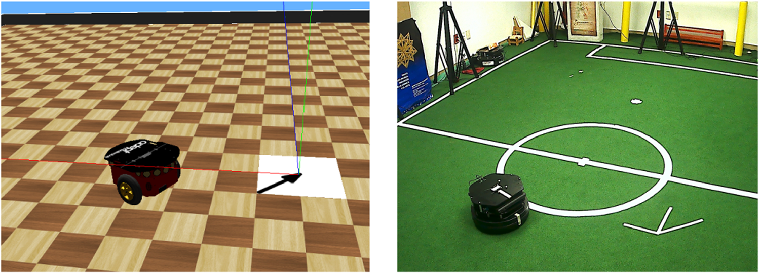

Simulation results

First, we present simulation results obtained in Webots. In all the simulations, we have introduced as disturbances d₁ = 0.1 m/s for the translational velocity v and d₂ = −0.1 rad/s for the rotational velocity ω. We assumed that the virtual control point is at l = 0.1 m. The control gains were fixed to k_p = 1.5, k_i = 1.5 for the PIC and k₁ = 0.6, k₂ = 0.03 for the STC. As shown in “Robust trajectory tracking control” section, the stability of the closed-loop dynamics is verified for positive control gains; however, it is expected that the reference tracking performance degenerates for small control gains. Thus, the gains were manually tuned to obtain small tracking errors. Notice that the tracking errors start in zero because the virtual control point starts on the reference trajectory, the controller must keep the errors around zero and therefore no high gains are needed.

We have defined that the robot has to reach the desired pose in τ = 30 s in most of the simulations. An important consideration for the parameter τ is that it must not be too small such that the maximum translational robot speed v^max could be exceeded for the desired traverse distance. For the Pioneer 3-DX robot, $v^{max} = 1.2$ m/s. The simulated control cycle runs at 5 ms, which is enough to achieve a good behavior of the STC that works better for high control rates.^13,29 We use a parameter δ = 5° in algorithm 1 in order to generate candidate trajectories with different initial slopes.

Comparison with other approaches

In this first part of the results, we compare the proposed approach with two existing methods in the literature for simultaneous convergence of position and orientation of differential-drive robots. The first method, proposed by Martins et al.,¹² is similar to ours in the sense that it is a robust trajectory tracking scheme for wheeled robots able to reject kinematic disturbances. In that work, the kinematic controller is formulated using the classical idea of a virtual reference robot^5,6,14 with a discontinuous sliding-mode control. It is the kind of scheme that controls the three state variables of the robot to track desired values. The second method to compare, proposed by López-Nicolás and Sagüés,¹¹ is a different approach that provides exponential stabilization of the robot state, such that the executed trajectories are arbitrary. For the Martins’ scheme, we use the same trajectories than ours with the same magnitude of disturbance of 0.1, while for the López-Nicolás’ scheme, we introduce a very small disturbance a thousand times smaller, since it is not a robust approach. We report the results using the PIC; however, similar results are obtained with the STC.

Figure 6 shows the results for each one of the compared schemes initializing the robot from 10 different poses. In all the cases, the desired position is the origin of the plane and the desired orientation is zero. From the 10 initial poses, we have included in the plots the best and worst final pose of the robot in terms of position and orientation errors. The best case is shown in black and the worst case in red. Although the three schemes are able to drive the robot to a neighborhood of the desired pose, the proposed approach behaves better than the other two, being very accurate in the best case and with a reasonable orientation error in the worst case. The quantitative information of the final error is given in Table 1. For all the three schemes, the best case corresponds to the initial poses where the robot moves in straight line to reach the goal and the worst case corresponds to the initial poses where the robot has to perform a large rotation close to the goal.

Figure 6.
Comparison of control schemes for simultaneous convergence of position and orientation from different initial positions. Top-left: the proposed approach using the PIC. Top-right: Martins et al. scheme.¹⁶ Bottom: López-Nicolás and Sagüés’ scheme.¹¹ PIC: proportional–integral control; STC: super-twisting control.

Table 1.
Comparison of control schemes for simultaneous convergence of position and orientation for the best and worst experimental runs presented in Figure 6.

Proposed PIC Martins et al.¹² López-Nicolás and Sagüés¹¹

Final errors Best Worst Best Worst Best Worst

Orientation (degree) <1 −4.58 <1 5.16 <1 26.55

Position (cm) <1 <1 <1 8.37 <1 <1

PIC: proportional–integral control.

Different final orientations from the same initial pose

The second part of the results evaluates the proposed approach for a single initial robot pose (x = 3 m, y = 2 m, θ = 180°) to reach the origin of the z₁ − z₂ plane for four experimental runs and for a different final desired orientation in each case. The desired orientation for each case is $θ^{f} = 0 °$ , $θ^{f} = 150 °$ , $θ^{f} = 220 °$ , and $θ^{f} = 315 °$ . Figure 7 depicts the execution of algorithm 1 for the case of desired orientation $θ^{f} = 0 °$ . The best option of trajectory according to that algorithm is the cubic trajectory shown in black. This is due to such curve better approaches to the horizontal slope before the goal point. Once the trajectory is selected, algorithm 2 determines in lines 1 − 4 that it must be tracked in backward motion. A common approach in robotics for trajectory generation is the use of Bezier curves^24,25 or splines in general, which assumes that the departure angle of the trajectory is equal to the initial orientation of the robot. Notice that in the proposed trajectory generation, one of the candidates may correspond to such spline. In Figure 7, we have a candidate trajectory with horizontal initial slope (as the initial robot orientation); however, such trajectory is not selected as the best to favor the final orientation correction. This is recurrent for different initial poses and justifies the need of using a set of candidate trajectories and a selection algorithm instead of a single spline.

Figure 7.
Different candidate trajectories according to algorithm 1 for initial robot pose $P = (x = 3$ m, y = 2 m, θ = 180°) to reach the origin of the plane with desired orientation θ^f = 0°.

Figure 8 shows the executed trajectories and the corresponding references for the four experimental runs. Two of the cases were executed using the PIC and the other two using the STC. In the four cases, the desired trajectories were selected as cubic curves by algorithm 1. The trajectory to reach θ^f = 0° is the only one tracked in backward motion and the others are tracked in forward motion according to algorithm 2. This is why the trajectory in black in Figure 8, corresponding to θ^f = 0, starts in a different position than the others, since the virtual control point in this case is behind the robot reference frame as defined in Figure 1 (right). For each of the evaluated cases in Figure 8, the final position error, given by the Euclidean distance between the final position and the origin of the plane, is less than 1 cm for each case. The mean squared tracking error is less than 10 cm² for each case. The final orientation errors for the goals θ^f = 0 deg, θ^f = 150°, θ^f = 220°, and θ^f = 315° are 0.8 deg, 4.9 deg, 0.4 deg, and 2.3 deg, respectively.

Figure 8.
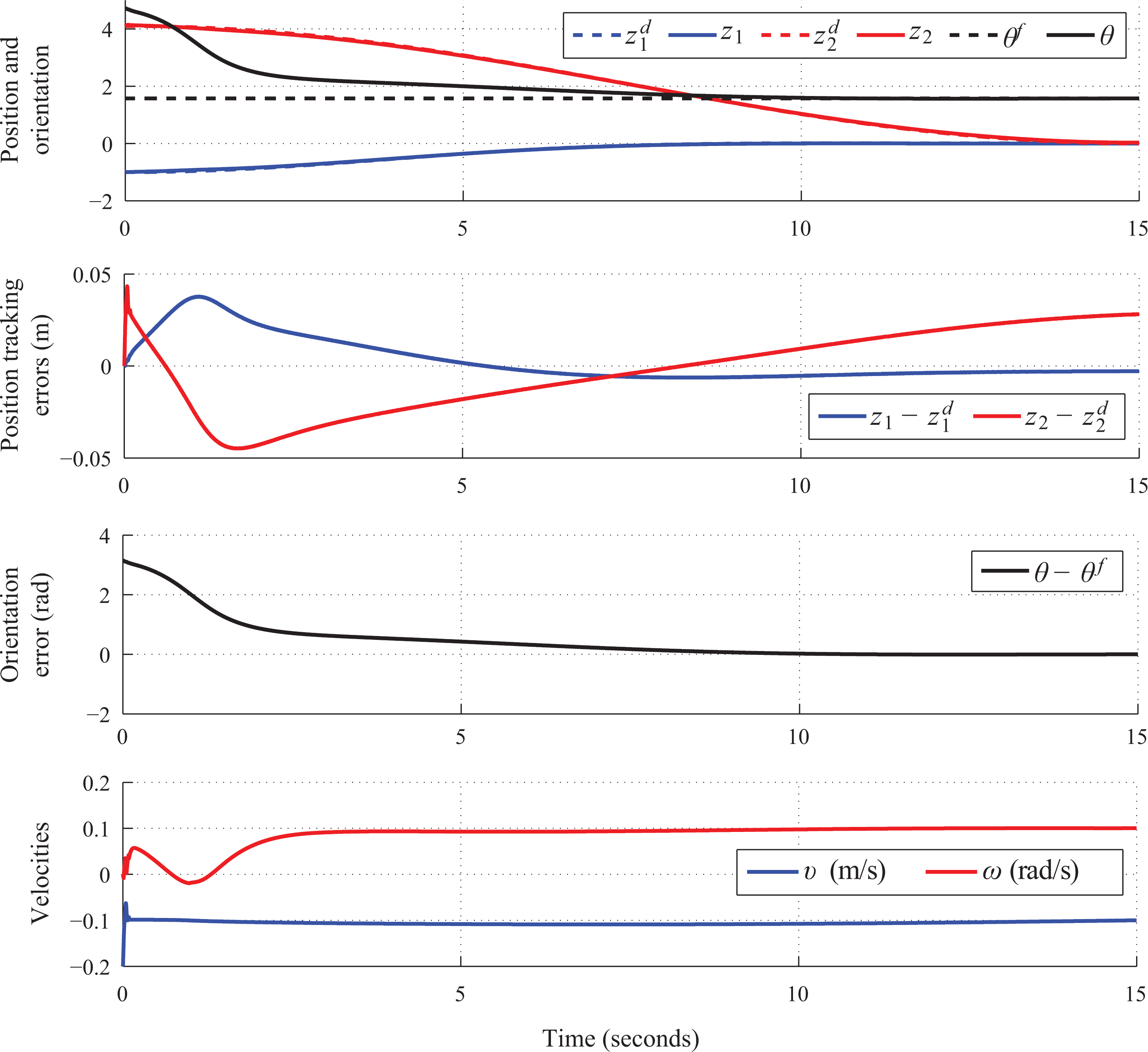
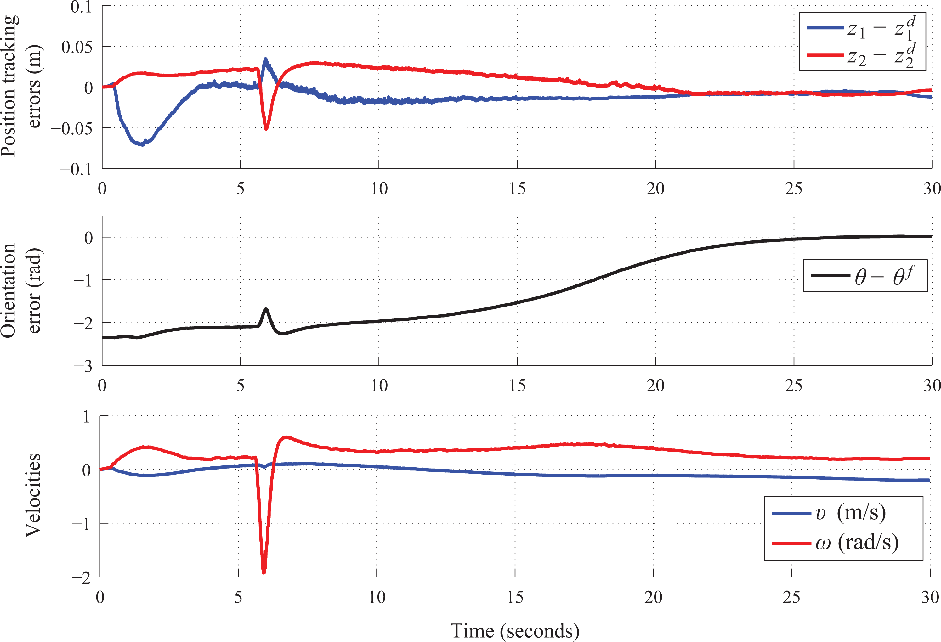
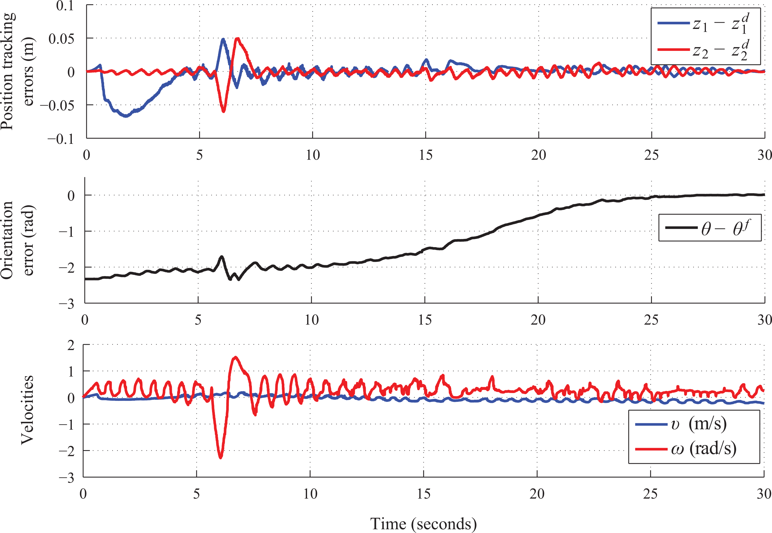
Executed and desired trajectories starting from the same initial robot pose $P = (x = 3$ m, y = 2 m, θ = 180°) and reaching the origin of the plane with four different desired orientations in 30 s. PIC: proportional–integral control; STC: super-twisting control.

Two examples, for θ^f = 0° with STC and θ^f = 220° with PIC, of the evolution of the robot pose, errors, and velocities with respect to time are shown in Figures 9 and 10, respectively. We can see the good tracking of the desired trajectories for position coordinates z₁ and z₂, such that the real evolution of these variables are almost over imposed to the references. Also, the orientation error is taken really close to zero in the desired time τ = 30 s using either controller. The bottom plots of the same Figures 9 and 10 present the evolution of the robot velocities with respect to time. A transient response can be appreciated in the plots of the rotational velocity in the first 5 s. This is due to the initial rotation that the controller enforces on the robot to align it to the trajectory. The transient could be faster for higher control gains, but the magnitude of the required velocities would increase up the maximum allowable range, which is not desirable. Currently, we left as future work to consider velocity constraints in the design of trajectories and gains tuning. According to the figures, the velocities settle at the contrary sign values of the introduced constant disturbances, such that they are effectively rejected. Notice that although the STC is continuous in contrast to classical sliding mode control,²⁹ it generates a small high-frequency component on the velocities that can be reduced if the control loop is even faster.

Figure 9.
Evolution of the robot pose, errors, and velocities with respect to time for the case of desired orientation θ^f = 0° using the STC. STC: super-twisting control.

Figure 10.
Evolution of the robot pose, errors, and velocities with respect to time for the case of desired orientation θ^f = 220 deg using the PIC. PIC: proportional–integral control.

We present a set of snapshots of the simulated experiment for the case of desired orientation θ^f = 315° in Figure 11. The top-left image corresponds to the initial pose and the bottom-right corresponds to the final pose. It can be seen that the robot moves forward in this case. The goal pose is reached in the desired time considering the capture time of the snapshots (see Figure 11).

Figure 11.
Snapshots of an experiment at t = 0, 2, 6, 10, 14, 18, 22, 26, and 30 s for the case of desired orientation θ^f = 315° using the STC. The arrow on the floor indicates the desired final position (arrowhead) and orientation. STC: super-twisting control

A single final pose from different initial poses

The third part of the results corresponds to four different initial robot poses to reach the origin of the z₁ − z₂ plane with desired orientation θ^f = 90° deg for all the cases. Additionally, we tested the behavior of the method for a higher robot speed, that is, the desired time to reach the target was reduced in the middle (now 15 s). As expected, if the robot is required to reach the target faster (of course complying with the velocity bounds), a faster correction of the tracking errors is needed to maintain a good performance, and consequently the control gains must be higher. Thus, the control gains were changed two times larger than in the previous simulations and the speed of the control cycle was reduced to 1 ms. Figure 12 presents the executed trajectories and the corresponding references for each experimental run. Two of the cases were executed using the PIC and the other two using the STC. In this second part, algorithm 1 determines that for the case of initial pose P₃ the reference trajectory is parabolic, while for the others are cubic curves. Moreover, the strategy of algorithm 2 specifies that the trajectories starting in P₁ and P₂ are executed in backward motion and those starting in P₃ and P₄ are executed in forward motion. Similar performance to the first part of the results was obtained in this second part. For each of the cases in Figure 12, the final position error is less than 1 cm and the mean squared tracking error is less than 10 cm². The final orientation errors are −1.4° for P₁, 0.1° for P₂, −7.1° for P₃, and −8.1° for P₄.

Figure 12.
Executed and desired trajectories starting from four different initial robot poses $P_{1} = (x = 2$ m, y = 3 m, θ = 180°), $P_{2} = (x = - 1$ m, y = 4 m, θ = 270°), $P_{3} = (x = - 4.5$ m, y = −3 m, θ = 90°), and $P_{4} = (x = 2.5$ m, y = −2 m, θ = 90°) and reaching the origin of the plane with desired orientation 90° deg in 15 s.

Figures 13 and 14 show the evolution of the robot pose, errors, and velocities with respect to time for the cases starting in P₂ and P₃. The real evolution of the position coordinates z₁ and z₂ are practically over imposed to the references, which demonstrates the good performance of both tracking controllers. Also, the robot orientation closely reaches the desired value in the specified time τ = 15 s. Regarding to the robot velocities shown at the bottom plots of Figures 13 and 14, it can be seen that the settling values are those that effectively cancel the introduced disturbances. In Figure 15, we present snapshots of the simulation for the case of initial pose P₂. It can be seen that an initial rotation is carried out by the robot (top line of snapshots) and then the robot moves backward to reach the goal position with the desired orientation in the specified time.

Figure 13.
Evolution of the robot pose, errors and velocities with respect to time for the case of initial pose P₂ using the PIC. PIC: proportional–integral control.

Figure 14.
Evolution of the robot pose, errors and velocities with respect to time for the case of initial pose P₃ using the STC. STC: super-twisting control.

Figure 15.
Snapshots of the simulation at t = 0, 1, 3, 5, 7, 9, 11, 13, and 15 s for the case of P₂ using the PIC. The arrow on the floor indicates the desired final position (arrowhead) and orientation. PIC: proportional–integral control.

Experiments with a real robot

We also evaluated the method using a real differential-drive robot, a TurtleBot 2, also considering more severe disturbances in the robot velocities and an external disturbance produced by pushing the robot. The push makes that the robot deviates from the desired trajectory for a while, but it recovers the trajectory to eventually reach the desired position and orientation in the desired time (see Figure 16). Notice that we could use any external disturbance that deviates the robot from the desired trajectory, the push by a person is just an example. Another example is a crash with an obstacle that deviates the robot. In this case, the disturbances of the velocities were increased to d₁ = 0.2 m/s for the translational velocity v and d₂ = −0.2 rad/s for the rotational velocity ω. It is important to notice that we have re-tuned the gains only for these experiments that include an external disturbance, since the deviation of the robot from the desired trajectory may generate large transient velocities. As we are not estimating the magnitude of the disturbance neither its effect in the tracking error, we cannot ensure that the velocities are below their bounds during the transient. In the cases without external disturbance, exceeding the velocity bounds is not a major concern since the tracking error starts in zero and the controller just must keep it low. For the experiments, the control gains were set to k_p = 1.5 and k_i = 1.5 for the PIC and k₁ = 0.57 and k₂ = 0.05 for the STC. These gains were defined experimentally to achieve a compromise between good disturbance rejection and final accuracy in the position and orientation correction without exceeding the velocity bounds. This multicriterion context makes the adjustment of the controller gains not an easy task, further knowing that in any control system the gains must be re-tuned for different operation conditions. This procedure is simple for linear systems; however, there is not a general method to set the gains for nonlinear controllers. The hint is to set large enough gains, but it is a future work to take into account a bound of the external disturbance in the tuning of the controller gains.

Figure 16.
Snapshots of an experiment at different times including an external disturbance using the PIC. The top-left image corresponds to the initial pose and the bottom-right image shows the robot reaching the desired pose in 30 s. PIC: proportional–integral control.

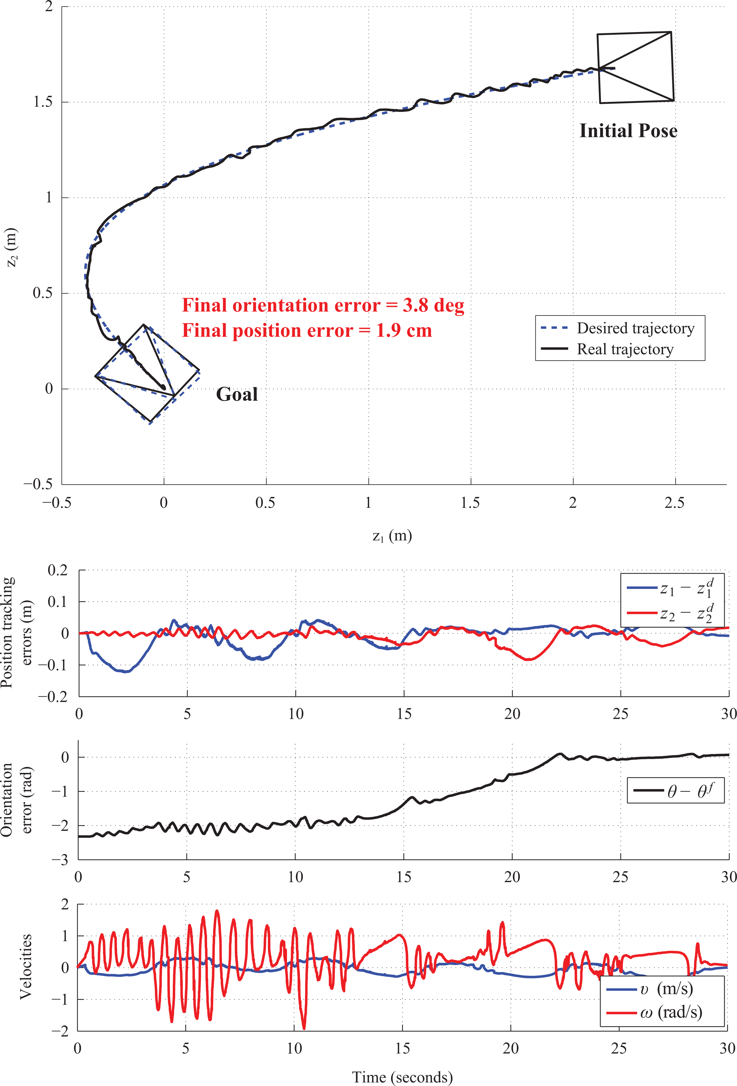
Figure 17 shows the executed and desired trajectories in the experimental runs with external disturbance using the PIC (top) and the STC (bottom). The planned trajectory given by algorithm 1 is a cubic curve. Figures 18 and 19 present the evolution in time of the errors and velocities for the PIC and the STC, respectively. We can see that both controllers maintained the position tracking errors inside the same range of values using similar magnitude of control effort. Moreover, the robot velocities are below of their allowable values ( $v^{max} = 0.7$ m/s and $ω^{max} = π$ rad/s for the TurtleBot 2) in spite of the large transient velocities observed around 6 s due to the external disturbance. In general, we can say that both controllers, PIC and STC, present similar performance for the evaluated conditions. The experimental results of this section are provided as supplementary material in a video. In addition to the results using the PIC and the STC, the video shows a test using only proportional control action, which is not able to achieve an accurate pose-regulation, unless that high gain control will be used, with the risk of exceeding the velocity bounds.

Figure 17.
Executed and desired trajectories for the experiments with a real robot, reaching the origin of the plane in 30 s with desired orientation 315°. Top: Using PIC. Bottom: Using STC. PIC: proportional–integral control; STC: super-twisting control.

Figure 18.
Evolution of the tracking errors and velocities with respect to time using the PIC in the experiments with a real robot. PIC: proportional–integral control.

Figure 19.
Evolution of the tracking errors and velocities with respect to time using the STC in the experiments with a real robot. STC: super-twisting control.

We have carried out a final test in order to present the behavior of the STC for time-varying disturbances (matched bounded disturbances). It can be verified²⁹ that the proof of proposition 3.4 works for general matched bounded disturbances. Thus, the STC is able to deal with bounded time-varying disturbances as shown in Figure 20. In this case, we use $d_{1} = 0.2 (1 + sin (t))$ m/s and $d_{2} = - 0.2 (1 + sin (t))$ rad/s.

Figure 20.
Evaluation of the approach using a real robot for time-varying disturbances with the STC as the controller. STC: super-twisting control.

Discussion of the results and comparison

According to the evaluation of the method, we can say that the proposed approach is a good option for an accurate regulation of the pose of WMRs. It has been compared with existing approaches^11,12 in which the orientation is also included in the control loop and our approach has outperformed them. The main advantage of the method with respect to others is the simplification of the control structure introduced by the fact that the orientation is not directly controlled in the closed-loop. Thus, no explicit planning for the orientation angle is required unlike the classical approach of tracking a virtual reference robot.^5,6,13,14 A benefit of the proposed approach is that it generates continuous and smooth robot velocities using a single controller. This would not be the case if optimal length trajectories (straight lines) will be use. If a desired final pose is required using straight line trajectories, the robot must be controlled in three steps, two different controllers are needed and the switching between them would generate discontinuous robot velocities. Indeed, even the super-twisting sliding mode controller yields continuous control inputs, which mitigates the chattering issue in comparison to classical sliding mode controllers.^9,12 The method allows us to fix a temporal horizon to reach the desired robot pose at difference of classical stabilization/regulation schemes for WMR.^2,5

On the other hand, the trajectory must be correctly selected and accurately tracked in order to achieve good accuracy in the final pose. The generation of the candidate trajectories is really fast and it is done only one time before to start the local navigation. The approach works for any initial and final poses except for those configurations where there is only lateral error between the poses. This is a drawback of the trajectory planning strategy that has some singularities in the computations. However, the singular cases are detectable and the robot can be moved out of that situation before starting the closed-loop control. Finally, the method assumes that the feedback measurements are accurate, which is accomplished in the real experiments and consequently the results are very similar to the simulations. However, the performance might degenerate for instance if estimation of the robot state is carried out from on-board sensors.

Conclusions and future work

In this article, we have addressed the pose-regulation problem of a perturbed underactuated mobile robot, that is, drive the robot to reach simultaneously a desired position and orientation regardless of matched bounded disturbances in the control inputs. The proposed method is a solution for local navigation to move a differential-drive robot between two different poses, focusing on the task to reach the final pose with good accuracy. The pose-regulation problem is faced by tracking adequate trajectories for the position coordinates, such that the robot’s orientation reaches a final desired value due to the nonholonomic motion constraint, since the robot’s heading evolves tangent to the trajectory of position. Two alternatives of robust kinematic controllers are presented to ensure an accurate trajectory tracking, a proportional–integral control and a super-twisting sliding mode control. Moreover, an offline trajectory planning strategy details how to define the adequate trajectories on the basis of quadratic and cubic polynomials and specifies the correct motion direction to track them (forward or backward). We have found that although cubic polynomials provide one more degree of freedom to define the trajectories, they are not always the best option. Quadratic polynomials must be also considered as candidates in order to improve the accuracy in the orientation correction. Compared to classical stabilization/regulation schemes for WMRs, our proposal allow us to define the time of convergence. Moreover, the resulting time-dependent control inputs are smooth. Realistic simulations, comparisons with existing approaches, and experiments in a real setup have shown the good performance of the proposed control scheme.

As future work, we plan to consider the maximum allowable velocities as a constraint in the design of the desired trajectories and to include a collision avoidance strategy while performing robust trajectory tracking. We consider that the algorithm could be extended to deal with obstacles using a waypoints approach given a sequence of desired poses.

Supplementary Material

Supplementary Material

Supplemental material for Simultaneous convergence of position and orientation of wheeled mobile robots using trajectory planning and robust controllers by Héctor M Becerra, J Armando Colunga, and Jose Guadalupe Romero in International Journal of Advanced Robotic Systems

	Proposed PIC	Martins et al.¹²	López-Nicolás and Sagüés¹¹
Orientation (degree)	<1	−4.58	<1	5.16	<1	26.55
Position (cm)	<1	<1	<1	8.37	<1	<1

Footnotes

Acknowledgements

The first two authors of the article were partially supported by CONACYT. The authors would also like to acknowledge the financial support of Intel Corporation for the development of this project.

Declaration of conflicting interests

The author(s) declared no potential conflicts of interest with respect to the research, authorship, and/or publication of this article.

Funding

The author(s) disclosed receipt of the following financial support for the research, authorship, and/or publication of this article: The first two authors of the article were partially supported by CONACYT under grant 220796. The authors would also like to acknowledge the financial support of Intel Corporation for the development of this project.

ORCID iD

Héctor M Becerra

Supplemental material

Supplementary material for this article is available online.

References

Kolmanovsky

McClamroch

. Developments in nonholonomic control problems. IEEE Control Syst 1995; 150(6):20–36.

Oriolo

De Luca

Vendittelli

. WMR control via dynamic feedback linearization: design, implementation, and experimental validation. IEEE Trans Control Syst Technol 2002; 100(6): 835–852.

Skrjanc

Klancar

. A comparison of continuous and discrete tracking-error model-based predictive control for mobile robots. Robot Auton Syst 2017; 870(1): 177–187.

Liu

. Target enclosing and trajectory tracking for a mobile robot with input disturbances. IEEE Control Syst Lett 2017; 10(2): 221–226.

Dixon

Dawson

Zergeroglu

. Robust tracking and regulation control for mobile robots. Int J Robust Nonlinear Control 2000; 100(4): 199–216.

Huang

Zhai

. Disturbance observer-based robust control for trajectory tracking of wheeled mobile robots. Neurocomputing 2016; 1980(2016): 74–79.

Xin

Wang

She

. Robust adaptive tracking control of wheeled mobile robot. Robot Auton Syst 2016; 780(2016): 36–48.

Wang

Miao

Zhong

. Simultaneous stabilization and tracking of nonholonomic mobile robots: a Lyapunov-based approach. IEEE Trans Control Syst Technol 2015; 230(4): 1440–1450.

Dixon

Dawson

DM,

Zergeroglu

. Tracking and regulation control of a mobile robot system with kinematic disturbances: a variable structure-like approach. J Dyn Sys Meas Control 2000 ; 1220(4): 616–623.

10.

Lee

Song

Lee

. Tracking control of unicycle-modeled mobile robots using a saturation feedback controller. IEEE Trans Control Syst Technol 2001; 90(2): 305–318.

11.

López-Nicolás

Sagüés

. Vision-based exponential stabilization of mobile robots. Auton Robot 2011; 30(3): 293–306.

12.

Martins

Elyoussef

Bertol

. Trajectory tracking of a nonholonomic mobile robot with kinematic disturbances: a variable structure control design. IEEE Latin Am Trans 2011; 90(3): 276–283.

13.

Elyoussef

Martins

De Pieri

. PD-super-twisting second order sliding mode tracking control for a nonholonomic wheeled mobile robot. In: 19th IFAC world congress, Cape Town, South Africa, 24–29 August 2014, Elsevier.

14.

Yang

Fan

Xia

. Robust tracking control for wheeled mobile robot based on extended state observer. Adv Robot 2016; 300(1): 68–78.

15.

Donaire

Romero

Perez

. Smooth stabilisation of nonholonomic robots subject to disturbances. In: IEEE international conference on robotics and automation, Seattle, WA, USA, 26–30 May 2015, IEEE.

16.

Hwang

Kang

Hyun

. Robust backstepping control based on Lyapunov redesign for skid steered wheeled mobile robots. Int J Adv Robot Syst 2013; 100(26): 1–8.

17.

Fei

. Velocity tracking control of wheeled mobile robots by iterative learning control. Int J Adv Robot Syst 2016; 130(3): 1–10.

18.

Guerra

Efimov

Zheng

. Finite-time obstacle avoidance for unicycle-like robot subject to additive input disturbances. Auton Robot 2017; 410(1): 19–30.

19.

Canudas de Wit

Khennouf

. Quasi-continuous stabilizing controllers for nonholonomic systems: design and robustness considerations. In: European control conference, Rome, Italy, 5–8 September 1995.

20.

Wang

Low

. Modeling skidding and slipping in wheeled mobile robots: control design perspective. In: IEEE/RSJ international conference on intelligent robots and systems, Beijing, China, 9–15 October 2006, IEEE.

21.

Murray

Sastry

. Nonholonomic motion planning: steering using sinusoids. IEEE Trans Autom Control 1993; 380(5): 700–716.

22.

Pears

. Mobile robot tracking of pre-planned paths. Adv Robot 2001; 150(1): 97–107.

23.

Defoort

Palos

Kokosy

. Experimental motion planning and control for an autonomous nonholonomic mobile robot. In: IEEE international conference on robotics and automation, Roma, Italy, 10–14 April, 2007, IEEE.

24.

Simba

Uchiyama

Sano

. Real-time smooth trajectory generation for nonholonomic mobile robots using Bezier curves. Robot Comput Int Manuf 2016; 41: 31–42.

25.

Zhou

Song

Tian

. Bezier curve based smooth path planning for mobile robot. J Inform Comput Sci 2011; 80(12): 2441–2450.

26.

Choi

Curry

RE,

Hugh Elkaim

. Continuous curvature path generation based on Bezier curves for autonomous vehicles. IAENG Int J Appl Math 2010; 400(2): 91–101.

27.

Ortega

Garcia-Canseco

. Interconnection and damping assignment passivity-based control: a survey. Eur J Control 2004; 10: 432–450.

28.

Khalil

Grizzle

. Nonlinear Systems, third edition, Prentice Hall, Upper Saddle River, New Jersey, USA, 2002.

29.

Moreno

Osorio

. Strict Lyapunov functions for the super-twisting algorithm. IEEE Trans Autom Control 2012; 570(4): 1035–1040.

30.

Michel

. Webots: professional mobile robot simulation. Int J Adv Robot Syst 2004; 10(1): 39–42.

Supplementary Material

Please find the following supplemental material available below.

For Open Access articles published under a Creative Commons License, all supplemental material carries the same license as the article it is associated with.

For non-Open Access articles published, all supplemental material carries a non-exclusive license, and permission requests for re-use of supplemental material or any part of supplemental material shall be sent directly to the copyright owner as specified in the copyright notice associated with the article.

0.00 MB

8.43 MB

	Proposed PIC		Martins et al.¹²		López-Nicolás and Sagüés¹¹
Final errors	Best	Worst	Best	Worst	Best	Worst
Orientation (degree)	<1	−4.58	<1	5.16	<1	26.55
Position (cm)	<1	<1	<1	8.37	<1	<1