Sage Journals: Discover world-class research

Abstract

RGB-D cameras that can provide rich 2D visual and 3D depth information are well suited to the motion estimation of indoor mobile robots. In recent years, several RGB-D visual odometry methods that process data from the sensor in different ways have been proposed. This paper first presents a brief review of recently proposed RGB-D visual odometry methods, and then presents a detailed analysis and comparison of eight state-of-the-art real-time 6DOF motion estimation methods in a variety of challenging scenarios, with a special emphasis on the trade-off between accuracy, robustness and computation speed. An experimental comparison is conducted using publicly available benchmark datasets and author-collected datasets in various scenarios, including long corridors, illumination changing environments and fast motion scenarios. Experimental results present both quantitative and qualitative differences between these methods and provide some guidelines on how to choose the right algorithm for an indoor mobile robot according to the quality of the RGB-D data and environmental characteristics.

Keywords

Motion Estimation Visual Odometry RGB-D Camera Point Cloud Depth Image

1. Introduction

In the last decade, visual odometry (VO) [1] has become very popular in robotics and the computer vision community. VO refers to the problem of recovering camera poses from a set of camera images. Before 2010, most VO methods used stereo cameras or monocular cameras (including perspective and omnidirectional) for motion estimation. From 2010 onwards, consumer-level RGB-D cameras became very popular in the robotics and computer vision community. RGB-D cameras can provide rich 2D and 3D information at the same time, which are well suited to solve the ego-motion estimation problem of an agent. In the past few years, several RGB-D visual odometry [2 –5] estimation methods have been proposed. Existing RGB-D visual odometry methods have shown promising results with high accuracy. However, reliability is still an issue that prevents these methods from on board guidance of a fully autonomous vehicle. These methods may fail in different types of challenging scenarios as they process the sensor data in different ways. Understanding the accuracy changes/reductions of these methods with respect to different challenges is important, and helps us design a more robust motion estimation method for steering an autonomous vehicle.

This paper experimentally compares several real-time RGB-D visual odometry methods including Libviso2 [3], Fovis [4], DVO [5], FastICP [6], Rangeflow [7], 3D-NDT [8], CCNY [9], DEMO [10]. It should be noted that the study of this paper only focuses on visual odometry methods, and therefore various RGB-D V-SLAM algorithms [11], [12] are not considered. Besides, we consider motion estimation methods using data from RGB-D cameras only. Further comparison including inertial-aided methods [13] is not yet considered. The performances of these methods are studied in a variety of challenging scenarios such as in long corridors, illumination changing environments and fast motion scenarios. These scenarios involve low-quality features or featureless moments, which the existing method may or may not be able to handle. Experimental comparison of the aforementioned methods shows that the performance of each odometry estimation method depends on the quality of RGB-D data as well as environmental characteristics. Though some of these methods can obtain very good estimation in certain environments, none of them can perform very well in all environments. The experiment results provide some guidelines on how to use different visual odometry methods according to the quality of RGB-D data and environment characteristics.

The rest of this paper is organized as follows. In section II, we discuss the related work. Section III describes the selected representative odometry estimation methods. We validate the performance of each method by using real datasets in section IV and we conclude in section V.

2. Related work

Visual odometry is the process of estimating the ego-motion of an agent (e.g., vehicle and robot) using only the input of a single or multiple cameras attached to it. The term VO was coined in 2004 by Nister in his landmark paper [1]. VO is a particular case of structure from motion (SFM) in the computer vision community [14]. SFM is more general and tackles the problem of 3D reconstruction of both the structure of the environment and camera poses from a set of camera images. The final structure and camera poses are usually refined with an offline optimization process, whose computation time grows with the number of images. On the contrary, VO only focuses on estimating the 3D pose of the camera in real time. It is also worth mentioning another very popular topic in the robotics community: visual simultaneous localization and mapping (V-SLAM) [15], [16]. The goal of V-SLAM is to obtain a global, consistent estimate of the robot path. It keeps a track of a map of the environment. When the robot returns to a previously visited area, a loop closure will be detected that is used to reduce drift in both the map and camera path. Compared to V-SLAM, VO tries to recover the camera path incrementally, pose after pose. In some VO methods, local optimization methods (e.g., windowed bundle adjustment) may potentially be used to reduce the drift. In essence, VO only cares about the local consistency of the trajectory and map, while V-SLAM is concerned with global map consistency.

VO can be used as a front-end block for the V-SLAM algorithm. For a complete V-SLAM algorithm, some backend blocks such as loop-closure detection and graph optimization are still needed. Generally, V-SLAM is potentially much more precise, but is also more complex and computationally expensive. In recent years, RGB-D SLAM has also become very popular in the robotics community [17], [12]. The main difference between RGB-D SLAM and traditional V-SLAM is that RGB-D SLAM systems use both RGB and depth images from a RGB-D camera. In this paper, we mainly want to compare some motion estimation methods than can be potentially used on a small micro aerial vehicle (MAV). However, nowadays most V-SLAM and RGB-D SLAM algorithms cannot run in real time on computation-limited embedded computers. Therefore, in this paper we focus on real-time odometry methods that can be potentially used on a MAV.

Currently, visual odometry methods mainly use three kinds of cameras for motion estimation, namely stereo cameras, monocular cameras and RGB-D cameras. Stereo VO methods try to recover the camera trajectory using consecutive images from two cameras, while monocular VO methods try to recover the camera motion through only one (perspective or omnidirectional) camera. The advantage of stereo VO is that it can get absolute depth information through the triangulation algorithm by using the calibrated baseline. The disadvantage is that stereo VO will become monocular VO when the distance to the observed scene is much further than the length of the baseline of the stereo camera. For monocular VO methods, a shortcoming is that there is an unknown absolute scale problem in the estimation. For more details of traditional VO methods, the interested readers are referred to visual odometry tutorials [2]. From 2010 onwards RGB-D cameras became very popular since they can simultaneously provide RGB and depth images at a high frame rate, which also do not suffer from the unknown scale problem of monocular VO if the depth information is available. Since then, several RGB-D visual odometry estimation methods have been proposed by using visual data and/or depth data. These methods can be roughly divided into three categories according to what kind of data are mainly used, namely image-based methods, depth-based methods and hybrid-based methods. It should be noted that this is just a kind of rough classification. In fact, all of the methods use depth information. The difference is that for the image-based methods, they almost still follow the traditional stereo VO or monocular VO pipeline (which compute the depth values from triangulation), but use the depth information from depth images; for the depth-based methods, they only use depth information from depth images for motion estimation without using any RGB information; for the hybrid-based methods, they do not exactly follow the pipeline of traditional VO methods, but try to use both RGB and depth information in different ways to improve the robustness and accuracy of motion estimation.

The first category is image-based methods which usually depend on a lot of information from RGB images. Three different kinds of algorithms are widely used. The first kind is a sparse visual feature-based method [4, 18]. These methods usually extract sparse visual features first and then find the feature correspondences by matching the descriptors of each feature. After this they usually use RANSAC-based methods to reject the outliers. Then, the 3D information of each feature is calculated through triangulation. Finally, the transformation matrix is calculated by minimizing the re-projection errors. The second kind is still a sparse feature-based method but uses depth information directly from depth images [4] [18]. These methods also detect and extract visual features using different kinds of feature detectors (such as SIFT, FAST, SURF), and then finding the feature correspondences. However, they do not triangulate the features to get depth information, but instead use the depth information from the RGB-D's depth image directly. Finally, the transformation matrix is also calculated through minimization of the re-projection error. The third kind is called a dense feature-based method [5],[19] which is quite different from sparse visual feature-based methods because it uses the whole image to estimate the transformation. This method assumes a world point p observed by two cameras which is assumed to yield the same brightness in both images. The goal is to find the camera motion that best satisfies the photo-consistency constraint over all pixels.

The second category is depth-based methods which usually depends on information from depth images. There are also several different kinds of methods. The first kind is the 3D feature-based method [20, 21], which can be seen as an extension of the 2D cases. In these methods, 3D features like point, line or plane features will be detected and extracted. Then, the feature correspondences will be found using different kinds of matching methods. After this, the transformation matrix can be calculated by minimizing the distance error function of the feature correspondences. These methods are usually widely used in the registration of 3D laser point clouds. However, it is worth noting that the point clouds from 3D laser scanners usually have less noise than RGB-D cameras and the long measurement range also helps them to find more 3D features in a single scan. Unfortunately, commodity-level RGB-D cameras have a very limited measurement range and their data are also very noisy compared to laser scanners. Therefore, usually 3D feature registration methods do not work very well for RGB-D cameras. Besides, most of them cannot run in real time. The second kind is Normal Distribution Transform (NDT) based method [22],[23]. These methods consider a point cloud as a distribution. They use the Normal Distribution Transform to map a point cloud to a smooth surface representation, described as a set of local probability density functions, each of which describes the shape of a section of the surface. They can then find the relative transformation between two point clouds by finding the optimal point-to-distribution or distribution-to-distribution matching. NDT is a very good solution for 3D point cloud registration; however, it is sensitive to segmentation because large spatial cells filter out relevant details, whereas small cells augment the computational cost. Besides, it is also sensitive to initial guess and not very fast. The third kind uses the point cloud directly[6], [24]. These methods firstly convert the depth image into 3D point cloud and then use ICP-based methods, which are widely used in 3D registration areas, to estimate motion. The advantage of these methods is that they can get very accurate estimation results using a dense point cloud. The disadvantage is that these methods are time consuming. However, in recent years researchers have begun to propose fast ICP-based registration methods. The fourth kind is based on depth image and range flow theory[25], [7]. The key idea of these methods is similar to dense visual odometry using RGB images. These methods use the range flow constraint to calculate the transformation between two consecutive frames. It assumes that a 3D point X (measured in the depth camera's coordinate system) is captured at pixel position x = (x,y)^T in depth map Z_t. This point undergoes a 3D motion ΔX which results, first, in an image motion Δx between frames, and second in a change in the depth ΔZ of the 3D point captured at this new image location x +Δx. By using this constraint, these methods can calculate the relative transform between two consecutive frames. The advantage of these methods is that all calculations are directly based on the depth image without detecting any 3D features or doing any additional transform, and is therefore much faster.

The third category is hybrid-based methods [9, 26 –30]. They can also be divided into several kinds. The first kind is switch strategy-based methods. The key idea is that they improve RGB-D VO performance by switching from one method to another. For example, Leishman et al. [27] proposes a switching strategy which can switch to 2D laser odometry, 3D visual odometry and 2D visual odometry automatically according to the quality of RGB and depth images. Whelan et al. [28] integrate fovis and dense visual odometry with ICP for dense RGB-D mapping on a powerful CPU and GPU. The second kind is the two-stage method. The key idea of these methods is that they usually use RGB information to get an initial guess of the transformation and then use a dense point cloud or local optimization algorithm to refine the transformation. For example, the Adaptive Iterative Closest Keypoint algorithm exploits both point position and visual appearance information [26]. It calculates the initial registration based on appearance and refines the final registration using 3D points. Dryanovski [29] proposes a two-stage incremental registration algorithm for RGB-D images. In the first stage, edge features are detected from colour and depth images, and these edge points are then fed into ICP to calculate the initial motion estimation. In the second stage, the initial guess is refined by applying the GICP algorithm on the frame-to-frame dense point cloud. Herry [30] also proposes a two-stage RGB-D ICP using sparse features and ICP. Andreasson [8] proposes the use of 2D image features and NDT to obtain a more robust and faster estimation. The key idea is to detect 2D visual features and find corresponding regions from previous frame to current frame and then use RANSAC to find a consistent alignment. After that, the geometrical information around the selected features is utilized as an input to a fast 3D-NDT distribution-to-distribution method to refine the transformation. Zhang [10] proposes a depth enhanced RGB-D visual odometry method. The difference of this method to other RGB-D visual odometry methods is that it considers both feature with and without depth information. Most RGB-D visual odometry methods discard the image features that do not have a depth value. However, this paper thinks even those features without depth are still useful for motion estimation. By doing so, this method can get better results if the depth information is not sufficient. This method also uses local bundle adjustment to refine the pose estimation. The third kind is the joint optimization method. The key idea is to combine different error functions (e.g., 2D re-projection error and 3D Euclidean distance error) into one error function and minimize the combined error function to obtain a final estimation. For example, Herry [30] proposes a joint optimization method that combines sparse feature reprojection error and point-to-plane distance error into one error function to estimate the final motion. Whelan et al. [28] combine the dense intensity error and point-to-point distance error to obtain a more robust odometry estimation for 3D mapping. Besides the above ideas, Dryanovski [9] proposes a Kalman filtering-based fast visual odometry method. They first compute the locations of sparse features in the RGB image and their corresponding 3D coordinates in the camera frame. They then align the 3D features against a global 3D features map expressed in the fixed coordinate frame using a modified ICP method. At the same time, they estimate the uncertainty in the depth readings and use a Kalman filter to update the global 3D feature map.

3. Examined Odometry Estimation Methods

As described in Section II, existing visual odometry methods can be roughly divided into three categories according to what kind of sensor data are used. Here, we select eight representative real-time odometry estimation methods and compare them by using the real datasets. Note that there are also some excellent methods [31],[21],[28] that can estimate the camera motion accurately, but we have not selected them because they are either too slow or they depend on a powerful GPU. The selected methods are shown in Table 1. In the following, the selected methods are briefly described.

Table 1.

Selected RGB-D visual Odometry Methods

Category	Method	Data type	Features	Aligned Frames
	Libviso2		2D Visual Features	Frame-to-Frame
Image-based	Fovis	RGB+Depth	2D Visual Features & Depth	Frame-to-Keyframe
	DVO		2D Image Intensity & Depth	Frame-to-Frame

Depth-based	FastICP Rangeflow	Point Cloud Depth Image	3D Point Cloud Depth	Frame-to-Local Map Frame-to-Frame

	Realtime NDT		2D Visual Features & Cloud	Frame-to-Frame
Hybrid-based	CCNY	RGB+Depth	3D Visual Features Cloud	Frame-to-Local Map
	DEMO		2D visual Features & Depth	Frame-to-Frame with BA

3.1 Image-based Methods

Many odometry estimation methods proposed in the past several years are based on visual information. Here, we select three representative methods since they use the image information in different ways. RGB-D cameras like the Kinect are monocular vision systems. If one wants to use them to estimate the motion by using image data only, it is necessary to know external information to solve the unknown scale problem. In fact, the selected methods here all use depth information. However, since they depend on much information from RGB images, we call them image-based methods.

3.1.1 Libviso2

Libviso2 [3] is a fast algorithm for computing the 6 DOF motion of a moving mono/stereo camera. For the stereo version of libviso2, the key idea is to extract robust sparse features, find the feature correspondences, get the depth information through triangulation and finally minimize the re-projection error of sparse feature matches to obtain the transformation. Let π^(l)(X;r, t) denote the projection matrix that projects a 3D point X to a pixel x_i^(l) on the left image plane, and let π^(r)(X;r, t) be the projection onto the right image plane. Libviso2 uses Gauss-Newton optimization algorithm to minimize

\sum_{i = 1}^{N} {‖ x_{i}^{(l)} - π^{(l)} (X_{i}; r, t) ‖}^{2} + {‖ x_{i}^{(r)} - π^{(r)} (X_{i}; r, t) ‖}^{2}

(1)

The monocular version assumes that the camera is moving at a known and fixed height over ground and uses this constraint to estimate the unknown scale. In order to use libviso2 with RGB-D cameras, we actually change the RGB-D camera into a virtual stereo camera using the depth information. We create a virtual camera using the depth information of each pixel with a fixed baseline. If the RGB pixels do not have depth information, we discard them. We then feed both RGB images of the real camera and virtual camera into libviso2 to calculate the odometry.

3.1.2 Fovis

Fovis [4] is a visual odometry method that estimates the 3D motion of a camera using a source of depth information for each pixel. It first detects FAST features in each image. Then, the depth corresponding to each feature is extracted from the depth image. Features that do not have an associated depth are discarded. After that, each feature is assigned an 80–byte descriptor. Features are then matched across frames by comparing their feature descriptor values using a mutual-consistency check. Then, the inliers are detected by computing a graph of consistent feature matches and using a greedy algorithm to approximate the maximal clique in the graph. Finally, the motion estimate is computed from the matched features in three steps. First, it uses Horn's absolute orientation method to provide an initial estimate by minimizing the Euclidean distance between the inlier feature matches. Then, the motion estimate is refined by minimizing feature re-projection error using a nonlinear least-squares solver. Finally, feature matches exceeding a fixed threshold are discarded from the inlier set and the motion estimate is refined once again. Fovis uses a keyframe technique to reduce short-scale drift.

3.1.3 DVO

In contrast to sparse feature-based methods, dense visual odometry [5] methods want to fully exploit both the intensity and the depth information provided by RGB-D sensors. Dense visual odometry uses all colour information of the two consecutive images and the depth information of the first image. This approach is based on the photo-consistency assumption, which means a world point p observed by two cameras is assumed to yield the same brightness in both images.

I_{1} (X) = I_{2} (τ (ξ, X))

(2)

where τ(ξ,X) is the warping function that maps a pixel coordinate X ∈ ℜ² from the first image to a coordinate in the second image given the camera motion ξ ∈ ℜ⁶. The goal is to find the camera motion ξ that minimizes the photo-metric error over all pixels. In order to improve the robustness of estimation, DVO applies a probabilistic framework to estimate the transform, where they use a robust sensor model based on the t-distribution, and a motion prior based on a constant velocity model. DVO also uses a coarse-to-fine strategy to make the estimation more robust against large motion. It constructs an image pyramid and computes a first estimate on a coarse image scale and iteratively refines this estimate on finer scales.

3.2 Depth-based Methods

There are also many people working on motion estimation using only depth data. Actually, this is widely studied in computer graphics where it is necessary to register different views of scans to reconstruct an object or environment. Many excellent registration algorithms have been proposed in the past decades, such as the 3D point-based method [32], plane-based method [21] and 3D Normal Distribution Transform [22]. Most of these registration algorithms are very accurate, but are usually slow and computationally expensive. Here, we select two methods that are very fast to run in real time. One is the FastICP method which mainly uses the point cloud for motion estimation. The other one is Rangeflow, which only uses depth image for motion estimation.

3.2.1 FastICP

The Iterative Closet Points (ICP) algorithm was proposed by Besl and McKay in 1992 [33] to solve the 3D rigid shape registration problem. The classical pairwise rigid registration problem can be described as: given a set of source points X = {x_i,i = 1, …, n} and Y = {y_i,i = 1, …, n}, we want to find the optimal transformation by minimizing the energy function as:

\arg \min R, t, Y \sum_{i = 1}^{N_{p}} φ (R x_{i} + t, y_{i})

(3)

where R is a rotation matrix, t is a translation vector, φ is the error metric function.

The key concept of the standard ICP algorithm can be summarized in two steps: 1) the alignment is fixed, a set of closest corresponding points Y is computed. 2) the 3D point correspondences are fixed, compute a transformation which minimizes distance between corresponding points. Iteratively repeating these two steps typically results in convergence to the desired transformation. According to [34], the following six steps influence the performance of ICP:

Select a subset of points in one or both point clouds.

Match these points to samples in the other point cloud.

Weigh the corresponding pairs appropriately.

Reject certain pairs by some strategies.

Assign an error metric.

Minimize the error metric.

In this paper, ethzasl-icp-mapping [6] developed by Pomerleau is chosen for comparison because it mainly focuses on robotic applications. This fast ICP follows the standard ICP pipeline as described in [34].

3.2.2 Rangeflow

This method uses the so-called range flow constraint to calculate the frame-to-frame motion estimation [7], [25], [35]. It assumes a 3D point X (measured in the depth camera's coordinate system) is captured at pixel position x = (x,y)^T in depth map Z_t. This point undergoes a 3D motion ΔX which results, first, in an image motion Δx between frames, and second in a change of the depth ΔZ of the 3D point captured at this new image location x + Δx. Thus, the range flow constraint is formulated as

Z_{τ} (x + Δ x) = Z_{t} (x) + Δ Z

(4)

In this paper, our implementation of the range flow odometry estimation method is based on [35]. This method utilizes a weighted least-squares minimization of the difference between the measured rate of change of depth at a point and the rate predicted by the so-called range flow constrain equation. It assumes that most of the surface is smooth enough that local tangent planes can be constructed and that the motion between frames is smaller than the size of most features in the range image. This method does not depend on detecting and matching of high-level features in the range images.

3.3 Hybrid-based Methods

Odometry estimation methods based on both image and depth information have become very popular in recent years. The most commonly used idea is first using 2D image features to obtain an initial guess and then using point registration methods (such as ICP, NDT) to refine the estimation. There are also some people who try to combine image-based error metrics and depth-based error metrics into one integrated error metric, then optimize the integrated error function to find the optimal transform [28], However, these methods depend on a powerful computer for complex optimization. Here, we choose three real-time RGB-D visual odometry methods for comparison.

3.3.1 Realtime NDT

Andreasson [8] proposes a real-time local visual feature boosted NDT method for RGB-D odometry estimation. The key idea is to detect 2D visual features and find corresponding regions from the previous frame to current frame and then use RANSAC to find a consistent alignment. After that, the geometrical information around the selected features is efficiently utilized as an input to a fast 3D-NDT-D2D method [22] to refine the transformation. Instead of computing the 3D-NDT representation of the full depth images, this method only considers the immediate local neighbourhoods of each of the detected local visual features points. By doing so, the number of Gaussian components can be substantially decreased. Thus, the whole estimation process can be calculated in real time.

3.3.2 CCNY

Dryanovski [9] from the City College of New York (CCNY) proposes a fast visual odometry method based on visual features and depth information. The key idea of ccny_rgbd visual odometry is to align 3D features against a global 3D feature map. They first compute the locations of sparse features in the RGB image and their corresponding 3D coordinates in the camera frame. Then, they align the 3D features against a global 3D features map expressed in the fixed coordinate frame using a modified ICP method. After calculating the transformation, the global 3D feature map is updated using a Kalman filter. Any features from the incoming image that cannot be associated are considered to be new features in the global 3D feature map. To guarantee constant time performance, they bound the number of 3D feature in the global 3D feature map. Once the map size is bigger than a threshold, the oldest features are dropped. Since this method does not need 2D feature descriptor computation and feature correspondence matching, it saves a lot of computation. Besides, by performing alignment against a global 3D feature map instead of only the last frame, this method can significantly reduce the drift of the pose estimation.

3.3.3 DEMO

Zhang [10] proposes a depth enhanced monocular odometry (DEMO) method. The difference of this method to other RGB-D visual odometry methods is that it considers both features with and without depth information. Most RGB-D visual odometry methods drop the image features that do not have a depth value. However, this paper thinks even those features without depth are still useful for motion estimation. In this method, first, visual features are tracked using the KLT method. Depth images are then registered using the estimated motion. Visual features are associated with a depth value using the registered point cloud. If a visual feature does not have corresponding depth value from the point cloud but has been tracked for longer than a certain distance, then its depth value will be calculated through triangulation using the first and the last image frames. By doing so, they have three different kinds of visual features; one is visual feature with depth from depth image, the other one is visual features with depth from triangulation and the third is feature with no depth information. They use these three kinds of features to calculate the frame-to-frame relative transformation. After this, they use a local bundle adjustment (BA) method to refine the estimation. Finally, they combine the high frequency frame-to-frame motion estimation with the low frequency refined motion estimation and generates the integrated motion transform as the final odometry estimation.

4. Experiments and analysis

In this part, we first compare the accuracy of each method by using the TUM RGB-D dataset¹ which has accurate ground truth for evaluation [36]. Then, in order to evaluate robustness, we also record some datasets in very challenging environments, such as long clear corridors, structured and cluttered environments, dramatic illumination changing environment, etc. Then, we validate the performance of each algorithm on an Asus UX31E Ultrabook (Quad-core 1.7GHz CPU and 4GB Memory) running ROS fuerte and PCL1.7. The RGB-D sensor is Asus Xtion Pro Live which records the RGB-D image at 15Hz with 640×480 resolution.

It should be noted that all the methods evaluated in this paper are sensitive to the choice of parameters, which might influence the final accuracy and timing results. From our experience, for a certain dataset better results may be achieved for a method if its parameters are carefully tuned according to that specific dataset. However, this same set of parameters may work undesirably for another dataset. Here, we only select the RGB-D fr2/desk dataset for tuning all the parameters of each method. The reason that we choose this dataset is that this dataset has relative rich visual and geometric features which are good for all the examined methods. Besides, this dataset is also the easiest dataset of all the datasets used in this paper. We carefully tune all the parameters for each method based on the RGB-D fr2/desk dataset. Some important parameters are listed in Table 2. However, since we want to get a general comparison of these methods, we do not tune the parameters again for the rest of the test datasets. The parameters of each method are kept the same in all tests.

Table 2.

Some Important Parameters For Experiments

Method	Parameters	Values	Description
Libviso2	param_nms_n	4	Minimum distance between maxima in pixels for non-maxima-suppression
	param_match_binsize	50	Interest point peakiness threshold
	param_match_radius	50	Matching width/height, which affects efficiency
	paramnms_tau	200	Matching radius (du/dv in pixels)
Fovis	max_pyramid_level	3	Maximum pyramid levels for detecting visual features
	max_keypoints_per_bucket	25	The number of features in each bucket with the strongest FAST corner score are remained
	min_features_for_estimate	10	The minimum number of features for odometry estimation
	feature_searchwindow	25	The window size for matching features
DVO	coarest_level	3	The coarsest level of image pyramid for motion estimation
	MaxIterationsPerLevel	50	Max Iterations in each Pyramid level
	UseWeighting	true	Whether the weighting function is used
	weight_method	t-distribution	T-distribution weight function is used for optimization
FastICP	MaxDistDataPointsFilter	7	Threshold for filtering out points beyond maximum range
	TrimmedDistOutlierFilter	0.75	This filter considers as inliers a certain percentage of the links with the smallest norms
	minOverlap	0.4	The minimum threshold overlap ratio between current frame and previous frame for motion estimation
Rangeflow	downsample	6	Uniform downsampling step size
	gaussian_mask_size	9	Mask size for Gaussian smoothing
	rows and cols	60, 80	The final downsampled depth image size for motion estimation
Realtime NDT	support_size	15	Neighbourhood size of one pixel for searching correspondence
	image_scale	0.25	Image size downsampling scale
	detector_thresh	200	The threshold value for detecting SURF features
	subsample_step	5	Point cloud downsampling scale
CCNY	detector_type	GFT	Type of feature detector
	max_iterations	10	The max iterations for ICP registration
	max_model_size	10000	The max local 3D map size kept for alignment
	n_nearestneighbors	4	Number of nearest neighbors found from model
	maxcorrespdisteucl	0.15	Threshold of Euclidean distance between feature correspondences
DEMO	maxFeatureNumPerSubregion	15	Max number of features kept in each sub region
	winSize	21	Window size for feature tracking
	timeDis	5	Keep the last five seconds point cloud as local map
	cloudSkipNum	5	Uniform downsampling step size of point cloud
	cloudSkipNum	5	Uniform downsampling step size of point cloud

4.1 Accuracy Comparison using Benchmark Dataset

In this section, we use TUM RGB-D datasets to test the estimation accuracy of each method. The dataset contains the colour and depth images along with the ground-truth trajectory. The data are recorded at full frame rate (30 Hz) and sensor resolution (640×480). The ground-truth trajectory is obtained from a high-accuracy motion-capture system with eight high-speed tracking cameras (100 Hz). Here, we choose two datasets to evaluate the accuracy of each method. The experimental results are shown in Table 3.

Table 3.

Mean and standard deviation of translational and rotational errors of each method

Methods	fr2/desk				fr1/room
Methods	x̄(m)	σ	θ(deg)	σ	x̄(m)	σ	θ (deg)	σ
Libviso	0.036	0.031	1.516	0.735	0.063	0.051	2.431	1.432
Fovis	0.012	0.007	0.526	0.307	0.056	0.035	2.377	1.328
DVO	0.024	0.012	0.982	0.512	0.058	0.045	2.396	1.539
FastICP	0.022	0.022	0.942	0.618	0.066	0.103	3.012	2.704
Rangeflow	0.031	0.021	1.556	0.972	0.092	0.074	5.389	4.563
Realtime NDT	0.024	0.015	1.228	0.735	0.065	0.032	2.851	1.412
CCNY	0.020	0.012	0.762	0.457	0.057	0.036	2.790	1.797
DEMO	0.023	0.015	0.997	0.628	0.075	0.044	2.881	1.506

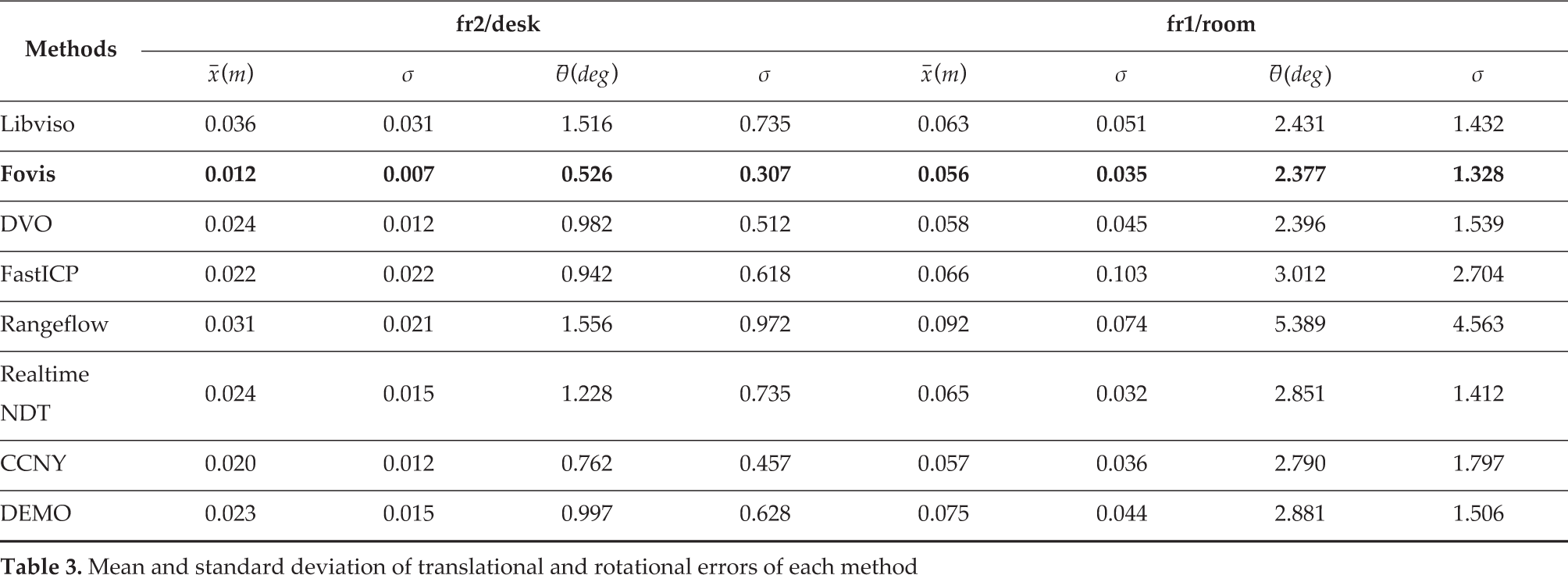
We use the relative pose error and absolute pose trajectory error metric [36] to measure the drift and global consistency of the visual odometry system, respectively. We calculate the ratio of pixels in the image that contain a valid depth compared to the total number of pixels in the image to estimate the quality of the point cloud. We compute the average and standard deviation of the grey-scale-pixel values of the RGB image as a measurement of the amount of light available in the image, which is a simple way to estimate the quality of an image.

The first dataset is freiburg2/desk. For this sequence, the RGB-D data are recorded in a typical office scene with two desks, a computer monitor, chairs, etc. The Kinect is moved around two tables so that the loop is closed. The average translational and angular velocity are 0.193m/s and 6.338 deg/s respectively. The mean intensity changes from 73.1 to 153.8, and the standard deviation changes from 76.1 to 42.1. However, the depth coverage changes from 85.3% to 53.9%. Therefore, the RGB information is good while the depth information is not very good. The mean and median relative pose error of each method is shown in Table 3 and the absolute pose trajectory error of each method is shown in Fig. 1. From the results, we can see that Fovis gets the best accuracy. Besides, the image and depth combined methods also obtain very good and similar results. The reason that visual information-based methods are good is that they can accurately and robustly detect and match feature correspondences since the RGB information is very good and the motion is relatively slow in this dataset.

Figure 1.

Absolute Pose Trajectory Error

The second dataset is freiburg1 room. In this dataset, the sequence is filmed along a trajectory through a typical office. It starts with the four desks but continues around the wall of the room until the loop is closed. The depth coverage changes from 83.8% to 54.9%. The mean intensity changes from 169.5 to 77.8 and standard deviation changes from 101.6 to 41.8. The experiment results are also shown in Table 3. In this dataset, there are some fast rotations. The average translational velocity is 0.334 m/s and the average angular velocity is 29.882 deg/s, which is much faster than the freiburg2/desk dataset. Therefore, it is a little bit difficult for sparse feature-based methods. The advantage of the visual feature-based method is not that obvious in this dataset, as you can see the mean translation and rotation error of depth-based methods are similar to visual information-based methods. In this dataset, the Rangeflow method gets the worst performance. The potential reason for this is that the fast motion of the camera breaks the small motion assumption of this method. The sampling rate is not fast enough to ensure a small relative motion between two consecutive frames. Generally for DVO and Rangeflow, a fast sampling rate is good for odometry estimation.

4.2 Robustness Validation in Challenging Environments

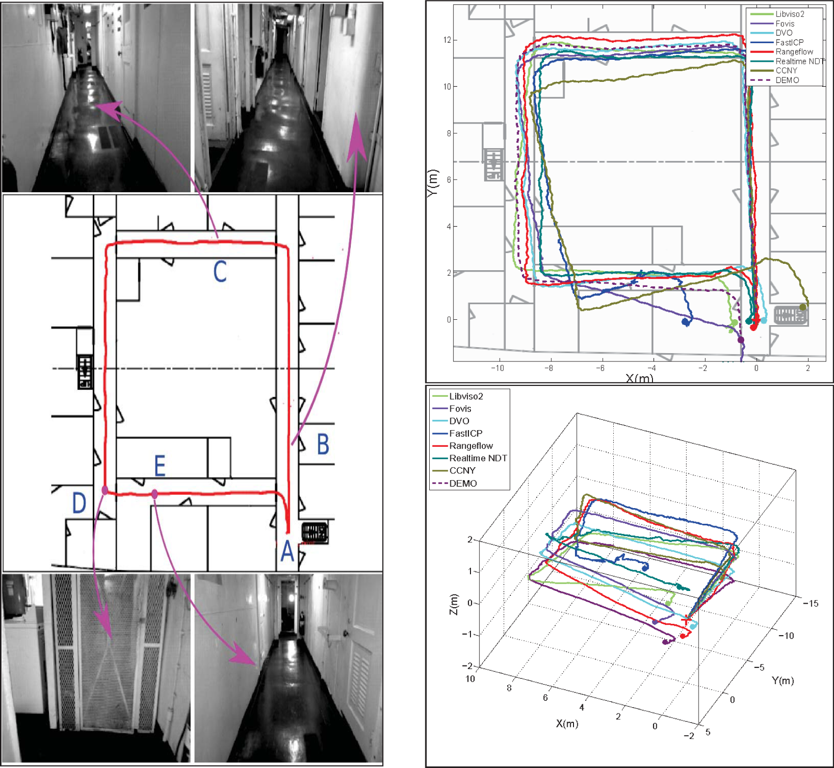
In this part, we collect some datasets in different kinds of environments to test the robustness of each method. Though it is quite easy to get ground truth in outdoors (highly accurate GPS) and small indoor environments (Motion Capture System, such as Vicon), it is very difficult to obtain accurate 6DOF ground truth in large indoor environments. Since it is very hard to obtain ground truth in large indoor environments, the camera is started and stopped at the same position. Therefore, we can use loop-closing error to evaluate the estimation performance of each method to some extent. We define the loop-closing error as the gap between the two ends of a trajectory output compared to the total length of the trajectory. The loop-closing errors of each method are shown in Table 4. Note that in Fig. 2 –Fig. 5, the trajectory is projected onto the x − y plane. Therefore, if the x, y errors in the figure are very small but the loop-closing error is very big, this means there is a big drift in z coordinates. In order to show the clear differences between each method, an experimental video can be found at https://www.dropbox.com/s/561itmojn1cka1c/IJARS.mp4?dl=0.

Table 4.

Loop-closing error

Methods	Loop-closing error
Methods	Test1	Test2	Test3	Test4
Libviso	3.77%	1.45%	failed	13.6%
Fovis	7.41%	1.12%	failed	7.79%
DVO	2.00%	7.26%	16.86%	6.72%
FastICP	6.91%	4.58%	7.03%	3.16%
Rangeflow	2.57%	4.27%	3.89%	10.44%
Realtime NDT	5.83%	5.74%	failed	5.13%
CCNY	6.88%	3.24%	18.46%	2.46%
DEMO	3.15%	9.12%	failed	2.99%

Figure 2.

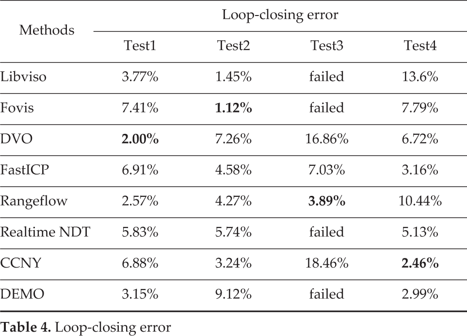
Test 1: Long Corridor Environment. The left part shows the approximate traversing trajectory when recording the dataset and some snapshots of the environment along the trajectory. We start from point A, then go along the corridors in counter-clockwise direction to place B, C D, E and finally go back to the start point again. The top right figure shows the projected trajectories of each odometry method on the map. The bottom right figure shows the 3D trajectory of each method. At place C and E, FastICP fails due to insufficient constraints in the moving direction. At place D, fovis fails due to repetitive features on the wall.

Figure 3.

Test 2: Complex Environment. The left part shows the approximate traversing trajectory when recording the dataset and some snapshots of the environment along the trajectory. We start from place A, then go through doors to get to place B, C and D, then finally go back to start point A. The top right figure shows the projected trajectories of each odometry method on the map. The bottom right figure shows the 3D trajectory of each method. In this dataset, place A is a little bit cluttered and place B is close to the wall. Place C is long corridor and place D is a spacious area. Those areas pose different challenges for each odometry method.

Figure 4.

Test3: Illumination changing Environment. The left part shows the approximate traversing trajectory when recording the dataset and some snapshots of the environment along the trajectory. We start from place A where the illumination is very good, then enter into a dark conference room to place B, and move counter-clockwise to place C and D, and finally go back to place A. The top right figure shows the projected trajectories of each odometry method on the map. The bottom right figure shows the 3D trajectory of each method. As you can see that when we enter into or exit the room, the illumination changes a lot. Most methods do not work well after arriving at place B except Rangeflow, FastICP and DVO. At place B, FastICP and Rangeflow both suffer from the degeneration problem as you can see a sudden orientation change occurred.

Figure 5.

Test3: Fast motion scenario. The top part shows the projected trajectories of each odometry method on the floor map and some snapshots of the environment along the trajectory. The bottom figure shows the 3D trajectory of each method.

Test 1: long corridor environment. Very clear long corridors usually pose big challenges for visual odometry methods. In this experiment, the mean intensity of images changes from 164.5 to 59.4 and the depth coverage ratio changes from 90.9% to 79.3%. It seems that both RGB and depth information are very good. However, in this long corridor, the floors and walls are very smooth. There are many places where only small objects on the wall or door frames can be used to estimate the translation. Therefore, this environment is very challenging for both visual and depth-based method since there are only few visual features and geometry features. Fig. 2 shows the experimental results of different methods. As you can see, in this environment DVO has the best result, while Fovis fails before the robot enters into the last corridor section. It should be noted that Fovis does not output any estimation when the algorithm finds there are not enough feature correspondences. A very short failure in Fovis will only increase the drift of the odometry, which will not cause the whole estimation to totally fail. The FastICP method also has a similar failure detection technique. When the overlapping of two consecutive point clouds is too small or not enough point correspondences are available, FastICP will not output any results. Fovis's failure is due to many repetitive textures around the corner of the last corridor section, as shown in the top right picture in Fig. 2, where Fovis fails to detect and track features when the camera turns quickly around that corner. However, Libviso2 can still track the features successfully around that corner. It seems Libviso2's feature tracking method is more robust than Fovis. The reason why DVO can succeed is that it depends on the whole image information other than sparse visual features which are difficult to detect in this environment. Sometimes, though some sparse visual features can be detected, they may be discarded due to a lack of corresponding depth value. This is why the DEMO method is also better than other sparse visual feature-based methods. The FastICP method also fails to estimate the translation in the last corridor section. The reason for failure is that there are not enough constraints in the last corridor for the ICP method to estimate the translation.

Test 2: structured and cluttered environment: The second experiment is in a more complex environment. In this environment, sometimes there are very long corridors, sometimes there are cluttered rooms and sometimes there are very spacious rooms. We use this environment to check whether all the methods can adapt to the changes of environmental structure. The mean intensity of images changes from 173 to 47 and the depth coverage ratio changes from 88.7% to 47.0%. As you can see, the quality of both image and depth changes much more than the first experiment. Fig. 3 shows the experiment results. From the experiment results, you can see that Fovis has the smallest loop-closing error and Libviso2 also gets very good estimation. The pure depth-based methods, FastICP and Rangeflow, get similar loop-closing error, but both have a big drift. DVO works well on most occasions except around some turning points, where most algorithms become poor. The reason is that the passage is very narrow (less than 1 metre) and the quick turn happened at a place very close to a wall, where Xtion RGB-D cameras cannot attain good RGB and depth data since the fast motion and the minimum measurement range of Xtion is 80cm. Therefore, it is very difficult for most of the evaluated methods to estimate the transform accurately.

Test 3: Illumination changing environment. The third experiment is a conference room where there is a big desk and many chairs. In this experiment, dramatic illumination changes occur when the robot enters into and goes out of the conference room. The mean intensity changes from 169.2 to 3.5. The conference room is very dark where the intensity is just about 3.5~30, which is very challenging for visual-based methods. Fortunately, we can still get a good point cloud in this environment, where the depth coverage ratio changes from 71.5% to 90.1%. The experiment result is shown in Fig. 4. There is no doubt that depth-based methods will be better than visual-based methods in this environment. In our experiment, we found that Rangeflow achieves the best performance. To our surprise, dense visual odometry can still work almost all the time except in very dark areas (the mean intensity is less than 10). It seems that DVO is much more robust than sparse feature-based methods in this test. However, even depth-based methods achieve better results in this test, and they also encounter the degeneration problem. As you can see around place B in 4, both FastICP and Rangeflow slide far away from the true position.

Test 4: Fast motion scenario. This dataset is recorded in a typical office environment where there are many tables, desks and computers. Therefore, this environment has lots of very good geometric and textural features for motion estimation. When recording the data, we keep rotating the camera with a relatively fast speed. The experimental result is shown in Fig. 5. As you can see from the RGB images, there is an obvious motion blur. The loop-closing error of each method is also shown in Table 4. From the results, we can see that for relative fast motion, FastICP is better than the image-based method. The reason for this is that fast motion can cause motion blur (Asus Xtion RGB-D camera is a rolling shutter camera) which is very bad for feature detecting and matching while the point cloud is not too bad. This is why the RGB and depth combined methods can also get better results. In this test, the CCNY method gets the smallest loop-closing error. One reason for this is that it uses robust 2D visual feature detectors and 3D feature matching methods. Another reason why FastICP and CCNY are better than other methods is that both of them use frame to local map matching strategy. When there was a large motion, frame-to-frame or frame-to-keyframe based methods could not find good feature correspondences. However, since a local map is much bigger than one image frame, there are many more features or points to match, which makes it much better for fast motion. The NDT method is also better than image-based methods. That benefits from NDT using a two-stage optimization strategy. Though the fast motion decreases the estimation accuracy of the first stage, most of the time the second stage can refine the estimation of the first stage by using NDT registration on dense point clouds. However, if the motion is too fast, the first stage might be unable to achieve a good motion estimation. This means the initial guess of the second stage is not very good, and therefore the final estimation is sometimes still not very good.

4.3 Speed and CPU Usage Comparison

Besides the accuracy and robustness, the computational performance of each method is also very important, especially for the application on computation resources limited robot platform. We test the speed and CPU usage of each method using an Asus UX31E Ultrabook (Quad-core 1.7GHz CPU, 4GB Memory). Both RGB and depth images are of 640×480 size. The experimental results are shown in Table 5. In our experiment, all the tested methods can run in real time on our laptop. Most of them can run at more than 20Hz. It should be noted that Libviso2 and DEMO are multi-thread programs, while others are single-thread programs. In libviso2, one node is for feature matching and another node is for odometry estimation. While there are three nodes in DEMO, one is for feature tracking, another one is for depth processing and the third one is for odometry estimation. Out of all of the methods, Rangeflow has the best speed and the lowest CPU usage, which is also much faster than image-based methods. The reason why Rangeflow is so fast is that it only needs to compute the gradients of a down-sampled depth image without any feature detection and matching, which saves a lot of computation time. Besides, it is only a frame-to-frame estimation method, which does not use any image pyramid, keyframe, local-map or local BA techniques to improve robustness.

Table 5.

Computational performance on the Test2 Dataset

Method	Algorithm Runtime(ms)				Avg CPU
	Mean	Min	Max	StdDev	Usage
	Libviso2	39.5	18.9	180.2	18.9	29.8%
Fovis	20.3	10.8	47.9	4.5	13.5%
DVO	52.4	20.1	242.8	11.2	22.6%
FastICP	50.3	13.3	350.0	34.0	26.1%
Rangeflow	6.33	1.50	36.5	4.0	12.5%
Realtime NDT	29.9	11.5	133.6	11.8	21.9%
CCNY	28.2	12.3	101.9	13.4	26.3%
DEMO	21.9	10.8	80.3	6.5	24.5%

4.4 Analysis and Discussion

From the experiment results, it is clear that though some of the examined methods can achieve good results in specific environments, none of them can perform very well in all kinds of environments: they all have their own advantages and disadvantages.

Visual information-based methods are usually more robust and accurate than point cloud-based methods. However, they have the following disadvantages. First, the environments must have enough illumination. Second, the environments must have good texture features to be detected. Third, most of them discard the feature points that do not have depth information. Therefore, for spacious environments where depth information is not sufficient, most of them also cannot attain good estimation.

For depth information-based methods, the advantage is that they can be used in very dark environments. However, they also have some shortcomings. First, the effective measurement range of the RGB-D camera is very limited. Therefore, there are often not enough points with constraints in spacious areas like atria and long hallways, which often cause the degeneration problem. Second, the depth data of the consumer-level depth camera is very noisy. However, we still need to downsample it to reduce computation time. Therefore, the estimation accuracy of the point cloud-based method is not as accurate as visual information-based methods in most cases.

Methods that use both image and depth information usually they take advantage of both information types. Most times these methods work very well. However, most of them depend on good RGB images, and if they cannot find very good visual features most of them will obtain bad estimation results even if the depth is still very good. Therefore, the issue of how to use depth and image information more effectively and efficiently is still a problem.

By analysing the characteristics of each method and the RGB-D data, we can get some basic ideas on how to use the RGB-D camera for robust and accurate odometry estimation. If the RGB and depth information are both available and good, we think that we should use both kinds of information as much as possible for robustness consideration. If the RGB image has abundant features but very limited depth information, we should still consider how to use those features that do not have depth information. If the depth image has abundant geometric features but the RGB information is bad, we can depend on depth information-based methods. If both RGB and depth information are unavailable, we can only use other sensor information for short time prediction; for, example fusing visual odometry with IMU.

In addition, through analysing each method from theoretical and experimental aspects, we can also attain some important tips for using each method. Libviso2 was originally designed for stereo cameras, which follows a traditional stereo visual odometry pipeline. Its performance mainly depends on robust and accurate sparse visual feature detection and matching. It needs enough and accurate sparse feature correspondence to do triangulation and estimation. Another problem is that even when there are enough features, when the camera performs pure rotation the linear system to calculate the fundamental matrix degenerates. Therefore, when using libviso2 one should avoid motion that has pure rotation without translation. Though the estimation pipeline of Fovis is similar to libviso2, it has several techniques to make it more accurate and efficient than libviso2. Firstly, it uses an image pyramid to enable more robust feature detection at different scales. Secondly, it uses the keyframe technique to reduce short-scale drift. A shortcoming of Fovis is that it doesn't work well in environments with many repetitive features. DVO tries to use all of the dense visual information without detecting any sparse features; therefore, theoretically it can be more robust and accurate than sparse feature-based methods. However, in order to achieve this the relative motion between two consecutive image frames must be small enough. Even though DVO uses the image pyramid technique to make it more robust against large motion, it is still not good for large motion. Therefore, a higher sampling rate is better for DVO. This is almost the same for range flow-based methods, which are also direct motion estimation methods based on depth images instead of RGB images. In this paper, the rangeflow method is only a frame-to-frame estimation method, and is therefore fast but not accurate or robust. It does not use either image pyramids or keyframe techniques to improve robustness. The FastICP method constructs local maps to reduce the drift; however, the ICP-based method is still not very fast. A big problem for depth-based methods is that they both easily suffer from degeneration problems, which are very common in indoor environments. To achieve a good performance of rangeflow and FastICP, one should avoid making the camera only see a wall, especially during rotation, otherwise both of them will output the estimated results sliding away from the true position. For the realtime NDT method, it really depends on a good initial guess from sparse visual features. For the refine stage, a good segmentation is also very important. The CCNY method estimates the motion using 3D features, providing four kinds of feature detectors including ‘GFT’, ‘SURF’, ‘STAR’ and ‘ORB’. Most of the time we found that ‘GFT’ is the best choice for robustness and efficiency. Besides, the maximum iteration and model size of ICP registration really influences the speed and accurate of the estimation. The DEMO method is a little different from others since it tries to reconstruct features without depth values, while other methods directly discard those features. There are two important things that will influence the performance of DEMO: First, the maximum features number and searching window size for feature tracking, and secondly the local point cloud size and density. The performance of the DEMO method is almost the same as other sparse feature-based methods in rich visual feature environments with depth values, but it will outperform other methods in depth insufficient environments.

5. Conclusions

In this paper, a detailed analysis and comparison of several visual odometry methods using RGB-D cameras has been presented. Representative approaches were compared on real data from publicly available datasets and author-collected datasets in several challenging environments. As the experimental results show, the performance of each odometry estimation method depends on the quality of RGB-D data and the environment characteristics. The experiment results provide some guidelines on how to use different visual odometry methods.

If the environment has rich visual features and illumination is also good, we should generally consider image-based or hybrid-based methods since they are more robust than depth-based methods. However, for featureless or dark environments, depth-based methods are the best choices. More specifically, in environments with abundant texture features, if the image grey value is also good, Fovis is the best choice for accuracy and speed. If the illumination is relatively dark, DVO is the best choice since it works much better than sparse feature-based methods in bad illumination environments. If the illumination is very bad (Mean grey value is smaller than 10) or in featureless environments, then Rangeflow is the best choice since it is much faster than ICP-based methods. If there is no sufficient depth information, DEMO is better than other methods. For fast-motion scenarios, generally local map-based methods are better than others. The choice of the best algorithm depends on the quality of RGB-D data and the characteristics of the practical environment.

Footnotes

6. Acknowledgements

Research presented in this paper was funded by China Scholarship Council, NSFC under grant no.61040014, No. 61005085 and Fundamental Research Funds for the Central Universities under grant no.N120408002 and 2012QNA4024. The authors would also like to thank Sebastian Scherer for his valuable discussions and help.

1

(accessed December 15, 2013)

References

Nister

Naroditsky

, and Bergen

Visual odometry. Proc. 2004 IEEE Comput. Soc. Conf. Comput. Vis. Pattern Recognition, 2004. CVPR 2004., 1, 2004.

Scaramuzza

Davide

Fraundorfer

Friedrich

, and By Scaramuzza

Davide

. Visual Odometry [Tutorial]. IEEE Robotics & Automation Magazine, 18(4):80–92, December 2011.

Geiger

Andreas

Ziegler

Julius

, and Christoph

Stiller

. StereoScan: Dense 3D reconstruction in realtime. In 2011 IEEE Intelligent Vehicles Symposium (IV), pages 963–968. Ieee, June 2011.

Huang

and Abraham

Bachrach

. Visual odometry and mapping for autonomous flight using an RGB-D camera. Int. Symposium on Robotics Research, pages 1–16, 2011.

Kerl

Christian

Sturm

Jurgen

, and Daniel

Cremers

. Robust odometry estimation for RGB-D cameras. In 2013 IEEE International Conference on Robotics and Automation, pages 3748–3754. IEEE, May 2013.

Pomerleau

François

Colas

Francis

Siegwart

Roland

, and Magnenat

Stéphane

. Comparing ICP variants on real-world data sets. Autonomous Robots, 34(3):133–148, February 2013.

Graeme

Jones

. Accurate and Computationally-inexpensive Recovery of Ego-Motion using Optical Flow and Range Flow with Extended Temporal Support. In Procedings of the British Machine Vision Conference 2013, pages 75.1–75.11. British Machine Vision Association, 2013.

Henrik

Andreasson

and Todor

Stoyanov

. Real time registration of RGB-D data using local visual features and 3D-NDT registration. Proc. of International Conference on Robotics and Automation (ICRA) Workshop on Semantic Perception, Mapping and Exploration (SPME), 2012.

Ivan

Dryanovski

and Valenti

Roberto G.

Fast visual odometry and mapping from RGB-D data. In 2013 IEEE International Conference on Robotics and Automation, pages 2305–2310. IEEE, May 2013.

10.

Zhang

Kaess

Michael

, and Sanjiv

Singh

. Realtime Depth Enhanced Monocular Odometry. 2014IEEE/RSJ International Conference on Intelligent Robots and Systems, September 2014.

11.

Klose

Sebastian

Heise

Philipp

, and Alois

Knoll

. Efficient compositional approaches for real-time robust direct visual odometry from RGB-D data. 2013IEEE/RSJ International Conference on Intelligent Robots and Systems, pages 1100–1106, November 2013.

12.

Kerl

Christian

Sturm

Jurgen

, and Daniel

Cremers

. Dense visual SLAM for RGB-D cameras. 2013IEEE/RSJ International Conference on Intelligent Robots and Systems, pages 2100–2106, November 2013.

13.

Guo

Chao X.

and Roumeliotis

Stergios I.

IMU-RGBD camera navigation using point and plane features. 2013 IEEE/RSJ International Conference on IntelligentRobots and Systems, pages 3164–3171, November 2013.

14.

Longuet-Higgins

H. C.

A computer algorithm for reconstructing a scene from two projections. Nature, 293(5828):133–135, September 1981.

15.

Davison

A.J.

Real-time simultaneous localisation and mapping with a single camera. In Proc. Ninth IEEE Int. Conf. Comput. Vis., pages 1403–1410 vol.2. IEEE, 2003.

16.

Georg

Klein

and David

Murray

. Parallel Tracking and Mapping for Small AR Workspaces. In 2007 6th IEEE ACM Int. Symp. Mix. Augment. Real., pages 1–10. IEEE, November 2007.

17.

Gibson

Huang

Shoudong

Zhao

Liang

Alempijevic

Alen

, and Gamini

Dissanayake

. A robust RGB-D SLAM algorithm. In 2012 IEEE/RSJ Int. Conf. Intell. Robot. Syst., pages 1714–1719. IEEE, October 2012.

18.

Quijada

and Eduardo

Zalama

. Fast 6D Odometry Based on Visual Features and Depth. The 12th International Conference on Intelligent Autonomous Systems, 193(June):245–256, 2013.

19.

Tykkala

Tommi

Audras

Cedric

, and Comport

Andrew I.

Direct Iterative Closest Point for real-time visual odometry. In 2011 IEEE International Conference on Computer Vision Workshops (ICCV Workshops), pages 2050–2056. IEEE, November 2011.

20.

Xiao

Junhao

Adler

Bejamin

, and Houxiang

Zhang

. 3D point cloud registration based on planar surfaces. In IEEE International Conference on Multisensor Fusion and Integration for Intelligent Systems, pages 40–45, 2012.

21.

Pathak

Kaustubh

Birk

Andreas

Ius

Narunas

VasìŇ

KevicìŇ

, and Jann

Poppinga

. Fast Registration Based on Noisy Planes With Unknown Correspondences for 3–D Mapping. IEEE Transactions on Robotics, 26(3):424–441, June 2010.

22.

Stoyanov

Magnusson

Andreasson

, and Lilienthal

A. J.

Fast and accurate scan registration through minimization of the distance between compact 3D NDT representations. The International Journal of Robotics Research, 31(12):1377–1393, September 2012.

23.

Magnusson

Martin

Lilienthal

Achim

Duckett

Tom

, and Uk

Lincoln L N

. Scan registration for autonomous mining vehicles using 3D-NDT. Journal of Field Robotics, 24(10):803–827, October 2007.

24.

Segal

Aleksandr V

Haehnel

Dirk

, and Sebastian

Thrun

. Generalized-ICP. Robotics: Science and Systems, 2009.

25.

Horn

Berthold K.P.

and Harris

John G.

Rigid body motion from range image sequences. CVGIP Image Underst., 53(1):1–13, January 1991.

26.

Ekekrantz

Johan

Pronobis

Andrzej

Folkesson

John

, and Patric

Jensfelt

. Adaptive iterative closest keypoint. In 2013 European Conference on Mobile Robots, pages 80–87. IEEE, September 2013.

27.

Leishman

Robert C.

Koch

Daniel P

McLain

Timothy W.

, and Randal

Beard. Robust Motion Estimation using an RGB-D Camera. In AIAA Infotech@ Aerospace Conference, pages 1–13, 2013.

28.

Whelan

Thomas

Johannsson

Hordur

Kaess

Michael

Leonard

John J

, and John

McDonald

. Robust real-time visual odometry for dense RGB-D mapping. In 2013 IEEE International Conference on Robotics and Automation, pages 5724–5731. IEEE, May 2013.

29.

Dryanovski

Ivan

Jaramillo

Carlos

, and Jizhong

Xiao

. Incremental registration of RGB-D images. In 2012 IEEE International Conference on Robotics and Automation, pages 1685–1690. IEEE, May 2012.

30.

Henry

Peter

Krainin

Michael

Herbst

Evan

Ren

Xiaofeng

, and Dieter

Fox

. RGB-D mapping: Using Kinect-style depth cameras for dense 3D modeling of indoor environments. The International Journal of Robotics Research, 31(5):647–663, February 2012.

31.

Trevor

Alexander J. B.

and Henrik

Christensen. RGB-D edge detection and edge-based registration. In 2013 IEEE/RSJ International Conference on Intelligent Robots and Systems, pages 1568–1575. IEEE, November 2013.

32.

Rusu

R.B.

Blodow

Marton

Z.C.

, and Beetz

Aligning point cloud views using persistent feature histograms. In 2008 IEEE/RSJ International Conference on Intelligent Robots and Systems, pages 3384–3391. IEEE, September 2008.

33.

Besl

P.J.

and McKay

H.D.

A method for registration of 3-D shapes. IEEE Transactions on Pattern Analysis and Machine Intelligence, 14(2):239–256, 1992.

34.

Rusinkiewicz

and Marc

Levoy

. Efficient variants of the ICP algorithm. In Proceedings Third International Conference on 3–D Digital Imaging and Modeling, pages 145–152. IEEE Comput. Soc, 2001.

35.

Tarifa

Mariano Jaimez

. Difodometry: Fast visual odometry for range cameras. http://www.mrpt.org/list-of-mrpt-apps/application-difodometry-camera/, Accessed: June 2014.

36.

Sturm

Wolfram

Burgard

, and Daniel

Cremers

. Evaluating Egomotion and Structure-from-Motion Approaches Using the TUM RGB-D Benchmark. IEEE/RJS International Conference on Intelligent Robot, 2012.

Experimental Evaluation of RGB-D Visual Odometry Methods

Abstract

Keywords

1. Introduction

2. Related work

3. Examined Odometry Estimation Methods

3.1 Image-based Methods

3.1.1 Libviso2

3.1.2 Fovis

3.1.3 DVO

3.2 Depth-based Methods

3.2.1 FastICP

3.2.2 Rangeflow

3.3 Hybrid-based Methods

3.3.1 Realtime NDT

3.3.2 CCNY

3.3.3 DEMO

4. Experiments and analysis

4.1 Accuracy Comparison using Benchmark Dataset

4.2 Robustness Validation in Challenging Environments

4.3 Speed and CPU Usage Comparison

4.4 Analysis and Discussion

5. Conclusions

Footnotes

6. Acknowledgements

1

References