
Abstract
A stable walking motion requires effective gait balancing and robust posture correction algorithms. However, to develop and implement such intelligent motion algorithms remains a challenging task for researchers. Effective sensory feedback for stable posture control is essential for bipedal locomotion. In order to minimize the modelling errors and disturbances, this paper presents an effective sensory system and an alternative approach in generating a stable Centre-of-Mass (CoM) trajectory by using an observer-based augmented model predictive control technique with sensory feedback. The proposed approach is used to apply an Augmented Model Predictive Control (AMPC) algorithm with an on-line time shift and to look ahead to process future data to optimize a control signal by minimizing the cost function so that the system is able to track the desired Zero Moment Point (ZMP) as closely as possible, and at the same time to limit the motion jerk. The robot's feet are fitted with force sensors to measure the contact force's location. An observer is also implemented into the system.
1. Introduction
The development of bipedal humanoid robots began more than 30 years ago. Despite numerous research efforts, controlling a bipedal robot is still an extremely challenging task in terms of adaptability, robustness and stability. The most common approaches are the Linear Inverted Pendulum Model (LIPM) and the Zero Moment Point (ZMP) method as in [1,2]. The problem with the LIPM method is that it is a non-minimum phase system [3], which produces a undershoot response to a step input. In order to compensate for this undesired effect, a new observer-based Augmented Model Predictive Control (AMPC) method is proposed in this paper. Together with the sensory feedback system, this method reduces the jerk produced by the ground landing impact forces and is also able to improve the overall system performance of ZMP tracking under external disturbances. The effectiveness of the proposed scheme is demonstrated in a simulation and in comparison with the preview control method. Section two explains the robot unique mechanical structure. The robot is designed with a lightweight material and can be correctly modelled like a ‘point-mass' system. Section three presents how the sensory system is deployed to enhance the effectiveness of the feedback system. Section four provides an overview of the robot's electronics control architecture and the various balance control subsystems. Section five gives a detailed implementation of the proposed AMPC control approach. Section six concludes our proposed methods and recommends future work.
2. Robot Mechanical Structure
The TPinokio robot is approximately 1.5m tall and weighs approximately 45kg. It has more than twenty-five degrees of freedom (DoF) as depicted in Figure 1. It is constructed from lightweight aluminium material, as such, the joint-link inertia is negligible. All the components are housed in a compact-joint housing mechanism. It has a simple kinematic structure and it can be modelled as a simplified ‘point-mass' system, as in [4]. The robot's feet are fitted with force sensors to measure the ZMP location. The measured ZMP value is used to determine the system tracking error and to provide a feedback signal to an observer [5] in order to improve the system stability.

TPinokio design and stick-diagram)
2.1 Modular Joint Design
In order to accurately model the robot as a point-mass system, all the joints are designed with lightweight aluminium and assembled in a compact housing, as depicted in Figure 2 and Figure 3.

Modular parts
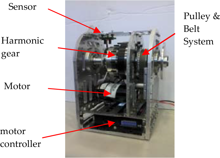
Compact modular design of the joint
3. Robot Sensory System
In order to improve the stability and enhance the robot walking posture, an intelligent sensory system is deployed at strategic joint positions to provide sensory feedback.
3.1 Foot force sensor
Each foot sole and toe are fitted with four load-cell sensors, a total of eight load-cell sensors per foot, as depicted in Figure 4.
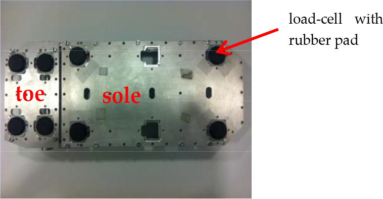
Load-cell sensors and its mounting location.
The value of the sensor's reading is fed through a filter/amplifier to remove noises. The data is then sent to the controller for processing.
During the single support and double support phases, the ZMP can be calculated as depicted in Figure 5a and 5b and Equation (2.1) and (2.2), respectively.


Force/ZMP coordinates in single foot support
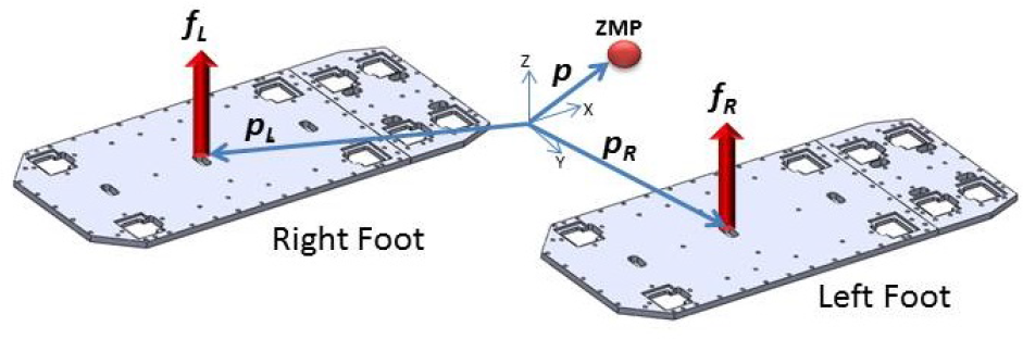
Force/ZMP coordinates in double support phase
3.2 Inertia and vision sensor
The robot guidance and navigation system includes a nine-axis gyro sensor that provides orientation and angular motion feedback to the stabilizer controller. The path search and obstacle avoidance controller receives feedback from the 270° laser scanner and the USB CAM. As depicted in Figure 6 (a), (b) and (c).

(a) 9-axis gyro sensor, (b) Laser scanner, (c) USB CAM
3.3 Position sensor
Each individual joint of the robot is fitted with an absolute encoder and an optical sensor, as depicted in Figure 7. The optical sensor is for initialization; the absolute encoder is used for real time tracking of the joint's position.

Absolute position sensor in all joints.
3.4 Absolute ground sensor
Two tri-axis tilt sensors are fitted at the robot ankle joint to measure the ankle's pitch and the roll angles, as depicted in Figure 8. The function of these sensors is to sense the x-y tilt angles of the feet and ground contact point. This is to provide feedback from the ground conditions to the robot stability controller, so that the controller can adjust the posture of the robot accordingly and to react to any external forces to keep the robot in a stable condition to prevent it falling.

Tilt sensor at ankle joint
4. Robot Control Architecture
4.1 Control electronics
The main communication bus for the robot control electronics and sensory system is the CANbus. The secondary buses are the USB and RS232, as depicted in Figure 9.
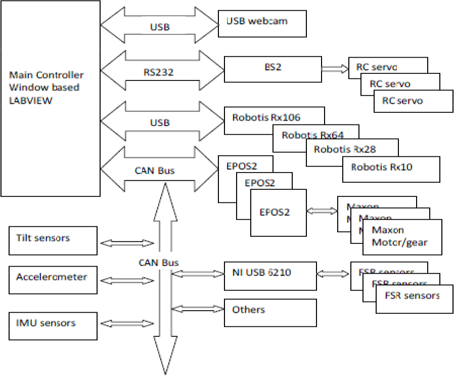
Control electronics and sensory system architecture
4.2 Balancing Control with sensors feedback
During the walk cycle, the hip/pelvis link of the robot may not always maintain in a horizontal position as depicted in Figure 10. This is due to gravitational vibration and other structural mechanism problems. As a result, the swing leg is prone to collide with the stance leg. A nine-axis IMU Figure 6(a), is mounted on to the pelvis position to measure the robot's roll/pitch/yaw motion and two three-axis tilt sensors are mounted on the robot ankle joint to measure the floor inclination during walking and when the swing foot initially touches down on the ground surface. The sensor's reading will compensate for the ground condition error accordingly, as shown in Figure 10 and Figure 11. [6].

Frontal roll angle compensation of swing leg
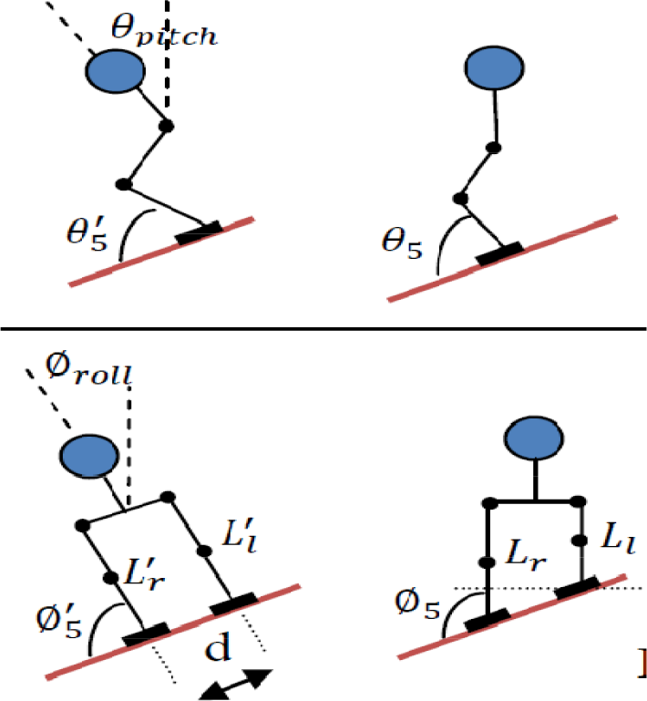
Sensor feedback compensation on non-planar surface For the sagittal plane, where k is the gain:
Collision avoidance control:
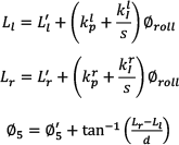
The compensation angle for right hip roll, where kr is the gain:
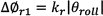

The compensation angle for left hip roll, where kl is the gain:

Slope balancing control:
The slope compensator for the sagittal plane and frontal plane are as depicted in Figure 11.

For the frontal plane, where kp and kr are the gain:
5. Robot Modelling
5.1 Kinematics model
The forward kinematics of the robot is defined by applying the Denavit-Hartenberg (D-H) convention method [7], as depicted in Figure 12.


TPinokio forward kinematics D-H model
The inverse kinematics of the robot can be solved by searching for the value of the joint q by applying the Newton-Raphson iteration algorithm method [7].

where q is the joint angular position and J is the Jacobian matrix.
Inverse kinematics iteration technique [7].
Set the initial counter = 0.
Find or guess an initial estimate q(0).
Calculate the residue δT(q(i)) = J(q(i))δq(i).
If ever element T(q(i)) of or its norm ‖T(q(i))‖ is less than a tolerance, ‖τ(q(i))‖ < ε then terminate the iteration. The q(i) is the desired solution.
Set i = i + 1 and return to step 3.
This concludes the kinematics modelling.
5.2 Dynamics model
Bipedal humanoid robots are locomotion systems with rigid bodies; the required torque command to cause each joint variables q(t) to follow a desired path motion as a function of time can be derived by using the Lagrange equations of motion [8]. The three models at different stages of the walking phases are derived from the general form:

The matrix M is the inertia matrix, C denotes the Coriolis matrix, G is the gravity vector, B is the mapping matrix of the joint torque to the generalized forces and U is the applied torques.
Under-actuated phase
The under-actuated phase occurs when the heel of the stance leg rises from the ground and the robot begins to roll over the toe. Because there is no actuation between the toe and the contact surface, the dynamics of the robot in this phase is equivalent to an n-DoF robot with un-actuated feet. The dynamics are:

Where qu = [q1, q2 … qn] are the joint angles and Uu = [u1, u2 … qn–1] is the vector of torque applied at the joint. Bu is the mapping matrix.
Fully actuated phase
The fully actuated phase is defined as when the stance foot lands flat on the contact surface without slipping and the stance leg ankle acts like an actuated pivot. The dynamics of the robot during the fully actuated phase are equivalent to an n-1 DoF robot without the stance foot and with actuation at the stance ankle [8]. The fully actuated phase dynamics equation is:

Where qa = [q1, q2 … qn–1] is the ankle configuration, un–1 is the input at the ankle joint and Ub = [u1, u2 … un–2] is the vector of inputs applied at the other joints. Ba1 and Ba2 are the mapping matrices.
Double-support (impact) phase
The double-support phase involves the instantaneous impact and reaction forces at the leg ends. It is modelled as the total resultant forces and torques acting on the swing foot at the ankle joint. The dynamics model is:

Where Fext denotes the external forces acting on the robot due to the contact between the swing/landing foot and the surface.
By applying an inverse kinematics algorithm, the joint angle q for the desired geometric path of the three reference points (Left-foot ΣL, right-foot ΣR and Pelvis ΣH) of the bipedal robot can be derived, as depicted in Figure 13. The joint actuator torque command can then be calculated by substituting the desired joint angle q into Equation (5.4), (5.5) and (5.6).

Robot geometry and coordinate
5.3 Momentum and motion trajectory
The transformation from the foot-toe/CoM trajectories into an individual link joint trajectory can be carried out with the momentum calculation method [9]. The four reference frames of the robot are as shown in Figure 13 and are defined as ΣW ΣH ΣL ΣR], which denote the world frame, the pelvis frame, the left-foot frame and the right-foot frame, respectively. The position and orientation of a point in space can be are represented by a translational vector p(3×1) and an orientation matrix R(3×3) as shown:

The foot velocity of the two legs can be written as:

where JlegL and JlegR are a (6×6) Jacobian matrix of the robot's leg with rHL = pL – pH and rHR = pR – pH. *̂ is an operator, which translates the vector (3×1) rHL and rHR into a (3×3) skew symmetric matrix r̂HL and r̂HR. The linear momentum P(3×1) and the angular momentum ℒ(3×1) of the CoM of the robot can be calculated by the following formula:

where m is the robot's total mass, I˜3×3 is the inertia matrix with respect to the CoM. r̂HC is the skew symmetric matrix of rHC. M and H are the inertial matrices of the joints. For a stable and fast walking motion, the angular momentum of the CoM is set to zero (i.e., no rotation) and the translation movement of the CoM can be calculated from Equation (5.9). By definition P = mCȯMx and setting ℒ=0 yields:
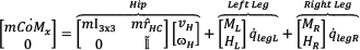
For a given leg velocity ([vL, ωL] T , [vR, ωR] T ), the Hip velocity can be obtained by:

Finally, the leg's joints angle can be calculated by:

This concludes the robot dynamics modelling.
5.4 Joint trajectory generation
The robot's joint trajectory is generated using seven degrees of polynomial; this is to ensure that the all the joint s's start and stop at the same time and its position, velocity, acceleration and jerk parameters are all zero when it reaches the desired angular position. For example, to move the angular position of a joint with a zero jerk start-stop path for q(0) = 10° and q(f) = 45° in T=1s, the unknown coefficient q0, a1, a2, … a7 can be found by solving the following set of polynomial equations:

Set the eight boundary conditions to:

Solving the coefficients (a0 to a7) with the following matrix:

The path motion is as shown in Figure 14.
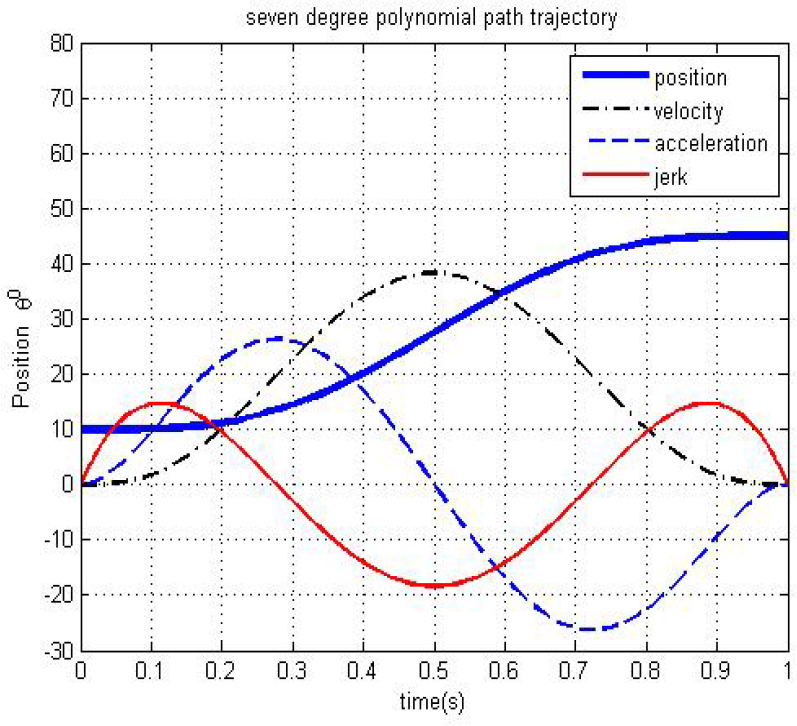
Angular position trajectory of the joint
5.5 Foot trajectory
The basic parameters for a humanoid walking are steplength S, pelvis height Z, foot lifting height H and frontal-shift F, as depicted in Figure 15.

A typical bipedal walking gait.
For TPinokio, a parabolic trajectory for the foot motion of the swing leg is shown in Figure 16.

Foot path trajectory.

Where S is the stride, H is the maximum foot height T is the one step period and the stride frequency is
5.5 Inverted Pendulum Model
In order to define the relationship of the ZMP and the CoM trajectories, a simplified Linear Inverted Pendulum Model (LIPM) is studied in this paper. During walking, in the leg swing phase, the CoM of the robot may be modelled as a ‘point mass' [5] and it is assumed to be connected to the stance foot like an inverted pendulum on a moving base, as depicted in Fig. 17.

Linear Invert Pendulum Model (LIPM).
The Linear Inverted Pendulum Model (LIPM) equations under constraint control (moving along a defined plane) are given as [3]:

The above equations are decoupled, and they can be expressed independently. As such, for the subsequence equations, only the sagittal plan (x-axis) is presented. The frontal plane (y-axis) can be derived with the same procedures. With an extra variable, the system jerk, u is defined as:

The LIPM can be expressed in state-space model.
Continuous time state-space form:
The ZMP equation for the sagittal plane can be expressed in a continuous time state-space model as:

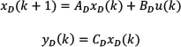
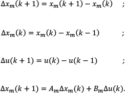
Discrete time state-space form:
Equation (5.18) is discretized with intervals of constant length T, yielding:

Equations (5.18) and (5.19) can be used to determine the dynamic behaviour of the LIPM system.
5.6 Characteristics of a Linear Inverted Pendulum Model
The LIPM is a non-minimum phase system; there is an undesired zero at the RHP, as shown in Figure 18 and Figure 19, for the continuous time system and the discrete time system, respectively (with zcom = 0.5m, g = 9.81). The undesired zero appears outside the unit circle. The RHP zero will produce a reverse action undershoot transient response [3] to a step input. Care should be taken to address this initial ‘water-bed’ effect, as this may cause the bipedal robot to lose balance and fall.
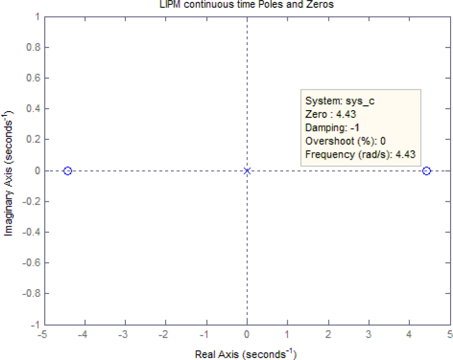
Continuous time poles and zeros plot.
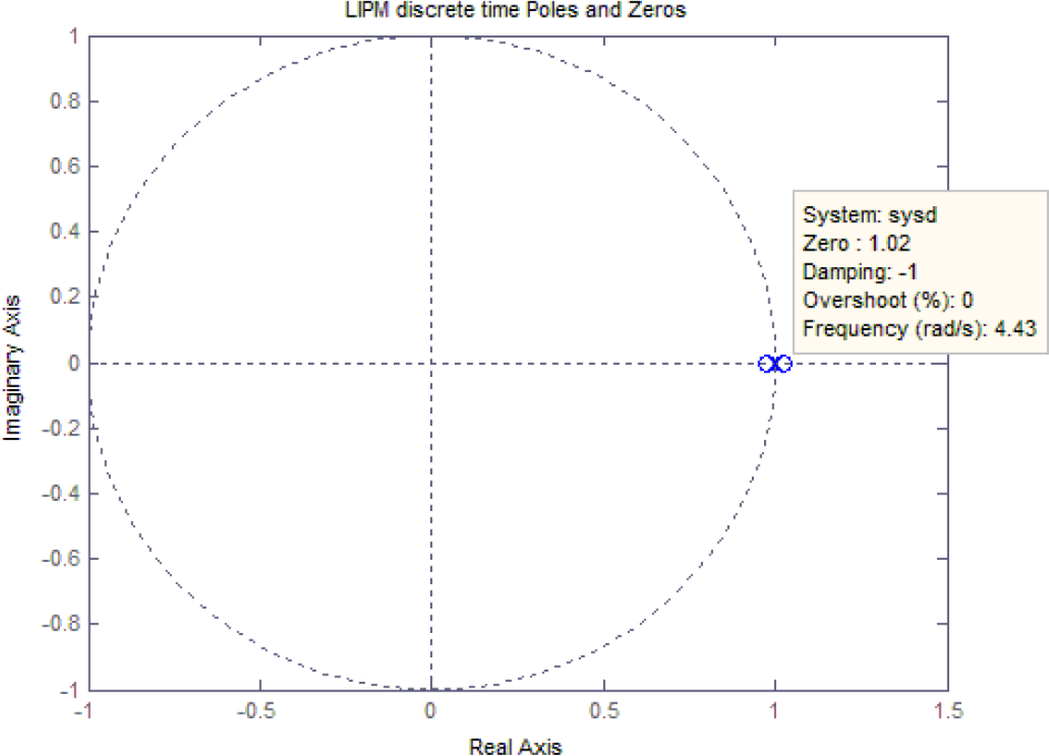
Discrete time poles zeros plot.
6. Augmented MPC State-Space Model with Embedded Integrator
Model predictive control (MPC) is designed based on a mathematical model of the plant system. In this paper, a state-space model is used in the tracking system design. The current time state variables are used to perform the predicting ahead operation [10]. The state-space model of the bipedal robot is presented in this section.
6.1 The Augmented 4Model Predicted Control (AMPC) Model
The proposed AMPC model used in this paper is an augmented state-space model with an embedded integrator. The set of equations (5.20) is re-written into the standard state-space form:
where xD is the discrete-time state variable (CoM), u is the discrete-time control input variable (jerk) and yD is the discrete-time tracked ZMP output. To include an integrator, taking a different operation on both sides of (6.1), yields:

The difference in the state variable and the difference in the control variable can be denoted by:
and define a new state variable vector. This yields the augmented state-space model [10]:

Where OD = [0 0 0] is the dimension of the state variable. The triplet (A, B, C) is the augmented model.
6.2 Prediction of CoM (the state) and ZMP (the output variable)
The system jerk (the control trajectory) is denoted as:

Where Nc is the control horizon, used to capture the future control system jerk trajectory. Where Np is the length of the prediction horizon optimization window. The future CoM state variables are predicted for Np samples. Denote the future CoM state variables as:

Where x(ki + m|ki) is the predicted state variable at (ki + m) with the given current plant information x(ki). The control horizon Nc is chosen to be Nc ≤ Np to the prediction horizon Np. All the predicted variables are in terms of current state variable information x(ki) and the future control parameters Δu(ki + j), where j = 0,1,2, …. Nc − 1. Define the following vectors:
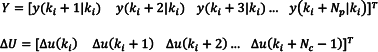
The dimensions of Y and U are Np and Nc respectively. By rearranging the parameters into matrix form:
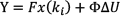
where

and

6.3 ZMP Tracking and Optimization
This optimization process is then translated to find an optimal control vector U such that the error between the input reference ZMP set-point trajectory and the CoM output trajectory is minimized. The vector that contains the set-point data information is written as:
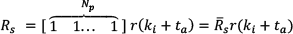
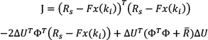
where ta is the adjustable look forward time-shift constant. The cost function J is defined as:

Where the first term is linked to the objective of minimizing the errors between the predicted ZMP output and the reference ZMP set point, and the second term reflects the consideration given to the rate of change in the system jerk ΔU when the objective function J is made as small as possible. The diagonal matrix R̅ = rwINc×Nc(rw≥0) is used as a tuning parameter to improve the closed-loop performance. For the case where rw = 0, the goal would be solely to make the ZMP error (Rs – Y) T (Rs – Y) as small as possible. For the case of a large rw, the cost function is interpreted, as it is carefully consider how large the rate of change in the system jerk ΔU might be and cautiously reduce the ZMP error. To determine the optimal ΔU, which minimizes J, substitute Equation (6.8) into (6.9). J is expressed as:
The necessary condition of the minimum J is derived:

By re-arranging Equation (6.11) and substituting (6.8) into (6.11), the optimal solution for the control signal is obtained:

As such, the optimal solution of the control signal is linked to the ZMP reference set-point signal and the state variable (CoM) by Equation (6.12).
6.4 Simulation
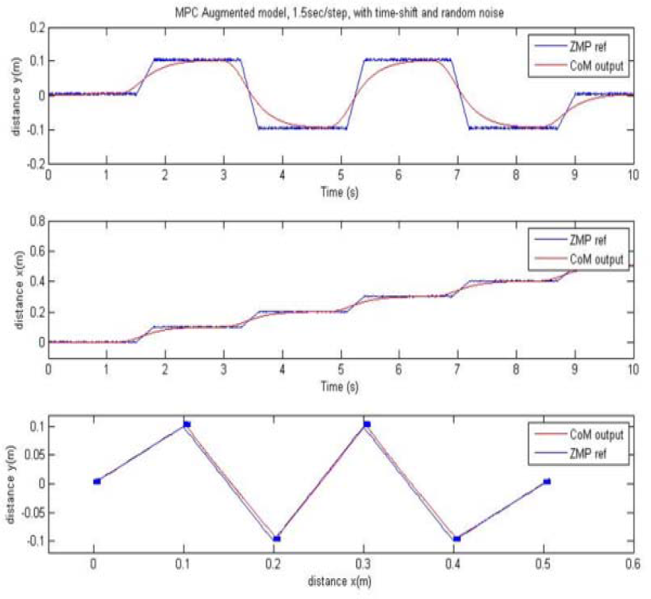
The initial simulation shows good tracking of the desired ZMP and CoM trajectory, as shown in Fig 6. The simulation parameters are given as follows: Nc = 100, Np = 300, ta = 80, rw = 10–5. The system is able to shift its desired CoM (red cure) to left/right feet during straight walking. Although AMP exhibits an initial undershoot (water-bed effect) due to the inherent characteristics of IPM because of the RHP zero, the CoM output (the desired signal in red) is smooth and it is able to closely follow the reference ZMP (blue waveform) trajectory. Figure 20 shows that the jerk in both the X and Y direction is minimized to zero by the cost function.

The jerk reduced to zero.
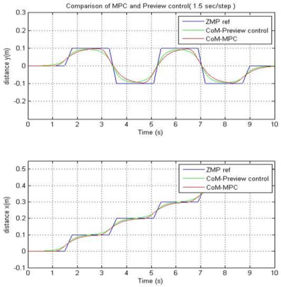
6.5 Comparison of AMPC with Preview method
With a closer examination of the CoM trajectory produced using the AMPC tracking, as depicted in Figure 20, it can be seen that the CoM curve (in red) moves slowly toward the reference ZMP curve (in blue). This can be interpreted as the controller trying to reduce the jerk and impact force during swing foot landing and cautiously reduce the ZMP error. As a result, the weight of CoM transfers from the supporting foot to the landing foot (new supporting foot) during the double support phase (DSP) is slow and gentle. In comparison with the preview control technique [1], which produces a symmetrical sinusoidal waveform (in green), the AMPC algorithm produces a truncated sinusoidal trajectory during swing foot landing due to its ‘soft landing, fast take off characteristics. The other advantages of using the AMPC model is that the optimization process does not need to solve the Riccati equation and the optimization window can be easily adjusted to fine-tune the system response. Since AMPC uses a recursive iteration method, with continuing improvement in computer hardware and software architecture, this in turn reduces system-processing time and therefore, it is possible to implement it in AMPC real-time.
6.6 Augmented MPC model with noise
One of the key features of AMPC predictive control is the ability to handle constraints in the design. To check the robustness of the AMPC model in tracking the desired ZMP, random noise (±0.05m) is added to the reference ZMP waveform. The simulation results are as depicted in Figure 21. This shows that the AMPC model is still able to produce a good track output in a noisy environment.
AMPC and Preview control plot.
An observer may be in a situation where either the state variable x(ki) is too noisy or not measurable. The robot state x(ki) is estimated by an observer of the form:

6.7 Observer-based Predictive Control
The predictive control law is similar to Equation (6.10), to find ΔU by minimizing:
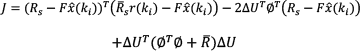
The optimal solution is obtained as:

The optimal solution for Δu(ki) at time ki, from (6.15) is:

The closed-loop characteristic equations and the Eigenvalues of the closed-loop system are obtained as follows:

The close loop observer error equation is:

Where x˜(k) = x(k) – ◯(k), (6.17) can be rewritten as:

Combining (6.18) and (6.19) leads to:

The characteristic equation of the close-loop state space system is obtained as:


This means that the robot closed-loop model and the state estimator have two independent characteristic equations:
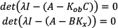
As such, one can design the predictive control law and the observer separately.
6.8 Walking on stairs and slope
The AMPC algorithm can also be applied to control a robot walking on a slope, on stairs and clearing an obstacle, as depicted in Figure 22 (a) and (b). The joints' trajectory for straight walking for two steps on flat surface is shown in Figure 23.
AMPC trajectory tracking with noisy input.

Robot walking on different surface
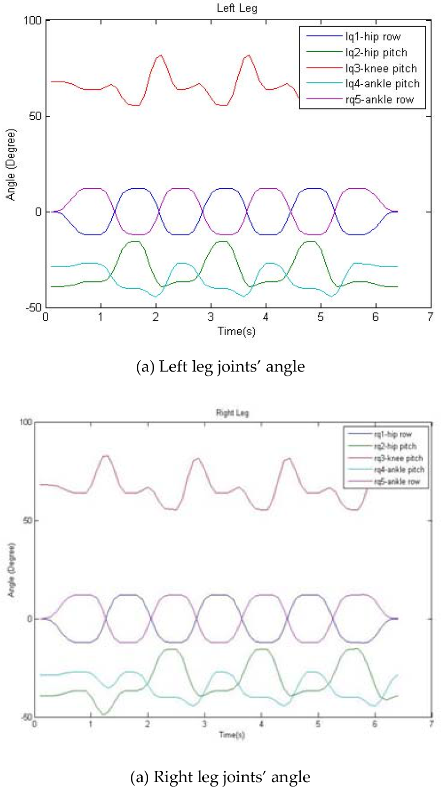
The robot joints' trajectories (walking two steps on a flat surface).
6.9 Step over obstacle
Controlling the robot to step over an obstacle without tipping over is quite a challenging task. The general procedure is to first define the constraints on the leg joints limited by its leg structure and kinematics, followed by formulating the balance and collision-free constraints and finally deriving the mathematical models. The stepping over an obstacle trajectory can be achieved by using a set-point method, a polynomial function or optimal path search algorithms. The motion sequences are depicted in Figure 24. The eight basic step sequences are outline as follows:
double support, robot in initial posture, ready to step over obstacle.
double support, the robot move its pelvis (CoM) to the supporting leg.
single support, the robot lifts its swing leg, moves the swing foot over the obstacle.
double support, robot lands its swing leg on the other side of the obstacle.
double support, the robot moves it pelvis (CoM) toward the front support leg.
single support, the robot lifts its rear leg, swing it upward and over to clear the obstacle.
double support, robot moves back to initial posture.
double support, ready for next action.

Step over obstacle sequences
7. Conclusion
In this paper, the sensory feedback system and the control algorithm structure for a bipedal robot TPinokio is presented. A new control algorithm with an AMPC method is also proposed and the simulation results are presented and compared with the preview control method. With a trade off in sampling and update rate, it is possible to implement the control algorithm with on-line updates close to real-time by using a high-speed computer. The current work implements this algorithm with an NI PXI real-time system. Future work will combine the discrete-time AMPC with the Laguerre function and the observer [5] to further enhance and refine the tracking algorithm and the joints' trajectory in order to reduce the effect of the undershoot water-bed phenomenon.
For more details and updates on the development progress, readers may visit the website www.tpinokio.com.