Sage Journals: Discover world-class research

Abstract

Stable bipedal walking is one of the most important components of humanoid robot design, which can help us better understand natural human walking. In this paper, to study gait selection and gait transition of efficient bipedal walking, we proposed a dynamic bipedal walking model with an upper body, flat feet and compliant joints. The model can achieve stable cyclic motion with different walking gaits. The hip actuation and ankle stiffness behavior of the model are quite similar to those of human normal walking. In simulation, we studied the influence of hip actuation and ankle stiffness on walking performance of each gait. The effects of ankle stiffness on gait selection are also analyzed. Gait transition is realized by adjusting ankle stiffness during walking.

Keywords

Gait selection gait transition passive dynamic walking humanoid robots joint stiffness

1. Introduction

Stability guaranteed bipedal walking is one of the keys but also one of the more challenging components of humanoid robot design. Study on bipedal walking can help us better understand the principle of the sophisticated human walking and build efficient bipedal walking prototype. Most industrial bipedal robots were realized based on the trajectory-control approach [1]. By controlling joint angles precisely, the zero moment point (ZMP) is kept within the convex hull of the supporting area [2]. These actively controlled robots can perform various walking gaits and complete different tasks. However, this kind of bipedal robots often walk with low energetic efficiency and unnatural gaits.

Different from the actively controlled walking, passivity-based dynamic bipedal walking may not reach equilibrium at every moment during motion, but can realize stable cyclic locomotion. Passive dynamic walking [3] has been presented as a possible explanation for the efficiency of the human gait, which showed that a mechanism with two legs can be constructed so as to descend a gentle slope with no actuation and no active control. Several studies reported that these kinds of walking machines work with reasonable stability over a range of slopes [3], [4], [5] and on level ground with kinds of actuation added [6], [7]. Most studies of passivity-based dynamic walking are based on the Simplest Walking Model proposed by [8] and extended work by [9]. Recently, several flat-foot dynamic walking models are established to further study the bipedal locomotion [10], [11], [12], [13], [14]. Compared with the actively controlled walking, passivity-based walking achieves higher efficiency and performs more natural walking gait, which shows a remarkable resemblance to human normal walking [6].

However, the bipedal robots based on passive dynamic walking are often of poorly practical use. Most of these walkers are limited to one predefined walking pattern. The walking velocity and step length are fixed during the locomotion. People are able to perform various walking gaits at different speeds and step lengths with high efficiency. Inspired by natural human walking, existing studies have made efforts to introduce adaptable compliance to passivity-based bipedal walking, to improve the versatility and achieve multi-gait walking with low energy consumption. Hobbelen et al. showed that ankle stiffness is important for dynamic walking with flat feet [12]. Wang et al. studied the effects of the ankle stiffness on motion characteristics of flat-foot dynamic walkers [13], [14]. However, these studies focused on only one predefined walking gait. To study multiple gaits of passive bipeds, Owaki et al. proposed a two-link passive bipedal model with hip torsional spring and leg springs, and investigated the distribution of different gaits with different hip stiffness and leg stiffness [15]. Geyer et al. found that both running and different walking gaits can be realized by the bipedal model with compliant legs [16]. Nevertheless, these two studies used relatively simple models with point feet and did not analyze the influence of ankle joint compliance in dynamic walking. Our previous studies realized multiple dynamic walking gaits of a passivity-based biped and analyzed the motion characteristics of each gait [17], [18].

To investigate gait selection and gait transition of dynamic bipedal walking with high efficiency and various gaits, in this study, we propose a seven-link bipedal walking model with an upper body, compliant knee joints and ankle joints, flat feet and hip actuation. Different walking gaits are obtained by changing hip actuation and ankle stiffness. We compare the performance of different walking gaits and study the effects of hip actuation and ankle stiffness on gait selection. Moreover, the model realizes walking gait transition in real-time through adjusting the ankle joint stiffness during walking. The investigation in this study reveals the effects of ankle joint stiffness on generating different walking gaits and on walking gait transition. The results could further our understanding of human walking and provide guidance in building efficient multi-gait humanoid robots.

The paper is organized as follows. The modeling of the proposed biped is described in detail in Section II. In Section III, we indicate the sequence of the walking phases of each gait and the actuation mode. Section IV shows the experimental results on the proposed model and relevant analysis. We conclude in Section V.

2. Dynamic Bipedal Walking Model

2.1 Bipedal model with flat feet and compliant joints

In this study, we propose a passivity-based bipedal walking model that is more close to human beings. The model includes an upper body, two thighs, two shanks and flat feet. As shown in Fig. 1, the two-dimensional model consists of two rigid legs interconnected individually through a hinge with a rigid upper body (mass added stick) connected at the hip. Each leg includes thigh, shank and foot. The thigh and the shank are connected at the knee joint, while the foot is mounted on the ankle with a torsional spring. A point mass at hip represents the pelvis. The mass of each leg and foot is simplified as point mass added on the Center of Mass (CoM) of the corresponding stick. Similar to [19], a kinematic coupling has been used in the model to keep the upper body midway between the two thighs. Specifically, knee joints and ankle joints are modeled as passive joints that are constrained by torsional springs. To simplify the motion, we have several assumptions, including: 1) each stick suffers no flexible deformation; 2) there is no damping or friction in the hip joint and knee joints; 3) the friction between the walker and the ground is large enough, which means the flat feet do not deform or slip; 4) all strikes are modeled as instantaneous, fully inelastic impacts where no slip or no bounce occurs. The bipedal walker travels forward on level ground with hip actuation.

Figure 1.

Dynamic bipedal walking model with flat feet and compliant ankle joints.

The stance leg keeps contact with the ground while the swing leg pivots about the constraint hip. When the flat foot strikes the ground, there are two impulses, “heel-strike” and “foot-strike”, representative of the initial impact of the heel and the following impact as the whole foot strikes the ground [13]. The shank of the stance leg is always locked and the whole leg can be modeled as one rigid stick, while the knee joint of the swing leg will release the shank immediately after foot-strike. The knee joint will be locked when the shank swings forward to a relatively small angle to the thigh.

We suppose that the x-axis is along the ground while the y-axis is vertical to the ground upwards. The configuration of the walker is defined by the coordinates of the point mass on the hip joint and several angles, including the angles between the vertical axis and each thigh and shank, the angle between the vertical axis and the upper body and the angles between the horizontal axis and each foot (see Fig. 1 for details), which can be arranged in a generalized vector q = (x_h, y_h, θ₁, θ₂, θ₃, θ_2s, θ_1f, θ_12f)'. The superscript' means the transposed matrix (the same in the following paragraphs). The positive directions of all the angles are counter-clockwise. Note that the dimension of the generalized coordinates q in different phases may be different. When the knee joint of the swing leg is locked, the freedom of the shank is reduced and the angle θ_2s is not included in the generalized coordinates. Consequently, the dimensions of mass matrix and generalized active force are also reduced in some phases.

2.2 Walking dynamics

In the following paragraphs, we will focus on the Equation of Motion (EoM) of the bipedal walking dynamics of the proposed model. The model can be defined by the rectangular coordinates r, which can be described by the x-coordinate and y-coordinate of the mass points. The walker can also be described by the generalized coordinates q as mentioned before (suppose leg 1 is the stance leg):

q = (x_{h}, y_{h}, θ_{1}, θ_{2}, θ_{3}, θ_{2 s}, θ_{1 f}, θ_{2 f})'

(1)

We define matrix J as follows:

J = d r / d q

(2)

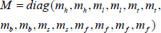
Thus J transfers the independent generalized coordinates q̇ into the velocities of the rectangular coordinates ṙ. The mass matrix in rectangular coordinate r is defined as:

\begin{array}{l} M = d i a g (m_{h}, m_{h}, m_{l}, m_{l}, m_{t}, m_{t}, \\ m_{b}, m_{b}, m_{s}, m_{s}, m_{f}, m_{f}, m_{f}, m_{f}) \end{array}

(3)

We denote F as the active external force vector in rectangular coordinates. The constraint function is marked as ξ(q), which is used to maintain foot contact with ground and detect impacts. Note that ξ(q) in different walking phases may be different since the contact conditions change. Each component of ξ(q) should keep zero to satisfy the contact condition.

The contact of the stance foot is modeled by one ground reaction force (GRF) along the floor and two GRFs perpendicular to the ground acted on the two endpoints of the foot, respectively. If one of the forces perpendicular to the ground decreases below zero, the corresponding endpoint of the stance foot will lose contact with ground and the stance foot will rotate around the other endpoint.

We can obtain the EoM by Lagrange's equation of the first kind:

M_{q} {\ddot{q} = F}_{q} + Φ {' F}_{c}

(4)

ξ (q) = 0

(5)

where $\frac{\partial ξ}{\partial q} {\dot{q}}^{+} = 0$ . F_c is the generalized constraint force vector. M_q is the mass matrix in the generalized coordinates q:

M_{q} = J' M J

(6)

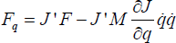
F_q is the active external force in the generalized coordinates:

F_{q} = J' F - J' M \frac{\partial J}{\partial q} \dot{q} \dot{q}

(7)

Equation (5) can be transformed to the following equation:

Φ \ddot{q} = - \frac{\partial (Φ \dot{q})}{\partial q} \dot{q}

(8)

Then the EoM in matrix format can be obtained from Equation (4) and Equation (8):

(\begin{matrix} M_{q} & - Φ' \\ Φ & 0 \end{matrix}) (\begin{matrix} \ddot{q} \\ F_{c} \end{matrix}) = (\begin{matrix} F_{q} \\ - \frac{\partial (Φ \dot{q})}{\partial q} \dot{q} \end{matrix})

(9)

The equation of strike moment can be obtained by integration of Equation (4):

M_{q} {\dot{q}}^{+} = M_{q} {\dot{q}}^{-} + Φ' I_{c}

(10)

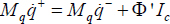
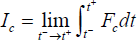
where q̇⁺ and q̇⁻ are the velocities of generalized coordinates just after and just before the strike, respectively. Here, I_c is the impulsive acted on the walker which is defined as follows:

I_{c} = \lim_{t^{-} \to t^{+}} \int_{t^{-}}^{t^{+}} F_{c} d t

(11)

Since the strike is modeled as a fully inelastic impact, the walker satisfies the constraint function ξ(q). Thus the motion is constrained by the followed equation after the strike:

\frac{\partial ξ}{\partial q} {\dot{q}}^{+} = 0

(12)

Then the equation of strike in matrix format can be derived from Equation (10) and Equation (12):

(\begin{matrix} M_{q} & - Φ' \\ Φ & 0 \end{matrix}) (\begin{matrix} {\dot{q}}^{+} \\ I_{c} \end{matrix}) = (\begin{matrix} M_{q} {\dot{q}}^{-} \\ 0 \end{matrix})

(13)

3. Bipedal Walking Gaits

3.1 Walking sequence

Based on the proposed bipedal walking model, we analyzed the possible walking gaits in this section. Different from the existing studies, the series of walking phases is not predefined in this study. The dynamic switching of the walking phases is more close to that of real human walking.

The walking sequence of the flat-foot walker is more complicated than that of the round-foot walker [10], [14]. Each foot has three contact cases: foot contact, heel contact and toe contact. Thus there appear several sub-streams in the walking sequence, which is different from the motion of round-foot models and point-foot models (see Fig. 2). Note that the sequence in Fig. 2 has several sub-streams. One walking step may not include all these phases. Moving to which phase at the bifurcation point is based on the contact force.

Figure 2.

Walking sequence of the passivity-based biped with flat feet and compliant ankle joints. The walking sequence has several sub-streams which indicate different gaits.

In this study, different walking phases are distinguished by the constraint conditions. For example, in Fig. 2, the whole foot of the trailing leg maintains contact with the ground in phase H, while only the toe of the trailing leg is fixed on the ground in phase I. Thus phase H and phase I have different constraint conditions. Fig. 2 shows all the possible walking phases of the proposed model in one walking step. In this paper, we denote “walking gait” as the sequence of certain walking phases under specific order. For example, cyclic motion with the sequence “A → B → C → D → F → H → K → A” is one walking gait, and the periodic walking with the sequence “A → B → C → D → F → H → I → L → A” is another walking gait. The bipedal walking may switch dynamically between different walking gaits. The walker may also change walking velocity and step length during the same gait, which is considered as “walking pattern transition” in this study.

3.2 Walking phases

As shown in Fig. 2, phase A is the push-off phase, the initial phase of certain gaits. In this phase, the trailing foot rotates around the toe with a push-off effect. The foot will lift up when the ground force acted on the toe decreases to zero, which means that the toe loses contact with ground. Then the walker will move to phase B.

In phase B, C, D and E, the swing leg of the walker swings freely with no contact with the ground. The shank of the swing leg is released in phase B. When the shank of the swing leg swings to a relatively small angle to the thigh, the knee joint is locked. There is an impact between the shank and the thigh of the swing leg in phase C. Then the shank and the thigh are supposed to be constrained in a straight line and the model moves to phase D. If the heel of the trailing foot loses contact with the ground before the leading foot strikes the ground, the walker will move to phase E, otherwise the walker will move to phase F.

Phase F and G are heel-strike phases. There is an impact between the swing leg and the ground when the heel of the swing leg contacts the ground. The difference between the two phases is the constraint condition of the trailing foot. After the strike, the walker moves to phase H or I.

After heel-strike, the foot of the leading leg rotates around the heel. In phase H, the whole foot of the trailing leg maintains contact with the ground. If the contact force acted on the heel of rear leg decreases to zero, the model will move to phase I. The toe of the rear leg and the heel of the fore leg maintain contact with the ground in phase I. If the contact force acted on the toe of the trailing leg decreases to zero, the model will move to phase J, in which the whole walker has contact with the ground only at the heel of the leading leg.

After foot rotation phases, the walker moves to foot-strike phases, including phase K, L and M. There is an impact between the whole foot of the leading leg and the ground. The difference among the three phases is the constraint of the trailing leg. After foot-strike, the stance leg and the swing leg will be swapped and another walking cycle will begin.

3.3 Walking gaits

According to the walking sequence discussed above, the dynamic bipedal walking model in this study has five possible gaits as follow:

Gait 1: “A → B → C → D → F → H → K → A”. The whole foot of the stance leg keeps contact with ground till the foot-strike of the swing leg occurs. This gait often has a very short step length.

Gait 2: “A → B → C → D → F → H → I → L → A”. The heel of the stance leg loses contact with ground before the foot-strike of the swing leg occurs. The step length of this gait is relatively small.

Gait 3: “B → C → D → F → H → I → J → M → B”. The whole foot of the stance leg leaves ground before the foot-strike of the swing leg. This gait is quite rare since it has no push-off phase.

Gait 4: “A → B → C → D → E → G → I → L → A”. The heel of the stance leg loses contact with the ground before the heel-strike of the swing leg, which is called premature heel rise [20]. This gait often has a relatively large step length.

Gait 5: “B → C → D → E → G → I → J → M → B”. The heel of stance leg leaves ground before heel-strike of swing leg, while the whole stance foot loses contact with ground before the foot-strike of the swing leg occurs. This gait often appears in the large step length walking for stepping over small obstacles or pits.

Gait 1 with a short step length can be found in walking in a crowded queue. The step length is confined in a small range. Gait 2 is quite similar to gait 1. Previous studies have demonstrated that the push-off of the trailing leg begins slightly before double support in human normal walking [21], thus gait 4 is most close to real human walking among all the gaits above. Gait 3 and gait 5 are rare since they have no push-off phases.

Not that the walking sequence shown in Fig. 2 is an ideal case according to the multi-rigid body mechanics. Some of the walking gaits (for example, gait 3 and gait 5 which not include the push-off phase) in the sequence are rarely found in real human walking. Thus we ignore these gaits in this paper for their atypical performance. The three most commonly walking gaits (gait 1, gait 2 and gait 4) will be analyzed in detail in Section IV.

3.4 Actuation Mode

We add a piecewise constant hip torque to actuate the walker to travel forward on level ground. The hip torque may be different in different phases. The torque is relatively larger in push-off phase and double-support phase to actuate the swing foot to leave ground and compensate the energy loss at heel-strike, respectively, and is near zero in the freely swing phases based on the fact that the muscles of the swing leg are generally silent [22].

In the simulation, stable cyclic walking is searched for various combination of hip actuation and ankle stiffness. The hip torques of the representatives of the five gaits are shown in Fig. 3.

Figure 3.

The hip actuation patterns of the five gaits. Gait 1 and gait 2 have the same patterns. The hip torque of gait 4 is different from gait 1 and gait 2 only in the double-support phase. Since gait 3 and gait 5 do not include push-off phase, the corresponding parts are absence in the figure.

Torsional springs are added at ankle joints to represent ankle stiffness. Several studies indicate that ankle behavior in human walking is quite similar to that of a torsional spring [23], [24]. The ankle stiffness in human walking varies in one step [25]. In this study, we set different values of ankle stiffness during the stance phase, which shows a large resemblance with human normal walking (see Fig. 4). Similar approaches have been used in [12].

Figure 4.

Comparison of ankle behavior of human normal walking and the proposed model. (a) shows the torque-angle relationship in ankle joint of human normal walking, adapted from Frigo et al [23]. Ankle angle is the relative angle between the shank and the foot. y-axis is the ankle joint torque. (b) shows the torque-angle relationship in the ankle joint of the proposed model. O (the origin point): Heel-strike; O → A: Toe-down phase; A → O: Foot-flat phase (the leg is before mid-stance. The ankle stiffness is Ka); O → B: Foot-flat phase (the leg has passed mid-stance and the ankle stiffness has a larger value Kb.); B → C: Heel-up phase. The ankle stiffness returns to Ka. The line BC is parallel to the line AO; C → O: Swing phase, the foot is reset to the equilibrium position.

In our bipedal walking model, the ankle stiffness has a larger value when the stance leg has passed the ground normal during the foot-flat phase. During the rest of the stance, the ankle stiffness is lower. In toe-down, foot-flat and swing phases (O → A, A → O and B → C in Fig. 4(b)) the ankle joint reaches equilibrium position when the leg is perpendicular to the foot. The equilibrium position has a deviation in heel-off phase (O → B in Fig. 4(b)). The ankle torque changes continuously at the switching of ankle stiffness, which means that the switching does not bring additional energy. The foot is supposed to be constrained vertically to the shank to avoid oscillation during swing phase. The ankle does a amount of net work during one step as shown by the hatched area in Fig. 4(b), which is taken consider into the calculation of energetic efficiency.

Both the hip actuation mode and the ankle behavior are predefined with no active control during the walking motion.

4. Experimental Results

In this section, we show the simulation experiments to investigate the effects of hip actuation and ankle stiffness on gait selection and gait transition of the proposed dynamic walking biped. All simulations and data processing were performed using Matlab 7 (The Mathworks, Inc., Natick, MA).

The parameter values used in the analysis are specified in Table 1. All masses and lengths are normalized by total mass of the model and the leg length respectively.

Table 1.

Parameter values in simulations.

Parameter	Value
leg mass m_l	0.1538
thigh mass m_t	0.1077
shank mass m_s	0.0461
foot mass m_f	0.0355
body mass m_b	0.355
hip mass m_h	0.2663
leg length l	1
thigh length l_t	0.55
shank length l_s	0.45
foot length l_f	0.25
upper body length l_b	0.75
distance from hip joint to CoM of thigh c_t	0.2750
distance from knee joint to CoM of shank c_s	0.2250
distance from ankle joint to CoM of foot c_f	0.0250
distance from hip joint to CoM of upper body c_b	0.3750

Periodic walking of all the five gaits described in Section 3. C are found with the parameter values in Tab. 1. The leg trajectories of the gaits are shown in Fig. 5. In the rest of this section, we focus on the motion characteristics of gait 1, gait 2 and gait 4, since gait 3 and gait 5 are quite rare in real human walking as mentioned above.

Figure 5.

The leg trajectories of the five walking gaits. The closed curve in each sub-figure indicates the relationship between the angle of the thigh and the angular velocity of the thigh during cyclic motion. The hip actuation of each gait is set as Fig. 3. The ankle stiffness of each gait is chosen as follows: (a) gait 1, Ka is 20Nm/rad, Kb is 36Nm/rad; (b) gait 2, Ka is 50Nm/rad, Kb is 90Nm/rad; (c) gait 3, Ka is 93Nm/rad, Kb is 100Nm/rad; (d) gait 4, Ka is 35Nm/rad, Kb is 95Nm/rad; (e) gait 5, Ka is 40Nm/rad, Kb is 95Nm/rad.

4.1 Effects of hip actuation and ankle stiffness on walking performance

For the analysis of the energy loss at heel-strike of different gaits, we studied the walking performance (energy efficiency, walking velocity and step length) of gait 1, 2 and 4 with variant hip torques in double-support phases. Fig. 6 shows the results. The three gaits have the same hip torques in push-off phases.

Figure 6.

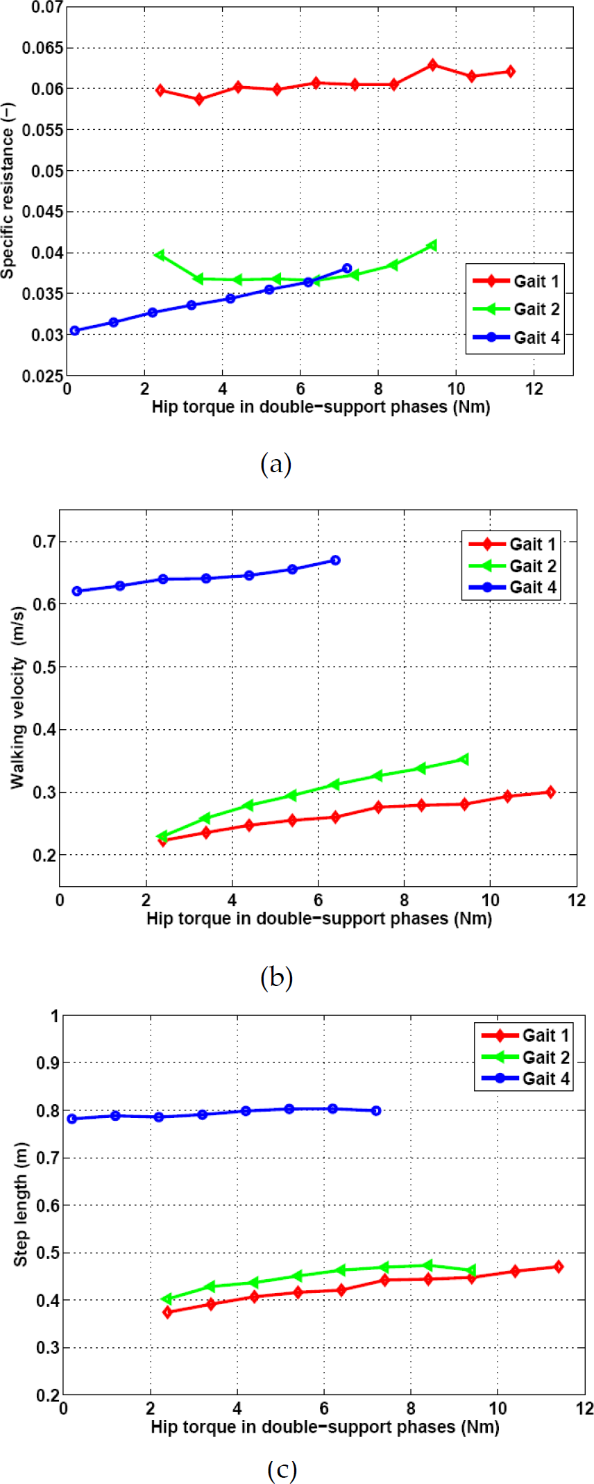
The effects of hip torques in double-support phases on walking performance of gait 1, gait 2 and gait 4. (a), (b) and (c) indicate the energy efficiency, walking velocity and step length with variant hip torques, respectively.

Similar to previous studies [6], [7], the energy efficiency of the proposed model in this study is evaluated by the dimensionless ratio “specific resistance”:

S_{r} = \frac{E}{M g L}

(14)

where E is the energy consumption during walking, M is the total mass of the walker, g is the gravitational acceleration, and L is the distance the walker traveled.

Fig. 6 (a) shows the specific resistance of the three gaits. One can find that gait 4 is the most efficient gait, since the specific resistance of gait 4 is minimal in most cases. Contrarily, the efficiency of gait 1 is the lowest. Fig. 6 (b) and (c) indicate that gait 4 has the largest walking velocity and step length, while gait 1 is the most slow gait with smallest step length. Fig. 6 also shows that stable periodic motions of gait 1 and gait 2 are often found when the hip torques are relatively large, while cyclic walking of gait 4 can be found with smaller hip actuation, which demonstrates that the energy loss at heel-strike of gait 4 is the smallest. It means the trailing leg begins push-off before the heel-strike of the leading leg can reduce the energy loss, which is consistence with [26]. Thus the gait which is most close to real human walking is the most efficient one. Moreover, the results in Fig. 6 show that both the walking velocity and step length increase with increasing hip actuation, while the hip torque only has a minimal influence on energy efficiency.

Fig. 7 shows the effects of ankle stiffness on the energy efficiency, walking velocity and step length of gait 1. The efficiency is relatively low when Ka is small (e.g. Ka is 20Nm/rad). Increasing Kb results in decreasing efficiency. The effects of the ankle stiffness on step length are similar to those on the energy efficiency. In general, both the velocity and step length decreases with increasing Ka and increases with increasing Kb.

Figure 7.

The relationship between ankle stiffness and walking performance of gait 1. (a), (b) and (c) indicate the energy efficiency, the walking velocity and the step length, respectively.

In gait 2, the bipedal model walks with poor energy efficiency with small Ka (e.g. Ka is 55Nm/rad). However, the relationship between efficiency and Kb is not monotonous if Ka increases to a relatively large value. For a given Ka, there exists an optimal Kb in the view of energy efficiency. Within the range of ankle stiffness shown in Fig. 8, the most efficient walking (the specific resistance is 0.036) is achieved when Ka is 85Nm/rad and Kb is 120Nm/rad. The tendencies of velocity and step length with variant ankle stiffness of gait 2 are similar to those of gait 1.

Figure 8.

The relationship between ankle stiffness and walking performance of gait 2. (a), (b) and (c) indicate the energy efficiency, the walking velocity and the step length, respectively.

In gait 4, the range of Kb is quite small. The effects of Ka on walking performance of gait 4 are similar to those of gait 1 and gait 2, as shown in Fig. 9. With increasing Ka, the efficiency of the walker increases, while the velocity and the step length decrease.

Figure 9.

The relationship between ankle stiffness and walking performance of gait 4. (a), (b) and (c) indicate the energy efficiency, the walking velocity and the step length, respectively.

4.2 Gait distribution

To further investigate the effects of ankle stiffness on gait selection, we discussed the distribution of gait 1, gait 2 and gait 4 among different ankle stiffness.

Our experimental results indicate that ankle stiffness plays an important role in gait selection. Different ankle stiffness may result in different gaits with the same mechanical parameters. Fig. 10 shows the distribution of the three gaits. Dynamic walking with both lower Ka and lower Kb converges to gait 1, while larger Ka and Kb lead to gait 2. The cyclic walking in gait 4 is found when Ka is relatively small and Kb is large. There are also some “mixed” regions in the Ka-Kb plane, where the bipedal walker performs hybrid gaits. For example, “Gait 1 and Gait 2” in Fig. 10 refers to the following cases: 1) Cyclic motions both with gait 1 and with gait 2 are found at the same ankle stiffness. The initial conditions of the two gaits are different; 2) Gait 1 and gait 2 alternatively appear in different steps of the walking.

Figure 10.

Distribution of different walking gaits in the Ka-Kb plane.

Fig. 11 shows the distribution of different walking gaits in velocity-step length plane. There is certain positive correlation between walking velocity and step length. In general, larger step length corresponds to faster walking. Relevant biological research indicates that human normal walking approximately satisfies the relation “step length ~ velocity^0.42” [26], as shown by the dashed line in Fig. 11. The velocity-step length relation of the proposed model is similar to that of human beings, which demonstrates that the dynamic walking in this study reflects the real human walking to some extent. Compared with gait 1 and gait 2, the cyclic motions in gait 4 are more close to the dashed line in Fig. 11, which also supports that gait 4 is more similar to human normal walking than other gaits.

Figure 11.

Distribution of different walking gaits in the velocity-step length plane. The dashed line is the relationship between walking velocity and step length of human normal walking.

Fig. 12 is the distribution of different walking gaits in the velocity-efficiency plane. Efficiency is measured by specific resistance. Generally, gait 1 has the lowest efficiency. Gait 2 and gait 4 are more efficient. The step length of gait 1 is the smallest, while gait 4 has the largest step length.

Figure 12.

Distribution of different walking gaits in the velocity-specific resistance plane.

4.3 Gait transition

In this sub-section, we focused on walking transitions between different patterns or gaits. Based on the analysis above, walking pattern transition and walking gait transition are realized through adjusting ankle stiffness during motion.

Here we show an example of walking pattern transition in gait 2 and another example of walking gait transition from gait 1 to gait 2, to illustrate walking transition in real-time through tuning ankle stiffness.

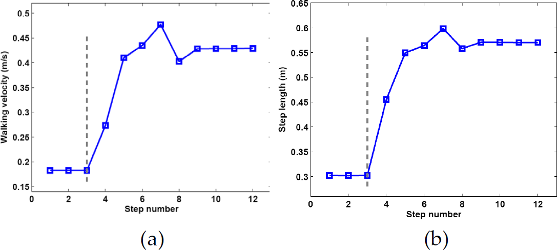
Fig. 13 shows the trajectory of walking pattern transition in gait 2. In the beginning, the ankle stiffness is: Ka =80Nm/rad, Kb = 105Nm/rad. The initial states are set as the initial conditions of the stable periodic walking under this ankle stiffness. At the end of the third step, the ankle stiffness starts to change. At the end of the seventh step, the ankle stiffness reaches the target value: Ka = 70Nm/rad, Kb = 115Nm/rad. From Fig. 13, one can observe that the step length begins to decrease gradually at the fourth step. Finally the walking pattern converges to the cyclic motion of the new ankle stiffness. Fig. 14 is the leg trajectory of the walking pattern transition. The trajectory transitions from one closed curve to another closed curve gradually. Fig. 15 shows the change of walking velocity and step length of the transition. The change starts at the fourth step, and the performance becomes stable at about the eleventh step.

Figure 13.

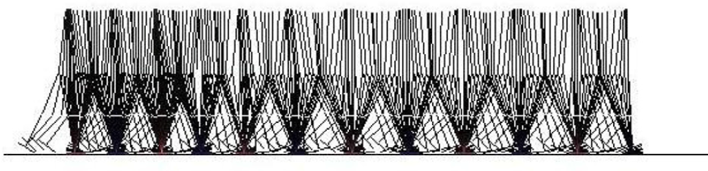
Stickgram of walking pattern transition in gait 2. The ankle stiffness is changed from Ka =80Nm/rad, Kb =105Nm/rad to Ka =70Nm/rad, Kb = 115Nm/rad.

Figure 14.

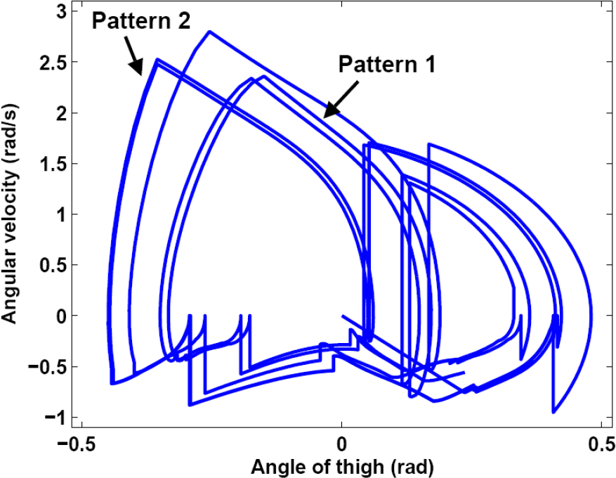
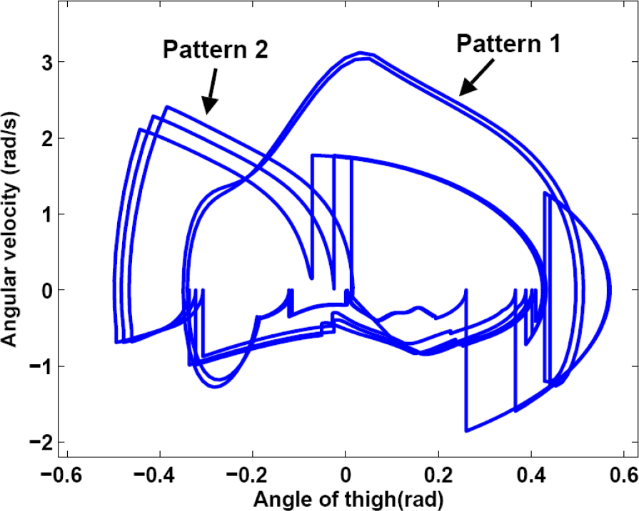
Leg trajectory of walking pattern transition in gait 2. The ankle stiffness is changed from Ka = 80Nm/rad, Kb = 105Nm/rad to Ka = 70Nm/rad, Kb = 115Nm/rad. Pattern 1 is the initial pattern, and pattern 2 is the target pattern.

Figure 15.

The velocity and step length of walking pattern transition in gait 2. The ankle stiffness is changed from Ka = 80Nm/rad, Kb = 105Nm/rad to Ka = 70Nm/rad, Kb = 115Nm/rad. The dashed line indicates the moment the transition begins. (a): the change of walking velocity; (b): the change of step length.

In the experiment of walking gait transition from gait 1 to gait 2, the ankle stiffness before and after transition are Ka = 65Nm/rad, Kb = 90Nm/rad (gait 1) and Ka = 60Nm/rad, Kb = 105Nm/rad (gait 2), respectively. The bipedal model walks stably with gait 1 at the beginning. The change of ankle stiffness starts at the end of the second step and ends at the end of the sixth step. Fig. 16, Fig. 17 and Fig. 18 are the stickgram, leg trajectory and the change of velocity and step length, respectively. The results of walking gait transition show similar performance to those of walking pattern transition. Compared with walking pattern transition, the change of leg trajectory in walking gait transition is more obvious. Not only the position and the size, but also the shape of the trajectory is changed during the transition.

Figure 16.

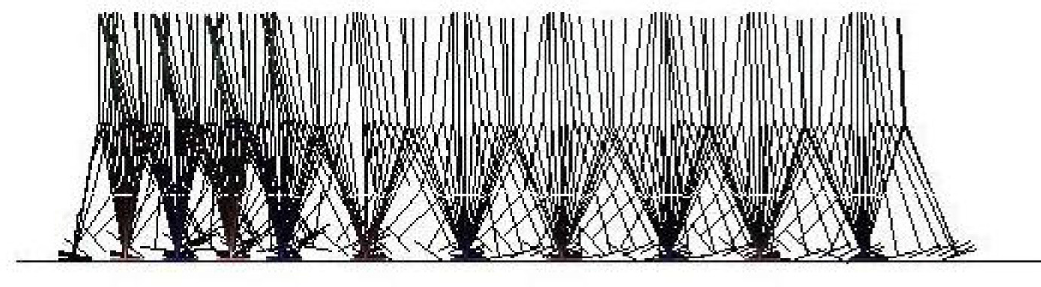
Stickgram of transition from gait 1 to gait 2. The ankle stiffness is changed from Ka = 65Nm/rad, Kb = 90Nm/rad to Ka = 60Nm/rad, Kb = 105Nm/rad.

Figure 17.

Leg trajectory of transition from gait 1 to gait 2. The ankle stiffness is changed from Ka = 65Nm/rad, Kb = 90Nm/rad to Ka = 60Nm/rad, Kb = 105Nm/rad. Pattern 1 is the initial pattern of gait 1, and pattern 2 is the target pattern of gait 2.

Figure 18.

The velocity and step length of transition from gait 1 to gait 2. The ankle stiffness is changed from Ka = 65Nm/rad, Kb = 90Nm/rad to Ka = 60Nm/rad, Kb = 105Nm/rad. The dashed line indicates the moment the transition begins. (a): the change of walking velocity; (b): the change of step length.

It is worth mentioning that the pattern transition and gait transition of the dynamic bipedal walking in this study are realized by adjusting the ankle stiffness, but not by changing the actuation torques directly. Thus the change of walking performance results from tuning the natural dynamics of the model, but not results from only controlling the external actuation. The approach in this paper is more close to real human walking.

5. Conclusion

In this paper, we have presented a dynamic bipedal walking model with flat feet and compliant ankle joints and proposed the sequence of walking phases with multiple gaits. The adopted hip actuation mode and ankle stiffness are remarkably similar with those of human normal walking. In the experiments, we compared the walking performance of different gaits, studied the effects of ankle stiffness on gait selection, and analyzed real-time walking gait transition through adjusting ankle stiffness during motion. Experimental results indicate that the gait close to human normal walking is more efficient than other gaits, and the ankle stiffness plays an important role in gait selection. Additionally, gait transition can be realized by adjusting the ankle stiffness during motion.

There are several ways to extend this research. Further study of the ankle stiffness behavior is an important issue to improve the control of gait transition. Eliminating the hybrid walking gaits is also an interesting research topic. In addition, the lateral motion can be introduced to the proposed model to achieve multi-gait walking in three-dimensional space.

Footnotes

6. Acknowledgments

This work has been funded by the National Natural Science Foundation of China (No. 61005082, 61020106005), Doctoral Fund of Ministry of Education of China (No. 20100001120005), 985 Project of Peking University (No. 3J0865600) and the PKU-Biomedical Engineering Joint Seed Grant 2012.

References

Hirai

Hirose

Haikawa

, and Takenaka

, “The development of the Honda Humanoid robot,” in Proc. of the IEEE Int. Conf. on Robot. and Auto., Leuven, Belgium, 1998, pp. 1321–1326.

Vukobratovic

Frank

, and Juricic

, “On the stability of biped locomotion,” IEEE Trans. on Biomedical Eng., vol. 17, no. 1, pp. 25–36, 1970.

McGeer

, “Passive dynamic walking,” Int. J. Robot. Res., vol. 9, pp. 68–82, 1990.

Collins

Wisse

, and Ruina

, “A three-dimensional passivedynamic walking robot with two legs and knees,” Int. J. Robot. Res., vol. 20, pp. 607–615, 2001.

Borzova

, and Hurmuzlu

, “Passively walking five-link robot,” Automatica, vol. 40, pp. 621–629, 2004.

Collins

Ruina

Tedrake

, and Wisse

, “Efficient bipedal robots based on passive-dynamic walkers,” Science, vol. 307, pp. 1082–1085, 2005.

Wisse

Hobbelen

D. G. E.

, and Schwab

A. L.

, “Adding an upper body to passive dynamic walking robots by means of a bisecting hip mechanism,” IEEE Trans. Robot., vol. 23, no. 1, pp. 112–123, 2007.

Garcia

Chatterjee

Ruina

, and Coleman

, “The simplest walking model: Stability, complexity, and scaling,” J. Biomech. Eng.- Trans. ASME, vol. 120, pp. 281–288, 1998.

Kuo

A. D.

, “Energetics of actively powered locomotion using the simplest walking model,” J. Biomech. Eng.-Trans. ASME, vol. 124, pp. 113–120, 2002.

10.

Kwan

, and Hubbard

, “Optimal foot shape for a passive dynamic biped,” J. Theor. Biol., vol. 248, pp. 331–339, 2007.

11.

Wisse

Feliksdal

van Frankenhuyzen

, and Moyer

, “Passive based walking robot – Denise, a simple, efficient, and lightweight biped,” IEEE Robot. Autom. Mag., vol. 14, no. 2, pp. 52–62, 2007.

12.

Hobbelen

D. G. E.

and Wisse

, “Controlling the walking speed in limit cycle walking,” Int. J. Robot. Res., vol. 27, no. 9, pp. 989–1005, 2008.

13.

Wang

Huang

, and Wang

, “Passive dynamic walking with flat feet and ankle compliance,” Robotica, vol. 28, pp. 413–425, 2010.

14.

Wang

Huang

Zhu

Wang

, and Lv

, “Effects of foot shape on energetic efficiency and dynamic stability of passive dynamic biped with upper body,” Int. J. Hum. Robot., vol. 7, no. 2, pp. 295–313, 2010.

15.

Owaki

Osuka

, and Ishiguro

, “Gait transition between passive dynamic walking and running by changing the body elasticity,” Proc. of the SICE Annual Conference, 2008, pp. 2513–2518.

16.

Geyer

Seyfarth

, and Blickhan

, “Compliant leg behaviour explains basic dynamics of walking and running,” Proc. R. Soc. B, vol. 273, pp. 2861–2867, 2006.

17.

Huang

Wang

Chen

Xie

, and Wang

, “Modeling and gait selection of passivity-based seven-link bipeds with dynamic series of walking phases,” Robotica, vol. 30, pp. 39–51, 2012.

18.

Huang

Chen

Wang

Wei

, and Wang

, “Energetic efficiency and stability of dynamic bipedal walking gaits with different step lengths,” Proc. of the IEEE/RSJ Int. Conf. on Intelligent Robots and Systems, 2010, pp. 4077–4082.

19.

Wisse

Schwab

A. L.

Van der Helm

F. C. T.

, Passive dynamic walking model with upper body, Robotica, vol. 22, pp. 681–688, 2004.

20.

Hobbelen

D. G. E.

and Wisse

, “Ankle actuation for limit cycle walkers,” Int. J. Robot. Res., vol. 27, no. 6, pp. 709–735, 2008.

21.

Kuo

A. D.

Donelan

J. M.

, and Ruina

, “Energetic consequences of walking like an inverted pendulumstep-to-step transitions,” Exerc. Sport Sci. Rev., vol. 33, pp. 88–97, 2005.

22.

Mochon

, and McMahon

T. A.

, “Ballistic walking,” J. Biomech., vol. 13, no. 1, pp. 49–57, 1980.

23.

Frigo

Crenna

, and Jensen

L. M.

, “Moment-angle relationship at lower limb joints during human walking at different velocities,” J. Electromyogr. Kinesiol., vol. 6, pp. 177–190, 1996.

24.

Sinkjaer

Toft

Andreassen

Hornemann

B. C.

, Muscle stiffness in human ankle dorsiflexors: Intrinsic and reflex components, J. Neurophysiol., vol. 60, no. 3, pp. 1110–1120, 1988.

25.

Hunter

I. W.

, and Kearney

R. E.

, “Dynamics of human ankle stiffness: Variation with mean ankle torque,” J. Biomech., vol. 15, pp. 747–752, 1982.

26.

Kuo

A. D.

, “A simple model of bipedal walking predicts the preferred speed-step length relationship,” J. Biomech. Eng.-Trans. ASME, vol. 123, pp. 264–269, 2001.

Gait Selection and Transition of Passivity-Based Bipeds with Adaptable Ankle Stiffness

Abstract

Keywords

1. Introduction

2. Dynamic Bipedal Walking Model

2.1 Bipedal model with flat feet and compliant joints

2.2 Walking dynamics

3. Bipedal Walking Gaits

3.1 Walking sequence

3.2 Walking phases

3.3 Walking gaits

3.4 Actuation Mode

4. Experimental Results

4.1 Effects of hip actuation and ankle stiffness on walking performance

4.2 Gait distribution

4.3 Gait transition

5. Conclusion

Footnotes

6. Acknowledgments

References