Clustering Protein Sequences Using Affinity Propagation Based on an Improved Similarity Measure

Abstract

The sizes of the protein databases are growing rapidly nowadays, thus it becomes increasingly important to cluster protein sequences only based on sequence information. In this paper we improve the similarity measure proposed by Kelil et al, then cluster sequences using the Affinity propagation (AP) algorithm and provide a method to decide the input preference of AP algorithm. We tested our method extensively and compared its performance with other four methods on several datasets of COG, G protein, CAZy, SCOP database. We consistently observed that, the number of clusters that we obtained for a given set of proteins approximate to the correct number of clusters in that set. Moreover, in our experiments, the quality of the clusters when quantified by F-measure was better than that of other algorithms (on average, it is 15% better than that of BlastClust, 56% better than that of TribeMCL, 23% better than that of CLUSS, and 42% better than that of Spectral clustering).

1. Introduction

The sizes of protein databases grow rapidly as the result of high-throughput genome sequencing projects. Since the experimental characterization of a protein is much slower than the generation of a new-sequenced protein, many proteins are not characterized. Therefore, it is desired to determine the function of a new protein from amino acid sequences. One approach is to classify each family into distinct clusters consisted of functionally related proteins. When a new protein is assigned to a cluster, the biological function of this cluster can be attributed to this protein with high confidence. On the other hand, because many new sequences that are similar or nearly identical to some existing proteins are added to the protein databases, thus slows down the database searches. This problem can also be solved by clustering protein sequences into groups and then use only a representative sequence or consensus of each group. ¹

There are many clustering algorithms documented, such as BlastClust, ² SYSTERS, ³ ProtoMap, ⁴ ProClust, ⁵ GeneRAGE, ⁶ TribeMCL, ⁷ CLUSS, ¹ and Spectral clustering. ⁸ Among these algorithms, GeneRAGE, ProtoMap, ProClust, SYSTERS, have been designed to deal with large sets of proteins. GeneRAGE is a fast method using single-linkage clustering algorithm for grouping large protein data sets. ProClust extends the graph based clustering approach proposed in ⁹ and uses profile HMM as post-processing. ProtoMap also uses a graph-based approach where edge weights represent the score of sequences comparisons to obtain a hierarchy of clusters. SYSTERS uses gapped BLAST ¹⁰ to search each sequence against the whole sequence database and employs a single-linkage clustering based on obtained E-values. However, they are not very sensitive to the subtle differences among similar proteins, so that they are not effective for clustering protein sequences in closely related families. ¹

While BlastClust, CLUSS, TribeMCL, and Spectral clustering are more sensitive to the similar proteins. BlastClust and CLUSS use hierarchical algorithm to cluster proteins. These two algorithms differ in the measurement of distances between clusters and protein sequences. BlastClust defines the distance of two clusters as the distance of the two closest elements in two clusters. CLUSS uses a weighted average of distance between two clusters. Based on the Markov cluster (MCL) approach, TribeMCL describes the cluster structure in graphs by a mathematical bootstrapping procedure. Spectral clustering computes the leading eigenvectors of a matrix obtained from the similarity information, and then groups sequences into clusters according to the results obtained by K-means algorithms for the leading eigenvectors.

Affinity propagation (AP) ¹¹ is a new cluster algorithm proposed recently. AP algorithm takes as input measures of similarity between pairs of data points, and transmits real-valued messages between the data points. The transmission of messages performed recursively until the good clusters of data points emerged. AP does not require that similarities of data points are symmetric and satisfies the triangle inequality. This advantage makes it apply to unusual measures of similarity. Another advantage is that AP algorithm considers simultaneously all data points as possible exemplars and partitions gradually the points into clusters. So AP can also be viewed as a global method, which is useful for clustering protein sequences where related proteins have low sequence identity. ⁸ In addition, AP algorithm will identify an exemplar in each cluster which would be necessary for some protein databases.

In this paper, we provide an improved SMS measure, which employed by CLUSS, to estimate the similarity between two protein sequences, and use AP algorithm to group protein sequences. This paper is organized as follows. Section 2 gives the detailed description of our improved similarity measure and the AP algorithm. Cluster validity index and test datasets are also described in Section 2. Section 3 compared the performance of our method with other methods on several datasets. Finally, Section 4 provides conclusions.

2. Algorithms and Datasets

2.1. Similarity measure

There are many approaches to calculate the similarity between two protein sequences. In most case, alignments are performed between the target sequences and the resulting alignment scores are used to calculate a measure of similarity. The optimal alignment between sequences can be found by using dynamic programming. However, it is also noteworthy that dynamic programming is computational intensive and consequently unpractical for comparison of a large number of sequences. As a result, some heuristics have been designed to reduce the running times, as exemplified by BLAST. ¹² BLAST and its improved versions Gapped-BLAST and PSI-BLAST, ¹⁰ are extensively used to align the sequences and the E-values of the alignments are used as a distance measure. Other approaches include Varré et al ¹³ based on movements of segments, Scoredist, ¹⁴ based on the logarithmic correction of divergence calculated from the multiple alignment of sequences, and so on.

However, for remote homologues, the above algorithms, depended on the alignment, tend to fail. For example, the ‘twilight zone’, referred to as a protein region with <20% identity, are not satisfactorily aligned neither its similarity detected. ¹⁵ Moreover, for hard-to-align sequences, for instance, multi-domain, as well as circular permutation and tandem repeats protein sequences, these algorithms also suffer from accuracy problems. ¹ Consequently, alignment-free methods have been explored as important alternatives in estimating sequence similarity. One of the comprehensive reviews ¹⁶ reported several concepts of (dis)similarity measures, such as Euclidean distance, ¹⁷ standard Euclidean distance, ¹⁸ Mahalanobis distances, ¹⁸ Kullback-Leibler discrepancy, ¹⁹ Cosine distance ²⁰ and Pearson's correlation coefficient. ²¹ These algorithms are all based on L-tuple frequency vectors. Recently, several novel alignment-free measures have been designed for protein sequences analysis, such as the normalized compression distance or NCD, computed from the lengths of compressed data files, ²² and normalized information distance, based on the noncomputable notion of Kolmogorov Complexity. ²³ Despite these methods are conceptually attractive and elegant, they are not yet fully explored, only in a rather limited set of sequences.

The SMS measure, proposed recently, locates all matched exactly subsequences with length greater than a threshold between two sequences and calculates the similarity based on the scores of these subsequences. SMS works well especially for application to hard-to-align sequences such as proteins with different domain structures. However, there are some drawbacks about this measure. The first is it considers only the identical subsequences pairs. For the sequences with low similarity, SMS will omit many biological segments, which have some mismatches. The second is SMS takes no care of the remained sequences of mismatch subsequences. For the sequences with high similarity, considering matched segments is enough; however, for the sake of lesser matched segments between the dissimilar sequences, the matched segments are not enough to describe the similarity between two sequences. Therefore, to present similarity more accurately, we propose our measure below. The constraint that the matched segments must be identical is taken place of by that matching score of a segment pair must be larger than a threshold. A value come from the comparison between the sequences excluding the matched segments is added for correction.

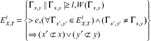
Our similarity measure between two sequences consists of two parts. One is for the conservation part of two sequences, another is for the remains. Our algorithm for similarity of conservation part resembles the SMS algorithm. They differ in the constraint of the matched segment. In SMS algorithm, the key set of matched subsequences Γ_{x, y}, $E_{X,Y}^l$ is defined as follows:

$$E_{X,Y}^l=\left\{\begin{array}{l}{\Gamma }_{x,y}\Vert {\Gamma }_{x,y}|\ge l,\left(\forall {\Gamma }_{x\text{'},y\text{'}}\in E_{X,Y}^l\right)\\ \wedge \left({\Gamma }_{x\text{'},y\text{'}}\ne {\Gamma }_{x,y}\right)\Rightarrow \left(x\text{'}\not\subset x\right)\vee \left(y\text{'}\not\subset y\right)\end{array}\right\}$$

where x and y are two identical subsequences belonging respectively to sequence X and Y, and Γ _{x, y} represents the matched subsequence of x and y. While in our algorithm, the set of matched subsequences is defined as follows:

$$E_{X,Y}^l=\left\{\begin{array}{l}{\Gamma }_{x,y}\Vert {\Gamma }_{x,y}|\ge l,W\left({\Gamma }_{x,y}\right)\\ >e,\left(\forall {\Gamma }_{x\text{'},y\text{'}}\in E_{X,Y}^l\right)\wedge \left({\Gamma }_{x\text{'},y\text{'}}\ne {\Gamma }_{x,y}\right)\\ \Rightarrow \left(x\text{'}\not\subset x\right)\vee \left(y\text{'}\not\subset y\right)\end{array}\right\}$$

where subsequences x and y are not required to be identical but the matching score of x and y, W(Γ _{x, y} ), need to larger than e. The detail algorithm can refer to the paper. ¹

For two divergent sequences, the conservation of subsequences may account for a small part of the entire sequence. In order to calculate accurately the similarity between two protein sequences, we should consider the similarity between the remained sequences which exclude the matched subsequences. Because the divergent sequences, the alignments metric and alignment-free metric have same discriminate power, ²⁴ we use alignment-free metric, standard Euclidean distance, which have advantage of light computational load.

A protein sequence, X, of length n, is a linear succession of n symbols from the alphabet of all possible amino acids. An L-tuple is a segment of L symbols. The set W _L consists of all possible L-tuples that can be extracted from protein sequence X, and has K elements (Equation 1).

$$W_L=\left\{w_{L,1},w_{L,2},\mathrm{...},w_{L,K}\right\},\hspace{1em}K={20}^L$$

(1)

The mapping of X into the Euclidean space can be defined by representing X by its amino acid L-tuple in count, $C_L^X$ :

$$c_L^X=\left(c_{L,1}^X,\mathrm{...},c_{L,K}^X\right)$$

(2)

where $c_{L,i}^X$ is the counting occurrences of w_{L, i} with overlapping in sequence X.

We use the standard Euclidean distance to represent the dissimilarity of remained sequences. Supposed sequences X′ and Y′ are remains excluding the matched subsequences. The standard Euclidean distance is defined by

$$d^{SE}\left(X\text{'},Y\text{'}\right)={\left(c^{X\text{'}}-c^{y\text{'}}\right)}^T\times {\left[diag\left(s_{11},\mathrm{...},s_{KK}\right)\right]}^{-1}\times \left(c^{X\text{'}}-c^{Y\text{'}}\right)$$

(3)

where s₁₁, …, s _KK is the diagonal element of the covariance matrix of L-tuple counts.

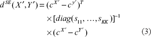
In order to obtain the similarity between sequences X′ and Y′, we will use function

$$f\left(d\right)=e^{-\beta d}$$

(4)

to transform distance measures to similarity measures. The d in Equation (4) denotes the standard Euclidean distance, and the β is a positive, tunable parameter. Accordingly, the similarity of sequences X and Y is defined as follows:

$$S_{X,Y}=S_{X,Y}^M+e^{-\beta d^{SE}\left(x\text{'},Y\text{'}\right)}$$

(5)

where $S_{X,Y}^M$ represents the similarity of the matched subsequence of two sequences.

2.2. Clustering algorithm

Given a set D of N data, the clustering problem can be described as follows:

Partitioning the set D into m subsets, C₁, …, C _m , such that

$$C_i\ne \varnothing ;C_i\cap C_j=\varnothing ,i\ne j;{\cup }_{i=1}^m{C}_i=D;i,j=1,\dots ,m$$

Affinity propagation takes as input a collection of similarities between each pair of data points and outputs a vector c of exemplars, c = [c₁,…,c _N ]. For the data d _i in D, the c _i represent its exemplar. Supposed there are m different values, e₁, …, e _m , in vector c, a partition of D can be described by C _i = {D _j | c _j = e _i , j = 1, …, N}, i = 1, …, m. Initially Affinity propagation views each data as a potential exemplar, and identifies the exemplar by pass massages between data points. There are two kinds of massages and each considers a different kind of competition. The responsibility r(i, k) is sent from data i to the candidate exemplar point k, which implies the reliability of point k served as the exemplar of point i. The availability a(i, k) is sent back from the candidate exemplar point k to point i, which denotes the appropriateness for point i to choose point k as its exemplar. The update rules are described below ¹¹ :

Initialization:

$$r\left(i,k\right)=0,a\left(k,i\right)=0\hspace{1em}foralli,k$$

Responsibility updates:

$$r\left(i,k\right)\leftarrow s\left(i,k\right)-\underset{j:j\ne k}{\max }\left(a\left(j,i\right)+s\left(i,j\right)\right)$$

Availability updates:

$$a\left(k,k\right)\leftarrow \sum _{j:j\ne k}\max \left\{0,r\left(j,k\right)\right\}$$

$$a\left(k,i\right)\leftarrow \min \left(0,r\left(k,k\right)+\sum _{j:j\notin \left\{k,i\right\}}\max \left\{0,r\left(j,k\right)\right\}\right)$$

Making assignments:

$$c_i^{*}\leftarrow \underset{k}{\arg \hspace{0.17em}\max }r\left(i,k\right)+a\left(k,i\right)$$

Here s(i, i) is preference and is inputted by the user. The value of s(i, i) reflects the possibility that point i is chosen as an exemplar. If there is no priori knowledge, the probability for all data points are equal lead to a common preference value. The preference value can be varied to produce different numbers of clusters. In general, small preference value results in a small number of clusters. There is no definite method to choose an optimal preference. Frey and Dueck suggested that the value of preference could be the median or the minimum of the input similarities. But in practical, these values do not give a satisfying clustering.

Postaire et al have proposed an assumption that, when true clusters exist, stable number of clusters appears for a wide range of value of preference. ²⁵ Based on this assumption, the choice procedure can be described bellow: running algorithm using a range of parameter, choosing such a parameter in the middle of the largest range where the number of detected clusters remains constant. This procedure has proved to be a good method to optimize a number of clustering algorithms. ²⁶ Therefore, we also apply this method to determine the preference. We first choose the minimum and maximum of the input similarities as the up bound and down bound of preference range, respectively, and draw uniformly 100 values as preference from the range to run the AP algorithm. We then apply the procedure outlined above to find a appropriate value of preference.

2.3. Clustering validation

To assess the ability of a clustering algorithm to recover true cluster structure it is necessary to define a measure of agreement between two partitions; the first partitions being a priori known clustering structure of the data; and the second partition obtaining from the clustering algorithm. The F-measure ²⁷ described bellow is a measure of agreement between two partitions.

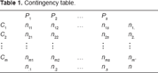
Consider C = {C₁, …, C _m } is a clustering structure given by an algorithm of the test data set X and P = {P₁, …, P _s } is a defined partition of data. We use a contingency table (Table 2) to express the partitional agreement. The entry n _ij denotes the number of proteins that are both in clusters C _i and P _j . Let $n_i={\sum }_{j=1}^m{n}_{ij}$ and $n_{\cdot j}={\sum }_{j=1}^s{n}_{ij}$ denote the row and column sums of the contingency table, respectively. Clearly, n _i. and n _.j are the number of proteins in classes C _i and P _j and $n={\sum }_{i=1}^m{n}_{i.}={\sum }_{j=1}^s{n}_{\cdot j}$ is the number of total proteins.

Table 1.

Contingency table.

	P 1	P 2	…	P s
C 1	n 11	n 12	…	n 1s	n 1.
C 2	n 21	n 222		n 2s	n 2.
⋮	⋮	⋮		⋮	⋮
C m	n m1	n m2	…	n ms	n m .
	n .1	n .2	…	n .s	n

Table 2.

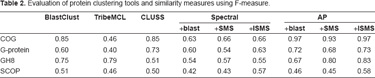
Evaluation of protein clustering tools and similarity measures using F-measure.

	BlastClust	TribeMCL	CLUSS	Spectral			AP
				+blast	+SMS	+ISMS	+blast	+SMS	+ISMS
COG	0.85	0.46	0.85	0.63	0.66	0.66	0.97	0.93	0.97
G-protein	0.60	0.40	0.73	0.60	0.54	0.63	0.72	0.68	0.73
GH8	0.75	0.79	0.51	0.54	0.57	0.55	0.67	0.80	0.83
SCOP	0.51	0.46	0.50	0.42	0.43	0.57	0.46	0.45	0.58

We define the precision of C _i with respect to P _j , Pre(i, j), as the ratio of the number of proteins of P _j assigned to C _i to the number of proteins in C _i. , i.e. Pre(i, j) = n _ij /n _i. ; The recall of C _i with respect to P _j , Rec(i, j), is defined as the ratio of the number of proteins of P _j assigned to C _i to the number of proteins in P _j , i.e. Rec(i, j) = n _ij /n _.j ; The F-measure is then defined as:

$$F\left(C,P\right)=\frac{1}{n}\sum _{j=1}^s{n}_{.j}\underset{i}{\max }\frac{1}{\frac{1}{2}\left(\frac{1}{\text{pr e}\left(i,j\right)}+\frac{1}{\mathrm{Re}\hspace{0.17em}c\left(i,j\right)}\right)}=\frac{1}{n}\sum _{j=1}^s{n}_{.j}\underset{i}{\max }\frac{2n_{ij}}{n_{i.}+n_{.j}}$$

Clearly, an F-measure has a value between 0 and 1. The closer the F-measure to 1, the better agreement two partitions display and an F-measure of 1 indicates identity of two partitions.

2.4. Datasets

Dataset A

The database of Clusters of Orthologous Groups of proteins (COGs) ²⁸ is an attempt on a phylogenetic classification of the proteins, currently consists of 5665 COGS from 192,987 proteins encoded in 66 complete genomes of bacteria, archaea and eukaryotes (http://www.ncbi.nlm.nih.gov/ COG). The proteins in a COG are considered as orthologs, if they come from individual orthologous genes, or orthologous sets of paralogs if they belong to different lineages. Accordingly, Each COG is assumed to have evolved from an ancestral protein. To illustrate the efficiency of clustering algorithms in grouping protein sequences classified by phylogenetic relationships, we draw randomly 412 protein sequences of 7 COGs from the COG database.

Dataset B

G proteins, ²⁹ short for guanine nucleotide-binding proteins, is a family of important signal transducing molecules in cells. G-proteins receive the signal from different receptor; altering an inactive guanosine diphosphate (GDP) bound state to active guanosine triphosphate (GTP) bound state, ultimately active according to effectors to regulate different cell processes. This family has been the subject of a considerable number of publications by researchers around the world, so we considered it a good reference classification to test the performance of clustering algorithms. ¹ The G-proteins datasets consists of 252 protein sequences belonging to 6 classes, include G protein alpha G(12), G protein alpha G(i/o/t/z), G protein alpha G(q), G protein alpha G(s), G protein alpha other.

Dataset C

The CAZy (carbohydrate-active enzymes) ³⁰ database describes the families of structurally-related catalytic and carbohydrate-binding modules (or functional domains) of enzymes that degrade, modify, or create glycosidic bonds. Glycoside Hydrolases are a widespread group of enzymes which hydrolyze the glycosidic bond between two or more carbohydrates or between a carbohydrate and a non-carbohydrate moiety. The proteins belonging to the Glycoside Hydrolases families have multi-domain which are known to be hard to align and have not yet been definitively aligned. To evaluate the performances of clustering algorithms with multi-domain protein families, we select 147 proteins belonging to the Glycoside Hydrolases family 8 as the test databases. In addition, we choose the 33 (α/β)₈ barrel proteins, studied recently by Côté et al ³¹ and Fukamizo et al, ³² as another test dataset. The periodic character of the catalytic module known as “(α/β)₈ barrel” makes these sequences hard-to align using classical alignment approaches. ¹

Dataset D

The SCOP (Structural Classification of Proteins) ³³ is a database of proteins of known structure, among which the structural and evolutionary relationship is comprehensively described. It has been organized in a hierarchy by manual inspection and used by a series of automated methods. The fundamental unit of classification is a domain in which the structure is determined experimentally. Above domain, the hierarchies of SCOP consist of Species, Protein, Family, Superfamily, Fold, Class, in turn. The proteins in a species are natural or artificial variants of a protein. The similar sequences of the same function are grouped into Proteins. A Family includes the proteins with related sequences but typically distinct functions. The structural and functional features of the proteins in same Superfamily suggest that a common evolutional origin is probable. Fold contains the protein with same characteristic features and similar structure, whereas proteins in the same class share the same secondary structures in same arrangement with the same topological connections. Because there are many domains in the SCOP dataset shared a very high degree of similarity, it is frequently helpful to reduce the redundancy for a further task. The ASTRAL ³⁴ compendium addresses this issue by selecting high-quality representative from the SCOP dataset according to different thresholds and measures of sequence similarity. We use the ASTRAL SCOP 1.71 with a threshold of 95%, which means the domain sequences from this set share less than 95% identity to each other, as test data source. The test dataset selected randomly from ASTRAL consists of 590 protein sequences from 5 superfamilies.

3. Results and Discussion

To illustrate the efficiency of our method, we tested AP algorithm with our similarity measure extensively on all the protein datasets above and compared it with several widely used clustering algorithms, CLUSS, BlastClust, TribeMCL, Spectral clustering. In order to display the influence of different similarity measures, we performed tests on all datasets using three measures, which server as the input of Spectral clustering and AP algorithm. These measures include blast, which chose the negative logarithm of BLAST E-values as a similarity measure between two sequences, SMS and our similarity measure ISMS (improved SMS). In order to obtain the best possible performance of TribeMCL, we varied the input parameters, inflation, to evaluate the results on the same data. And the same things were done to BlastClust. Here we present the results of each algorithm obtained on all datasets of experiments in Table 2 and the obtained numbers of clusters in Table 3.

Table 3.

Clustering results of the dataset. Number of clusters obtained by clustering the protein sequences of 4 datasets (rows) with each of the clustering algorithms tested (columns). The last column represent the number of clusters of references sets.

	BlastClust	TribeMCL	CLUSS	Spectral			AP			Dataset
				+blast	+SMS	+ISMS	+blast	+SMS	+ISMS
COG	10	250	7	8	30	20	10	6	8	7
G-protein	69	19	24	15	21	21	9	8	9	6
GH8	39	39	58	3	10	19	5	3	3	11
SCOP	145	252	15	8	30	7	23	13	6	5

From Table 2 and Table 3, we can observe that the AP clustering with ISMS clearly outperforms the other methods. First of all, it detects a number of clusters which is close to the correct number of dataset. For instance, in G-protein dataset, AP+ISMS method detects 9 clusters; at the same time, BlastClust detects 69 clusters, the TribeMCL detects 19 clusters, CLUSS detects 24 clusters and Spectral clustering detects 15 clusters (Spectral + blast). On the other hand, the better quality of the clustering is quantified by the F-measure. For each of the protein dataset, the results in Table 2 show clearly that Affinity propagation obtained the best F-measure. In our experiments, on average, the value of the F-measure given by AP + ISMS is 15% better than BlastClust, 56% better than TribeMCL, 23% better than CLUSS, and 42% better than best results of Spectral clustering.

We also observe that using same similarity measure the AP achieves best cluster quantity. We first analyze the influence of similarity measure on clustering quality. For COG and G-protein datasets, AP algorithm gets almost same F-measure. The reason is that sequences in COG and G-protein datasets share high similarity which leads to similar similarity measures given by three methods. In fact, the strategy of blast to calculate the similarity bears some resemblance to the one of SMS. They also depend on the conserved segments between two sequences. The difference lies in that blast does not take into account the circular permutation and tandem repeats of segments. However, in COG and G-protein datasets, there are not these hard-to-align protein sequences. So blast and SMS tend to obtain similar similarities. As for ISMS, high similarities between sequences result in that the dissimilar parts between two sequences play little role in calculation of similarity. Consequently, three methods obtain the similar similarity measures. These results imply that it is AP algorithm that leads to better clustering quality.

While on GH8 dataset, AP algorithm gains better clustering quality using SMS and ISMS than blast. Because GH8 is a multi-domain protein family, similarity measures based on alignment, for instance, blast, cannot describe accurately similarity between sequences in this family. For sequences in SCOP dataset, which share low sequence similarity, ISMS which take into account homogeneous segment pairs and dissimilarity parts, will describe the similarity better than blast and SMS do. For datasets from SCOP, BlastClust and TribeMCL tend to create more clusters than reference clusters. We will analyze the reason from the algorithm point of view.

In BlastClust, two sequences are considered to be neighbored if their similarity is above a certain threshold. If a sequence is a neighbor to at least one sequence in a cluster, this sequence will be put into this cluster. Too many clusters achieved by BlastClust mean that the similarities of many sequences were not detected by blast. On the other hand, TribeMCL is based on random walks on the similarity graph, where a vertex represents a sequence and an edge connecting two vertices is weighted by the similarity between these two vertices. A random walk on a graph is a stochastic process which randomly jumps from vertex to vertex. The idea of the TribleMCL algorithm is that, if the random walks can somehow be biased, say by pruning weak edges (low weight) and reinforcing strong edges (high weight) simultaneously, clusters may emerge from the graph. Formally, the transition probability of jumping in one step from vertex i to vertex j is proportional to the edge weight w _ij . Creating too many clusters means that, for the sake of similarities, random walks can not jumps from some vertices to other vertices which are in same reference cluster. Therefore, from the results of BlastClust and TribeMCL, we can imply that Blast is not capable to detect the similarities between sequences in the SCOP. SMS also can not effectively describe the similarities between sequences in the SCOP, which can be confirmed by the fact that Spectral clustering and AP achieve almost same F-measure when using Blast and SMS measure, respectively. However we obtain an improvement of F-measure when Spectral clustering and AP apply ISMS to measure the sequence similarities. These results provide good evidences supporting our points that ISMS can measure similarities more accurately than Blast and SMS do on condition that sequence similarities is low.

The experimental results for 33 (α/β)₈ barrel proteins with the different algorithms are summarized in Table 4, which shows the cluster correspondence of each of the sequences by algorithm used. The 33 (α/β)₈ barrel proteins are subdivided by Affinity propagation with ISMS as the input into five subfamilies, corresponding to their known biochemical activities. Further, in contrast with other algorithms, Affinity propagation algorithm with ISMS classified all the 33 (α/β)₈ barrel proteins in the same subfamilies obtained by Côté, et al. The first cluster includes enzymes with “β-mannosidase” activities; the second cluster includes enzymes with “β-mannosidase” activities; the third cluster includes enzymes with “β-glucuronidase” activities; the forth cluster includes enzymes with “β-galactosidase” activities; the fifth cluster includes enzymes with “exo-β-D-glucosaminidase” activities. While the other algorithms do not succeed to obtain clustering results that correspond to the functional classification of 33 (α/β)₈ barrel proteins. Since, CLUSS has classified the two proteins MaC and MaT with wrong cluster. As for BlastClust and TribeMCL, there are a number of proteins which could not be classified by BlastClust, and a number of proteins which were wrongly classified by TribeMCL. These results show the superiority of our method over other algorithms. When we take the similarity matrices obtained by our method ISMS as the input of Spectral clustering (8th column, Table 4), this algorithm can also group proteins into correct cluster. In addition, there are also a few proteins are classified to wrong cluster when using Spectral clustering and AP algorithm with blast and SMS similarity as input. These results show that our method can estimate the similarity between two proteins more accurately than other methods do. That is to say, ISMS more accurately highlights the characteristics of the biochemical activities and modular structures of the clustered protein sequences than do other similarity measure.

Table 4.

Clustering results of the 33 (α/β)₈ barrel protein. Each of rows represent a 33 (α/β)₈ barrel protein. The corresponding cluster obtained by Côté et al. and Fukamizo et al. is represented in the first column of the table as reference. The other columns correspond to the clustering results of tested algorithms. Each number in the table represents the corresponding cluster of the row's protein sequence obtained with the column's method. They are italic when they don't correspond to reference classification. The symbol “/” means that the row's protein sequence is unclustered.

Protein sequences	Côté Fukamizo	CLUSS	BlastClust	TribeMCL	Spectral			AP
					+blast	+SMS	+ISMS	+blast	+SMS	+ISMS
GaEco	1	1	1	1	1	1	1	1	1	1
GaA	1	1	/	1	1	1	1	1	1	1
GaK	1	1	/	1	1	1	1	1	1	1
GaC	1	1	/	1	1	1	1	1	1	1
GaEcl	1	1	1	1	1	1	1	1	1	1
GaL	1	1	1	1	1	1	1	1	1	1
MaA	2	2	2	1	2	/	2	2	2	2
MaB	2	2	2	2	2	2	2	2	2	2
MaH	2	2	2	2	2	2	2	2	2	2
MaM	2	2	2	2	2	2	2	2	2	2
MaC	2	3	2	1	2	/	2	2	3	2
MaT	2	3	2	1	2	/	2	4	3	2
UnA	3	3	3	2	2	3	3	2	3	3
UnBv	3	3	3	2	2	3	3	2	3	3
UnBc	3	3	/	2	2	3	3	2	3	3
UnBm	3	3	3	2	2	/	3	2	3	3
UnBp	3	3	3	2	2	/	3	2	3	3
UnR	3	3	3	2	2	3	3	2	3	3
CsAo	4	4	/	1	2	/	4	2	4	4
CsS	4	4	4	1	2	/	4	4	4	4
CsG	4	4	4	1	2	4	4	4	4	4
CsM	4	4	4	1	2	4	4	4	4	4
CsN	4	4	/	1	2	4	4	4	4	4
CsAn	4	4	/	1	2	4	4	4	4	4
CsH	4	4	4	1	2	4	4	4	4	4
CsE	4	4	4	1	2	4	4	4	4	4
GIC	5	5	5	1	1	5	5	5	5	5
GIE	5	5	5	1	1	5	5	5	5	5
GIH	5	5	5	1	1	5	5	5	5	5
GIL	5	5	5	1	1	5	5	5	5	5
GIM	5	5	5	1	1	5	5	5	5	5
GIF	5	5	5	1	1	5	5	5	5	5
GIS	5	5	5	1	1	5	5	5	5	5

4. Conclusions

Clustering of protein sequences into correct evolutionary related protein groups using only sequence information is a difficult problem. In this paper, we have proposed an improved similarity measure ISMS based on which we group the protein sequences using Affinity propagation algorithm. We have compared the results obtained by AP algorithm with those obtained by BlastClust, TribeMCL, CLUSS and Spectral clustering on extensive datasets. The AP algorithm used jointly with ISMS yields an improved performance over the other methods in terms of the quality of the clusters as measured by the F-measure. Moreover, the number of clusters returned by the AP algorithm with ISMS is in general much closer to the correct one than the one returned by the other methods. Moreover, using the similarities estimated by ISMS on 33 (α/β) 8-barrel proteins dataset, Spectral clustering and AP all retain the correct clusters. This means that our improved similarity measure reflects biologically correlation between two sequences than the other measures do.

Disclosure

The authors report no conflicts of interest.