Top-Down Clustering for Protein Subfamily Identification

Abstract

We propose a novel method for the task of protein subfamily identification; that is, finding subgroups of functionally closely related sequences within a protein family. In line with phylogenomic analysis, the method first builds a hierarchical tree using as input a multiple alignment of the protein sequences, then uses a post-pruning procedure to extract clusters from the tree. Differently from existing methods, it constructs the hierarchical tree top-down, rather than bottom-up and associates particular mutations with each division into subclusters. The motivating hypothesis for this method is that it may yield a better tree topology with more accurate subfamily identification as a result and additionally indicates functionally important sites and allows for easy classification of new proteins. A thorough experimental evaluation confirms the hypothesis. The novel method yields more accurate clusters and a better tree topology than the state-of-the-art method SCI-PHY, identifies known functional sites, and identifies mutations that alone allow for classifying new sequences with an accuracy approaching that of hidden Markov models.

Introduction

We consider the task of protein subfamily identification: given a set of sequences that belong to one protein family, the goal is to identify subsets of functionally closely related sequences (called subfamilies). This is in essence a clustering task. Most current methods for subfamily identification use a bottom-up clustering method to construct a cluster hierarchy, then cut the hierarchy at the most appropriate locations to obtain a single partitioning. Such approaches rely on the assumption that functionally similar proteins have sequences with a high overall similarity but do not exploit the fact that these sequences are likely to be highly conserved at particular positions. This raises the question to what extent clustering procedures can be improved by making them exploit this property.

In this article, we propose and evaluate an alternative clustering procedure that does exactly this. The procedure uses the “top-down induction of clustering trees” approach proposed by Blockeel et al. ¹ This approach differs from bottom-up clustering methods in that it forms clusters whose elements do not only have high overall similarity but also have particular properties in common. In the case of subfamily identification, these properties can be the amino acids found at particular positions.

Apart from possibly yielding higher quality clusterings, this approach has the advantage that it automatically identifies functionally important positions and that new sequences can be classified into subfamilies by just checking those positions.

We evaluate the proposed approach on eleven publicly available datasets using a wide range of evaluation measures. We evaluate the predicted clustering as well as the underlying tree topology for which we propose two new measures. Our results show that splits based on polymorphic positions (ie, positions that have more than one amino acid residue) are highly discriminative between protein subfamilies, that using such splits to guide a clustering procedure improves protein subfamily identification, that the identified positions yield accurate classification of new sequences, and that the resulting clustering tree identifies functionally important sites.

Methods

We first describe our novel method for protein subfamily identification. Next, we briefly describe SCI-PHY, the state-of-the-art approach that we use as a reference point. Finally, we review the evaluation measures used in this paper.

Proposed method

Sequences within a protein subfamily are not only similar to each other, they are also characterized by a small set of conserved amino acids at particular locations, which distinguish them from sequences in other subfamilies. The method we propose exploits this property. It creates clusters in which sequences are not only globally similar, but additionally, identical in particular locations. These locations are discovered by the clustering process as it goes.

The method works top-down. It starts with a set of sequences, which is given as a multiple sequence alignment, and tries to split it into subsets such that (1) sequences within a subset are similar and (2) the split is defined by a test of the form p = a, or more generally p ∈ S, with p a location, a an amino acid, and S a set of amino acids.

Figure 1 illustrates the effect of only allowing splits that can be defined by tests based on polymorphic positions. It shows how a set of sequences (S1 to S5) is split into two clusters, (S1, S3, S5) and (S2, S4), based on the test p6 = R that returns true for one cluster and false for the other. Looking only at overall sequence similarity, the clusters (S1, S3, S4, S5) and (S2) would be equally good, but from the biological point of view, the clustering with preserved amino acids within subclusters is preferred.

Figure 1.

Illustration of a split based on a polymorphic position.

After dividing a set into two subsets, the same principle can be used to further subdivide the subsets up to the level of singletons (subsets with only one sequence). This yields a hierarchical tree. For the purpose of subfamily identification, the tree is cut at particular locations, and the resulting clusters are assumed to form subfamilies.

Our method is implemented on top of Clus (http://dtai.cs.kuleuvenbe/clus/), a general-purpose system for top-down clustering ¹ that follows exactly this procedure. Pseudocode is shown in Figure 2. In a first phase (GrowTree), the method starts with splitting the whole dataset then recursively splits subsets up to the level of single sequences. To split a set, the algorithm tries all possible tests of the form p ∈ S with p, a location, and S, a set of amino acids^a. It tentatively splits the set according to each test, evaluates this split (according to a certain heuristic), and remembers the best one. It finally splits the set according to the best test encountered. In a second phase (PruneTree), the tree is pruned. In a single pruning step, a pair of sibling leaves is pruned, turning their parent into a leaf. Which pair is pruned is determined by a pruning heuristic. This step is continued until the whole tree is reduced to a single node. Each tree encountered in the process defines a clustering, the leaves of the tree being the clusters. Among all the trees thus found, the one with the highest-quality clustering is returned as the final result.

Figure 2.

Pseudocode for the Clus-based approach.

The resulting clusters, which correspond to the predicted protein subfamilies, are then output along with the underlying tree, which explicates how the clusters were split and which tests were used. We show an example of such a tree in Figure 3. Note that the internal nodes typically contain multiple tests. This indicates that there are equivalent tests for that stage of the clustering process; tests are equivalent when they yield the same outcome for all the sequences.

Figure 3.

Example of a tree output by our method.

Apart from identifying subfamilies, the tree has two additional advantages. First, it allows for easy classification of new sequences into a subfamily. Starting at the root node, a new sequence is moved down the tree according to the outcome of the tests until it is classified into one of the predicted subfamilies. When not all tests in a node agree (which is impossible for the sequences used to build the tree, but may happen for other sequences), the majority decides. Second, the identified tests result in a candidate list of functionally important sites, that is, positions that are likely to play a role in the subfamily-specific functions. Protein functional site prediction is an important step in the functional analysis of new proteins (eg, Bickel et al, ² Cheng et al, ³ and Bray et al ⁴ ). As biological validation is costly, providing a first selection of potential sites is an important advantage of our method.

Important parameters of the method are the heuristics used during tree growing (to select the best test to split the data at each step) and pruning (to evaluate the quality of a tree). We now discuss these in detail. We will end this section with a note on the computational complexity of the method.

Test selection heuristics

In the experimental section, we explore three test selection heuristics. Two of them are standard for hierarchical tree learners: maximization of the average intercluster distance and maximization of the minimum intercluster distance. We call the versions of Clus that use these heuristics Clus-MaxAvgDist and Clus-MaxMinDist, respectively.

These heuristics do not take into account the particular requirements of the phylogenetic context. Using the average distance heuristic, for example, one essentially gets the top-down counterpart of the UPGMA algorithm, ⁵ which is known to have some undesirable behavior. ⁶ Therefore, we include a third heuristic, which was designed specifically for the phylogenetic context. ⁷ This heuristic is based on the principle of minimum evolution and it can be seen as the top-down counterpart of the criterion used by the well-know phylogenetic method Neighbor Joining. ⁸ More specifically, it estimates the total branch length of the final tree that will be obtained if a particular test is chosen at this point and prefers the test that minimizes this estimate. We call the version of Clus with this heuristic Clus-MinLength. For the exact formula and more details about this heuristic, see Vens et al. ⁷

The proposed selection heuristics make use of distances between pairs of amino acid sequences. Our method computes distances based on the Jones-Taylor-Thornton matrix, ⁹ which is a model of amino acid substitution widely used for phylogenetic inference. Alternatively, we allow the user to give a pairwise distance matrix as input.

Extracting clusters from the hierarchical tree

The quality measure used during pruning is encoding cost,^10,11 which can be interpreted as the cost to encode a clustering given the homogeneity of the clusters and the number of clusters. Ideally, one wants to achieve two goals: to have as few clusters as possible and to have maximally homogeneous clusters. There is a trade-off between these two goals, as having fewer clusters implies larger clusters, which are less likely to be homogeneous. The encoding cost (Equation 1) combines these two goals.

$$Encoding\hspace{0.17em}cost=Nlogk-{\sum }_{l=1}^k{\sum }_i\log \mathrm{Pr}\left({\text{n}}_{\text{li}}|\alpha \right)$$

(1)

The first component of the equation is the cost associated to the number of subfamilies, the second component is the cost to encode each subtree alignment for a certain clustering. More specifically, N is the number of sequences, k is the number of clusters, and Pr(n_li | α) is the probability of n_li, which is the count vector of observed amino acids for subfamily l at column i, under a Dirichlet mixture density α. Dirichlet mixture densities ¹² contain prior information about amino acids and, when combined with observed amino acid frequencies, provide estimates of expected amino acid probabilities. ¹⁰

Computational complexity

The computational complexity of the proposed method is O(aN ² logN), with a the alignment length and N the number of sequences. We obtain this complexity by adding the complexity of the tree building and postpruning procedures, as described next.

The complexity to construct the tree is O(aN ² logN) under the assumption that a reasonably symmetric tree is built (the depth of which is logarithmic in the number of leaves). ⁷ In order to extract subfamilies from the tree, every pruning step and every merging candidate requires calculating Equation 1. In two subsequent calculations, most of the clusters remain the same, and therefore most of the Σ _i log Pr(n_li | a) terms do not change. We can avoid recomputing these values by calculating them only once for every node (cluster) and storing them. As a (complete) tree with N sequences contains 2N − 1 nodes, and the computation of Equation 1 has a complexity O(aN), the resulting complexity of the cluster extraction is O(aN ² ), leading to an overall complexity of O(aN ² logN) for the complete method.

SCI-PHY

To identify protein subfamilies, SCI-PHY ¹¹ first builds a hierarchical tree bottom-up. It then extracts clusters from the tree, which are output as the predicted subfamilies.

The tree construction process starts with each sequence being a separate cluster. Then, for each cluster, a profile is defined, which gives the expected amino acid probabilities for each position based on the observed amino acid distribution and a Dirichlet mixture density. ¹² Next, using relative entropy ¹³ to estimate the distance between the profiles, the two closest profiles are merged, and a profile for the new cluster is created. This merging procedure is repeated until all sequences are part of the same cluster. Finally, the resulting tree topology is given as input to a postpruning procedure. This pruning procedure returns the stage in the clustering procedure with minimal encoding cost.

Once the protein subfamilies have been predicted, SCI-PHY can classify new protein sequences into one of these subfamilies by subfamily hidden Markov model (SHMM) construction. ¹⁴ A SHMM is built for each subfamily, and the best match with the query sequence is predicted.

We use SCI-PHY in our experimental comparison (Results and Discussion) because it has been extensively evaluated: it was compared to several methods, and was shown to give comparable or superior results.^11,15 To our knowledge, no other method has been shown to give better results.

Evaluation measure

In the Results and Discussion section, we evaluate the subfamilies output by Clus and SCI-PHY on a number of datasets for which the true subfamilies (reference clustering) are known. We evaluate both the tree topology from which clusters are extracted and the clusters themselves. The reason for evaluating also the tree topology is three-fold. First, as the authors of SCI-PHY also point out, the definition of the “right” clusters is somewhat arbitrary, since subfamilies can be defined on several levels of granularity. By evaluating the tree topology, which defines clusterings on multiple levels, we can analyze how the reference clustering is represented in the tree. Second, we can evaluate the results regardless of the quality of the pruning procedure. Third, the tree is often interesting in itself, as it can help biologists to interpret the predicted clustering and obtain insights in how the clusters are related.

Tree topology evaluation

We evaluate tree topologies using three measures: tree-based classification error, ¹⁶ edited tree size, and number of subfamily changes.

Edited tree size

The edited tree size indicates how compact the smallest possible pure clustering derived from the tree is. It is calculated by repeatedly merging sibling leaves that belong to the same subfamily until such merging is no longer possible.

Consider the two trees shown in Figure 4, for example. They have five sequences, three of which belong to subfamily 1 (S1), and two of which belong to subfamily 2 (S2). The edited tree for tree a would merge the S2 sequences, resulting in an edited tree size of 4. The edited tree for tree b would merge the two S1 sequences connected by branches r₇ and r₈, also resulting in an edited tree size of 4.

Figure 4.

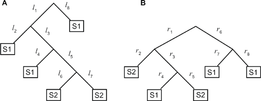
Two trees with the same edited tree size, a smaller TBC error for tree a, and a smaller number of subfamily changes for tree b.

Tree-based classification error

Similarly to the edited tree size, the tree-based classification (TBC) error ¹⁶ evaluates to which extent the tree places sequences from the same subfamily in the same subtree. While the former considers clusters that are pure and as large as possible, the TBC error considers clusters that minimize the number of “classification errors” in the derived clustering, as follows.

A subtree is said to be “good” for a subfamily F if more than half of its sequences belong to F and more than half of F's sequences belong to the subtree. Given a set of disjoint good subtrees, a sequence is considered correctly classified if it occurs in a good subtree for its subfamily, and incorrectly classified otherwise. The TBC error is defined as the smallest number of incorrectly classified sequences in any set of disjoint good subtrees.

Tree a in Figure 4 defines two good subtrees: a cut in branch l₅ yields a good subtree for S2 (with three classification errors), and the complete tree is a good subtree for S1 (with two classification errors). Hence, the TBC error for this tree is two. Tree b defines 3 good subtrees. A cut in r₁ (or r₆) yields two disjoint good subtrees (resulting in 1 classification error): a good subtree for S2 at the left and a good subtree for S1 at the right. The complete tree is again a good subtree for S1, with two classification errors. Hence, the TBC error for this tree is 1. Lazareva-Ulitsky et al ¹⁶ provide a algorithm to compute the TBC error.

The subtrees defined by the TBC error are more permissive than the ones defined by the edited tree size in the sense that clusters are not required to be pure; on the other hand, TBC error is stricter in the case where sequences from the same subfamily are spread over two or more subtrees.

Both measures are dependent on the place of the tree root. If the root of tree A would be in branch l₅, for example, the edited tree size would be 2 instead of 4 and the TBC error would be 0 instead of 2. Although evaluating the rooted tree is important, since the root influences the possible ways in which the tree can be cut, we also propose a measure that is independent of the place of the root.

Number of subfamily changes

If we associate a subfamily (or alternatively, a molecular function) to each internal node of the tree, then we say that a subfamily change occurs for each branch connecting two nodes with different associated subfamilies. For instance, if we associate subfamily 1 to the root of tree a in Figure 4, there is one change to subfamily 2 in branch l₅. The right tree, however, requires 2 subfamily changes (branches r₂ and r₅).

Counting the minimal number of subfamily changes corresponds to counting mutations in parsimony analysis, ¹⁷ where one prefers the phylogenetic tree that requires the least evolutionary change to explain some observed data. Although we consider clustering trees rather than phylogenetic trees, we can directly apply the Fitch parsimony algorithm ¹⁷ to count the number of subfamily changes.

Note that in contrast to the previous two measures, this measure does not penalize a tree for having a ladder-like shape. That is why tree a has a smaller number of subfamily changes, while having the same edited tree size and a higher TBC error as tree b (For an example with larger trees, consider Figures S1 and S2 in the supplemental material. The tree in Figure S1 has an edited tree size of 12, a TBC error of 11, and nine subfamily changes, while the tree in Figure S2 has an edited tree size of 28, a TBC error of 64, and 11 subfamily changes. The larger difference between the trees in their edited tree size and TBC error is due to the ladder-like shape of the tree in Figure S2.). However, it is important to note that the shape of the tree does influence the possible ways to cut it. Therefore, we use the three measures, as they provide complementary information to one another.

Clustering evaluation

We evaluate clusters using three measures earlier used for SCI-PHY ¹¹ (purity, VI distance, and edit distance) and two additional ones: the percentage of sequences in pure clusters and category utility. The first four measures compare the predicted clustering to the reference clustering, while the latter evaluates the quality of the predicted clustering itself, regardless of a given reference clustering.

Purity

Purity is defined as the fraction of clusters in a given clustering that contain instances of only one reference cluster. It assesses the ability of the method to cluster instances of different kinds in different clusters. However, as it does not penalize if instances of one kind are spread over many pure clusters, perfect purity can be achieved when every instance corresponds to a single cluster. Therefore, singletons are not included in the calculation.

Percentage of examples in pure clusters

To complement the information given by purity, we also report the percentage of examples in pure clusters (denoted further as PctExPureC). Again, singleton clusters are discarded.

Edit distance

The edit distance between two clusterings is the number of merge and/or split operations required to transform one clustering into the other one. For example, if instances of three kinds–-A, B, and C–-are clustered in only one cluster, we need two-split operations to separate the three groups of instances. The higher the edit distance is, the more different the clusterings are.

The formal definition of edit distance is given by Equation 2, ¹¹ where Edit (C ¹ ,C ² ) is the edit distance to transform clustering C ¹ into clustering C ² (or the other way around), k' is the number of clusters in C ¹ , k” is the number of clusters in C ² and $r\left(C_m^1,C_n^2\right)$ is equal to 1 if clusters $C_m^1$ and $C_n^2$ have items in common and equal to 0 otherwise.

$$Edit\left(C^1,C^2\right)=2*\left({\sum }_{m=1}^{k^{\prime }}{\sum }_{n=1}^{k^{″}}\left(C_m^1,C_n^2\right)\right)-k^{\prime }-k^{″}$$

(2)

Edit distance penalizes more strongly clusterings for which clusters are too small. For this reason, this measure can be used to counter-balance purity.

VI distance

The VI distance (variation of information distance) measures the amount of information that is not shared between two clusterings. The formula to calculate the VI distance is given by Equation 3, ¹¹ where H(C ¹ ) (Equation 4) is the entropy of clustering C ¹ , and I(C ¹ , C ² ) (Equation 5) is the mutual information between clusterings C ¹ and C ² . In Equation 4, |C_l| is the number of instances in cluster C_l, |C| is the total number of instances in the clustering, and k is the number of clusters in C.

$$VI\left(C^1,C^2\right)=H\left(C^1\right)+H\left(C^2\right)-2*I\left(C^1,C^2\right)$$

(3)

$$H\left(C\right)={\sum }_{l=1}^k\frac{\left|C_l\right|}{C}\log \frac{\left|C_l\right|}{C}$$

(4)

$$I\left(C^1,C^2\right)={\sum }_{m=1}^{k^{\prime }}{\sum }_{n=1}^{k^{″}}\frac{\left|C_m^1\cap C_n^2\right|}{\left|C\right|}log\frac{\left|C_m^1\cap C_n^2\right|}{\left|C\right|}$$

(5)

In Equation 5, $\left|C_m^1\cap C_n^2\right|$ is the number of overlapping instances between clusters $C_m^1$ and $C_n^2$ , k′ and k″ are the number of clusters in C ¹ and C ² , respectively.

Category utility

Category utility ¹⁸ computes the improvement of the predictability of attributes given the clustering in comparison with the situation in which no clustering is defined; in the context of protein subfamily identification, the attributes are the positions in the sequence alignment. The definition of category utility is given by Equation 6, where Pred(A|C) (Equation 7) measures the predictability of the descriptive attributes A giving the clustering C, Pred(A) (Equation 8) measures the predictability of A when no clustering is defined and k is the number of clusters. Note that the division by the number of clusters is important to have a trade-off between improvement of the predictability of attributes and the number of clusters.

$$CU\left(C\right)=\frac{pred\left(A|C\right)-pred\left(A\right)}{k}$$

(6)

$$Pred\left(A|C\right)={\sum }_{l=1}^k\mathrm{Pr}\left(C_l\right){\sum }_i{\sum }_j\mathrm{Pr}{\left(A_i=a_{ij}|C_l\right)}^2$$

(7)

$$Pred(A)={\displaystyle \sum }_i{\displaystyle \sum }_j{(A_i=A_{ij})}^2$$

(8)

In Equation 7, Pr(C_l) is the probability of an arbitrary instance to belong to cluster C_l, i ranges over the instance attributes, j ranges over the possible values for each attribute A, Pr(A_i = a_ij|C₁) is the probability that attribute A_i has value a_ij, given that the instance belongs to cluster C₁. In Equation 8, Pr(A_i = a_ij) is the probability that A_i has value a_ij when no clustering is defined.

Results and Discussion

We empirically evaluate, first, the soundness of the assumptions underlying our method and second, the method's capacity to respectively propose a meaningful tree topology, identify subfamilies, classify new sequences, and identify functional regions. Finally, we discuss related work.

Datasets

We use two groups of datasets. The first group consists of the five EXPERT datasets used by Brown et al ¹¹ to evaluate SCI-PHY. The second group consists of six datasets extracted from NucleaRDB, ¹⁹ which contains protein data for nuclear hormone receptor (NHR) families. These eleven datasets were chosen because for each of them a reliable subfamily identification is provided for every sequence, which gives us a gold standard to evaluate the results.

Each dataset consists of the multiple sequence alignment (MSA) for one protein family. The EXPERT datasets contain sequences from the families Enolase, Crotonase, Secretin, Aminergic (Amine), and NHR. The NucleaRDB datasets contain sequences from the families thyroid hormone like (Thyroid), estrogen like (Estrogen), nerve growth factor IB-like (Nerve), HNF4-like (HNF4), fushi tarazu-F1 like (Fushi), and DAX like (DAX). To construct the NucleaRDB datasets, we used MSAs for each family as provided by NucleaRDB, with replicate sequences removed.

For Amine, NHR, Thyroid, Estrogen, and HNF4, subfamilies are provided at more than one level of granularity. Thus, two sequences can be associated to the same subfamily x in one dataset but to different subfamilies x.1 and x.2 in the other dataset.

Some of the datasets are very unbalanced, complicating the subfamily identification task. For instance, Enolase contains a subfamily consisting of 60% of the sequences. The number of sequences in the subfamilies Crotonase and NHR1 ranges from 1 to 212 (58% of the total 365 sequences) and 139 (34% of the total 412 sequences), respectively.

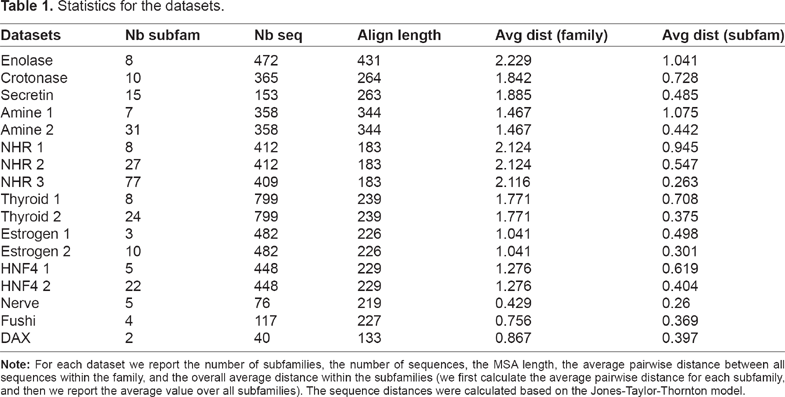
Table 1 shows statistics for the EXPERT and NucleaRDB datasets.

Table 1.

Statistics for the datasets.

Datasets	Nb subfam	Nb seq	Align length	Avg dist (family)	Avg dist (subfam)
Enolase	8	472	431	2.229	1.041
Crotonase	10	365	264	1.842	0.728
Secretin	15	153	263	1.885	0.485
Amine 1	7	358	344	1.467	1.075
Amine 2	31	358	344	1.467	0.442
NHR 1	8	412	183	2.124	0.945
NHR 2	27	412	183	2.124	0.547
NHR 3	77	409	183	2.116	0.263
Thyroid 1	8	799	239	1.771	0.708
Thyroid 2	24	799	239	1.771	0.375
Estrogen 1	3	482	226	1.041	0.498
Estrogen 2	10	482	226	1.041	0.301
HNF4 1	5	448	229	1.276	0.619
HNF4 2	22	448	229	1.276	0.404
Nerve	5	76	219	0.429	0.26
Fushi	4	117	227	0.756	0.369
DAX	2	40	133	0.867	0.397

Note: For each dataset we report the number of subfamilies, the number of sequences, the MSA length, the average pairwise distance between all sequences within the family, and the overall average distance within the subfamilies (we first calculate the average pairwise distance for each subfamily, and then we report the average value over all subfamilies). The sequence distances were calculated based on the Jones-Taylor-Thornton model.

Testing the usability of polymorphic positions for clustering protein subfamilies

In this experiment, we verify our assumption that splits based on polymorphic positions can indeed discriminate protein subfamilies. To that aim, we add the subfamily information to the data and build a classification tree using Clus (ie, we performed supervised learning), without pruning, that is, up to the point where all leaves are pure. Table 2 shows the number of leaves in the resulting tree for each dataset.

Table 2.

Number of leaves in the classification trees (CTs).

Datasets	Nb leaves	Datasets	Nb leaves
Enolase	8	Thyroid 1	13
Crotonase	11	Thyroid 2	38
Secretin	15	Estrogen 1	4
Amine 1	14	Estrogen 2	15
Amine 2	34	HNF4 1	7
NHR 1	11	HNF4 2	36
NHR 2	30	Nerve	5
NHR 3	79	Fushi	4
		DAX	2

Note: The CTs were built using supervised learning. All the leaf nodes in the CTs are pure.

The results show that subfamilies can be perfectly separated from one another using compact trees containing slightly more leaves than the number of subfamilies in the datasets. For five of the datasets, Enolase, Secretin, Nerve, Fushi, and DAX, the classification tree has the same number of leaves as the number of subfamilies. From this we conclude that polymorphic positions are indeed highly discriminant for protein subfamily identification.

The fact that a good clustering tree exists does not imply it will be found by our learner. The above trees are built with the subfamily information, but in a real situation, this will not be the case. In the next sections we evaluate our unsupervised learning method.

Evaluating the tree topology

A first experimental comparison between the three variants of our method (Clus-MinLength, Clus-MaxAvgDist, and Clus-MaxMinDist) on the EXPERT datasets showed better performance for Clus-MinLength, the version adapted to phylogenetic data, than for the other versions, and this for all criteria (see Tables 3, 4, and 5). For this reason, we focus on Clus-MinLength for the remainder of the paper.

Table 3.

Edited tree size: choosing the test selection criterion.

Datasets	clus-MinLength	clus-MaxAvgDist	clus-MaxMinDist
Enolase	12	51	25
Crotonase	33	111	25
Secretin	19	32	21
Amine 1	30	54	33
Amine 2	49	75	48
NHR 1	22	49	36
NHR 2	43	68	41
NHR 3	90	139	107

Note: We indicate the best results in boldface.

Table 4.

TBC error: choosing the test selection criterion.

Datasets	clus-MinLength	clus-MaxAvgDist	clus-MaxMinDist
Enolase	11	90	64
Crotonase	41	99	27
Secretin	8	30	11
Amine 1	178	161	217
Amine 2	41	80	56
NHR 1	36	105	257
NHR 2	24	80	38
NHR 3	42	108	70

Note: We indicate the best results in boldface.

Table 5.

Number of subfamily changes: choosing the test selection criterion.

Datasets	clus-MinLength	clus-MaxAvgDist	clus-MaxMinDist
Enolase	9	14	9
Crotonase	11	37	9
Secretin	15	15	14
Amine 1	16	26	19
Amine 2	37	49	38
NHR 1	10	24	16
NHR 2	29	48	32
NHR 3	78	97	83

Note: We indicate the best results in boldface.

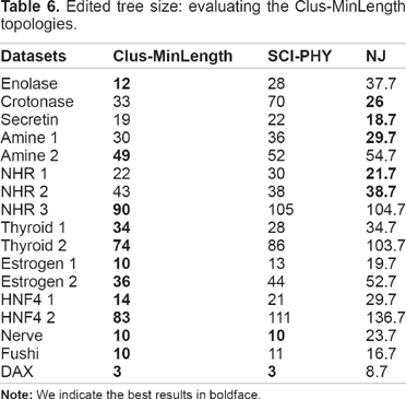
We now evaluate the tree topologies produced by Clus-MinLength in comparison with SCI-PHY for all datasets. For the sake of completeness, we include the phylogenetic tree produced by the Neighbor Joining (NJ) algorithm ⁸ in the comparison. To report the edited tree size and TBC error for NJ, we have to define a tree root since NJ trees are unrooted. The most direct way to do that is to root the tree according to the order in which the sequences were merged by the NJ algorithm. As NJ merges three subtrees in its last step, we root the tree according to each of these subtrees and report the average results. Tables 6, 7, and 8 show the edited tree size, the TBC error, and the number of protein subfamily changes, respectively. For illustration, the (edited) tree topologies for dataset Enolase for the three algorithms are shown in Figures S1 to S3 in the supplemental material.

Table 6.

Edited tree size: evaluating the Clus-MinLength topologies.

Datasets	Clus-MinLength	SCI-PHY	NJ
Enolase	12	28	37.7
Crotonase	33	70	26
Secretin	19	22	18.7
Amine 1	30	36	29.7
Amine 2	49	52	54.7
NHR 1	22	30	21.7
NHR 2	43	38	38.7
NHR 3	90	105	104.7
Thyroid 1	34	28	34.7
Thyroid 2	74	86	103.7
Estrogen 1	10	13	19.7
Estrogen 2	36	44	52.7
HNF4 1	14	21	29.7
HNF4 2	83	111	136.7
Nerve	10	10	23.7
Fushi	10	11	16.7
DAX	3	3	8.7

Note: We indicate the best results in boldface.

Table 7.

TBC error: evaluating the Clus-MinLength topologies.

Datasets	Clus-MinLength	SCI-PHY	NJ
Enolase	11	64	189
Crotonase	41	50	137.3
Secretin	8	13	12.3
Amine 1	178	242	164
Amine 2	41	96	59
NHR 1	36	269	133
NHR 2	24	34	85
NHR 3	42	58	79
Thyroid 1	17	117	55
Thyroid 2	54	130	116
Estrogen 1	2	12	234
Estrogen 2	27	44	161
HNF4 1	4	67	152
HNF4 2	89	202	161
Nerve	11	11	28
Fushi	24	29	53
DAX	3	4	7

Note: We indicate the best results in boldface.

Table 8.

Number of subfamily changes: evaluating the Clus-MinLength topologies.

Datasets	Clus-MinLength	SCI-PHY	NJ
Enolase	9	11	8
Crotonase	11	16	9
Secretin	15	15	14
Amine 1	16	22	12
Amine 2	37	42	35
NHR 1	10	12	7
NHR 2	29	29	26
NHR 3	78	82	77
Thyroid 1	16	17	9
Thyroid 2	39	58	42
Estrogen 1	4	6	5
Estrogen 2	19	27	20
HNF4 1	6	11	6
HNF4 2	50	67	51
Nerve	5	5	5
Fushi	5	6	6
DAX	1	1	1

Note: We indicate the best results in boldface.

Throughout the paper, we report the results of pairwise comparisons as wins/ties/losses. The notation P < 0.05 indicates significance at 5% according to a two-tailed sign test.

In terms of edited tree size (Table 6), Clus-MinLength obtains 13/2/2 (P < 0.05) wins/ties/losses in comparison to SCI-PHY, and 12/0/5 wins/ties/losses in comparison to NJ. The edited tree size for Clus-MinLength, SCI-PHY, and NJ is, on average, 2.6, 3.3, and 3.9 larger than the number of subfamilies.

Table 7 shows that Clus-MinLength obtains a smaller TBC error than NJ for all but one case (Amine 1), for which NJ has a smaller TBC error; (P < 0.05). In comparison to SCI-PHY, Clus-MinLength obtains a smaller TBC error for all but one case (Nerve), for which there is a tie; (P < 0.05). On average, the Clus-MinLength tree has a TBC error 48.5% smaller than the SCI-PHY tree and 60.7% smaller than the NJ tree.

Regarding the number of protein subfamily changes (Table 8), Clus-MinLength obtains 13/4/0 (P < 0.05) wins/ties/losses in comparison to SCI-PHY, and 4/2/9 wins/ties/losses in comparison to NJ. On average, the numbers of subfamily changes for Clus-MinLength, SCI-PHY, and NJ are, respectively, 1.6, 2.0, and 1.5 times larger than the minimum possible number of changes.

Summarizing, Clus-MinLength outperforms both other systems in terms of edited tree size and TBC error but outperforms only SCI-PHY, not NJ, in terms of subfamily changes. As the number of subfamily changes does not depend on the position of the root, this can be taken as confirmation that NJ is good at creating evolutionary trees (unsurprisingly), but does not aim at creating rooted trees from which subfamilies can easily be extracted. Visual inspection of the trees (see Figures S1–S3 in the supplementary material) further reveals that NJ and SCI-PHY tend to produce trees with a more ladder-like shape, while Clus-MinLength produces more symmetrical trees. Ladder-like trees usually result in clusterings with oversplitting of subfamilies and/or large impure clusters.

These results together show that Clus-MinLength has the potential to yield good subfamilies, provided that an adequate pruning criterion is used.

Evaluating the cluster predictions

In this section we evaluate the cluster predictions given by Clus-MinLength when we apply our postpruning procedure. We call this variant of our method Clus-MinLength-ECC; ECC stands for encoding cost, which is the quality measure used during pruning. For illustration, we show the Clus-MinLength-ECC and SCI-PHY trees for Enolase in Figures S4 and S5 (supplemental material), respectively. For this evaluation, we use the measures described in Section Clustering evaluation. The results for the EXPERT and NucleaRDB datasets are shown in Tables 9 and 10, respectively. Note that in the rows corresponding to purity, we also display, in parentheses, the number of pure nonsingletons followed by the total number of nonsingletons. This gives some additional purity information. Further, as the number of clusters is also given, we can obtain the number of singletons present in the clustering.

Table 9.

Clustering predictions for the Expert datasets.

Datasets	Eval. measure	clus-MLth-ECC	SCI-PHY
Enolase	Purity	0.97 (30/31)	1.00 (26/26)
	PctExPureC	0.951	0.89
	VI distance	1.676	1.374
	Edit distance	42	70
	Nb clusters	48	78
Crotonase	Purity	0.97 (31/32)	0.94 (15/16)
	PctExPureC	0.729	0.521
	VI distance	1.58	1.048
	Edit distance	29	32
	Nb clusters	37	38
Secretin	Purity	0.89 (17/19)	0.88 (14/16)
	PctExPureC	0.758	0.673
	VI distance	0.467	0.565
	Edit distance	12	15
	Nb clusters	21	22
Amine 1	Purity	0.96 (45/47)	0.97 (36/37)
	PctExPureC	0.966	0.95
	VI distance	1.87	1.548
	Edit distance	46	38
	Nb clusters	49	43
Amine 2	Purity	0.87 (41/47)	0.86 (32/37)
	PctExPureC	0.852	0.701
	VI distance	0.831	0.898
	Edit distance	38	36
	Nb clusters	49	43
NHR 1	Purity	1.00 (40/40)	1.00 (29/29)
	PctExPureC	0.981	0.959
	VI distance	1.984	1.620
	Edit distance	40	38
	Nb clusters	48	46
NHR 2	Purity	0.95 (38/40)	0.97 (28/29)
	PctExPureC	0.954	0.932
	VI distance	0.708	0.357
	Edit distance	25	21
	Nb clusters	48	46
NHR 3	Purity	0.62 (25/39)	0.38 (11/29)
	PctExPureC	0.518	0.152
	VI distance	0.610	0.949
	Edit distance	44	54
	Nb clusters	45	43

Note: PctExPureC and VI distance stand for “percentage of examples in pure clusters” and “variation of information distance”, respectively. We indicate the best results in boldface.

Table 10.

Clustering predictions for the NucleaRDB datasets.

Datasets	Eval. Measure	clus-MLth-ECC	SCI-PHY
Thyroid 1	Purity	0.80 (28/35)	1.00 (31/31)
	PctExPureC	0.937	0.974
	VI distance	1.443	1.225
	Edit distance	42	44
	Nb clusters	36	52
Thyroid 2	Purity	0.63 (22/35)	0.77 (24/31)
	PctExPureC	0.655	0.645
	VI distance	0.691	0.647
	Edit distance	47	47
	Nb clusters	36	52
Estrogen 1	Purity	1.00 (19/19)	1.00 (15/15)
	PctExPureC	0.994	0.967
	VI distance	1.624	1.232
	Edit distance	19	28
	Nb clusters	22	31
Estrogen 2	Purity	0.79 (15/19)	0.73 (11/15)
	PctExPureC	0.666	0.521
	VI distance	0.835	0.552
	Edit distance	24	33
	Nb clusters	22	41
HNF4 1	Purity	0.93 (27/29)	1.00 (19/19)
	PctExPureC	0.971	0.951
	VI distance	1.471	1.049
	Edit distance	32	36
	Nb clusters	33	41
HNF4 2	Purity	0.59 (17/29)	0.47 (9/19)
	PctExPureC	0.422	0.156
	VI distance	1.086	1.249
	Edit distance	53	55
	Nb clusters	33	41
Nerve	Purity	0.25 (1/4)	0.60 (3/5)
	PctExPureC	0.224	0.263
	VI distance	0.541	0.6
	Edit distance	5	7
	Nb clusters	4	8
Fushi	Purity	0.875 (7/8)	0.667 (4/6)
	PctExPureC	0.949	0.367
	VI distance	0.583	0.774
	Edit distance	6	6
	Nb clusters	8	6
DAX	Purity	1.00 (4/4)	1.00 (4/4)
	PctExPureC	1.000	1.000
	VI distance	0.608	0.633
	Edit distance	2	2
	Nb clusters	4	4

Note: PctExPureC and VI distance stand for “percentage of examples in pure clusters” and “variation of information distance”, respectively. We indicate the best results in boldface

The results show that, in general, both Clus-MinLength-ECC and SCI-PHY present a very good purity. In comparison to SCI-PHY, Clus-MinLength-ECC obtains 4/1/3 wins/ties/losses for the EXPERT datasets and 3/2/4 for the NucleaRDB datasets. Even though these results are quite comparable, an argument in favor of Clus-MinLength-ECC is that it generally achieves a higher percentage of examples in pure clusters; for only two cases, Thyroid 1 and Nerve, the SCI-PHY clustering has a larger value for this measure. The only dataset for which Clus-MinLength-ECC presents a very poor purity is Nerve. However, the same dataset seems to present a difficult task for SCI-PHY as well, which is witnessed by the small number of examples in pure clusters for the SCI-PHY results. Additionally, SCI-PHY presents a poor purity for datasets NHR 3 and Fushi, which contrasts with the considerably better results obtained by Clus-MinLength-ECC for the same datasets.

Regarding the edit distance, Clus-MinLength-ECC obtains 4/0/4 win/ties/losses for the EXPERT datasets, and 7/2/0 (P < 0.05) wins/ties/losses for the NucleaRDB datasets. The superior performance of Clus-MinLength-ECC in terms of edit distance for most the NucleaRDB datasets reflects, in part, the large number of singletons in the SCI-PHY clustering for those datasets. As stated by the authors of SCI-PHY, ¹¹ the edit distance penalizes overdivision of subfamilies proportionally more than joining a few subfamilies into large clusters. For the VI distance, the results are mixed: Clus-MinLength-ECC obtains 3/0/5 wins/ties/losses in comparison to SCI-PHY for the EXPERT datasets and 4/0/5 for the NucleaRDB datasets.

These results show that Clus-MinLength-ECC predicts clusters of at least equal quality as SCI-PHY but with fewer singleton clusters and more instances in pure clusters.

The measures in Tables 9 and 10 depend on the reference clustering, the choice of which is somewhat arbitrary. Table 11 reports the category utility of the clusterings, which is independent of this. Again, the results favor Clus-MinLength-ECC (9 wins, versus 3 for SCI-PHY).

Table 11.

Category utility results.

Datasets	Clus-MinLength-ECC	SCI-PHY
Enolase	3.597	2.229
Crotonase	2.225	1.797
Secretin	5.64	5.177
Amine 1/2	3.138	3.198
NHR 1/2	2.029	1.919
NHR 3	2.154	2.04
Thyroid 1/2	3.117	2.15
Estrogen 1/2	3.838	2.506
HNF4 1/2	2.704	2.131
Nerve	6.789	4.363
Fushi	7.687	8.874
DAX	8.345	8.465

Note: As NHR 3 has less sequences than NHR 1 and NHR 2, its clustering differs from the ones obtained for the latter. For this reason, NHR 3 is displayed in a separate row. We indicate the best results in boldface.

Evaluating the classification performance

In this section we evaluate the ability of the tree generated by Clus-MinLength-ECC to classify new sequences into one of the predicted protein subfamilies. For this evaluation, we divided each dataset into ten subsets keeping the original subfamily distribution for all subsets. Then, we performed a cross-validation procedure where, at each iteration, (1) nine subsets were used to identify protein subfamilies and (2) the resulting tree was used to classify the sequences from the remaining subset; each subset was used exactly once to test the classification performance of the tree. To evaluate the correctness of each prediction, we verify if the actual subfamily of the sequence corresponds to the majority subfamily in the leaf node responsible for the prediction. We then report the accuracy of the predictions, that is, the fraction of the sequences whose subfamily membership was correctly predicted.

We compare these results with those using profile hidden Markov model (HMM) construction ²⁰ on the clustering given by SCI-PHY, and we denote it SCI-PHY+HMM (These results are not necessarily equivalent to those which would be produced by the classification module of SCI-PHY, since the latter uses profile SHMMs ¹⁴ instead of profile HMMs). The classification module of SCI-PHY was not used because it is no longer supported. We built the profile HMMs using the tool HMMER version 3.0 (http://hmmer.org), and, for each query sequence, we predicted the subfamily for which the profile HMM best matched the sequence. The results are obtained using the cross-validation procedure described in the previous paragraph, with the same subsets.

The first two columns of Table 12 show the results for these two classification strategies in terms of average accuracy over the ten subsets. We can observe that both strategies generally produce a high accuracy. When we compare their results, SCI-PHY+HMM obtains a larger number of wins: 11/0/6 wins/ties/losses. On the other hand, we can see that their accuracy values are comparable for most datasets; for two datasets (HNF4 2 and Fushi) we observe a large accuracy difference, both times in favor of the Clus-MinLength-ECC tree. A two-sided Wilcoxon signed-rank test does not indicate any difference (P value of 0.88).

Table 12.

Accuracy for the Clus-MinLength-ECC tree, profile HMMs built on the Clus-MinLength-ECC clustering, and profile HMMs profiles built on the SCI-PHY clustering.

Datasets	Clus-MinLth-ECC (tree)	SCI-PHY+HMM	Clus-MinLth-ECC+HMM
Enolase	0.987	0.994	0.985
Crotonase	0.975	0.995	0.989
Secretin	0.948	0.882	0.948
Amine 1	0.969	0.975	0.989
Amine 2	0.894	0.846	0.908
NHR 1	0.973	0.998	0.998
NHR 2	0.932	0.985	0.976
NHR 3	0.628	0.633	0.66
Thyroid 1	0.965	0.996	0.991
Thyroid 2	0.842	0.812	0.86
Estrogen 1	0.994	0.996	0.996
Estrogen 2	0.917	0.89	0.936
HNF4 1	0.98	0.998	0.998
HNF4 2	0.672	0.511	0.652
Nerve	0.766	0.829	0.791
Fushi	0.974	0.846	0.983
DAX	0.975	1.000	1.000

Note: We indicate in boldface the best results for the comparison between Clus-MinLength-ECC (tree) and SCI-PHY + HMM.

With these results, we can conclude that the tests identified by our method provide an accurate way to classify new sequences with the advantage that no extra computation is required.

Note that the previous results are obtained from different clusterings. To evaluate the performance independent of the clustering, we compared the predictions of Clus-MinLength-ECC tree with those of profile HMMs built on the Clus-MinLength-ECC clustering; we denote it Clus-MinLength-ECC+HMM. The results are shown in the last column of Table 12.

The results show that, for 15 out of 17 cases, using the Clus-MinLength-ECC tree produces slightly less accurate results than Clus-MinLength-ECC+HMM. These results are not entirely unexpected, since profile HMMs use much more information than the Clus-MinLength-ECC tree in the classification process; the former uses information about every position of the multiple sequence alignment to perform the classification, while the latter uses only a set of tests on certain positions. The fact that the tree's classification performance approaches that of profile HMMs shows that the tests identified by the tree capture most of the information needed for classification, but not all of it.

Finally, we compare the classification results of Clus-MinLength-ECC+HMM with those of SCI-PHY+HMM. The former obtains 9/3/4 wins/ties/losses in comparison with the latter. A two-sided Wilcoxon signed-rank test gives a P value of 0.02, indicating that Clus-MinLength-ECC+HMM performs statistically significantly better than SCI-PHY+HMM.

Analyzing the identified positions

Our method identifies at which positions in the alignment the predicted clusters differ. To gain more insight in these identified positions, we took one dataset–-Enolase–-and examined its tree in detail. In particular, for all known annotations of a certain kind, we check whether they occur in the tree. Part of the Enolase tree is shown in Figure 3. For ease of notation, we abbreviate its subfamilies, as shown in Table 13.

Table 13.

Enolase subfamily definitions.

Subfamily 1	Chloromuconate cycloisomerase
Subfamily 2	Dipeptide epimerase
Subfamily 3	Enolase
Subfamily 4	Galactonate dehydratase
Subfamily 5	Glucarate dehydratase
Subfamily 6	Methylaspartate ammonia-lyase
Subfamily 7	Muconate cycloisomerase
Subfamily 8	O-succinylbenzoate synthase

We queried all Enolase sequences in Uniprot ²¹ and retrieved all sequence positions with active site annotations. Mapping those to the sequence alignment resulted in a list of six positions. For four of them, the annotations are restricted to one or two subfamilies. We discuss whether and where they occur in the Clus-MinLength-ECC tree. For the other two positions, the annotations are found in sequences of various subfamilies, making the discussion more difficult.

Position 159 (H) is annotated as an active site for one sequence, which belongs to subfamily 3. It is one of the seven equivalent tests that occur in the root node of our tree; the root splits subfamily 3 (consisting of 283 of the 472 sequences) from the rest of the family. Looking at the Uniprot annotations, we observed that position 159 actually is annotated as a binding site in 176 sequences of subfamily 3 (and does not have any annotations in sequences from other subfamilies).

Position 211 (E) is annotated as an active site for 176 sequences of subfamily 3 (the same sequences where 159 [H] is a binding site). Surprisingly, it does not occur in our tree, although this mutation is present for each sequence in subfamily 3. It turns out that this mutation is also present in one sequence of subfamily 8, which explains why it is not present in the root node that separates subfamily 3 from the rest.

Position 250 (H) is an active site for six members of subfamily 4. Interestingly, in the tree, it occurs in the node that splits off subfamily 4, indicating that it could be an active site for all 22 members of this subfamily. It also occurs in a node that splits off one sequence of subfamily 8.

Position 377 (H), finally, is annotated as an active site for 6 members of subfamily 4 and 3 members of subfamily 5. Among the 5 tests in the node that splits off all members of subfamilies 4 and 5, our tree contains a test “p377 ∈ {H, P}.”

Of course, one should also take into account the number of (equivalent) tests at the tree nodes. The more tests are present, the more likely it is that a particular annotation will be among them. Figure 5 shows the positions in the alignment that appear at the first four levels of the tree; each line corresponds to one node, and each node is numbered as indicated in the tree in Figure S4 (suplemental material). The number of tests is generally small, ranging from one to 12, except for two nodes, which contain many more tests. The node corresponding to line 12 in Figure S4 splits off one sequence from a set of 23 sequences and hence lists all positions where this single sequence differs from the set. Line 7 corresponds to the node that separates all sequences of subfamily 4 from all sequences of subfamily 5. There are 98 positions where these 2 subfamilies differ (ie, the intersection of the sets of amino acid residues occurring in both subfamilies is empty). Further inspection revealed that 18 of these 98 positions refer to insertions or deletions in the alignment, and 39 positions refer to proper mutations with a conserved amino acid residue in at least one of the two subfamilies (eleven of them have a conserved residue in each of the subfamilies). As a side note, disregarding these two discussed lines of Figure 5, we see that several lines contain groups of very close positions, which could indicate functional regions.

Figure 5.

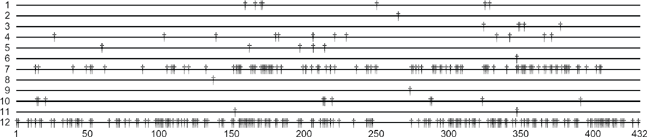
Identified polymorphic positions in first four levels of the Enolase tree.

To summarize, we have observed that many of the active site annotations in Uniprot for the Enolase dataset are present in prominent positions in our tree. Moreover, the tree makes suggestions for new annotations on two levels: it identifies possible new active sites, and it identifies new sequences that contain a known active site. We estimate that both types of information can be valuable for biological analysis.

Relation to existing methods

Our method fits in the framework of phylogenomic analysis ²² methods. In the context of subfamily prediction, these methods construct a hierarchical or phylogenetic tree over the entire family, starting from a multiple sequence alignment (MSA), and then extract subfamilies from the tree.

Bête ²³ was the first algorithm to automatically decompose a protein family into subfamilies. The method was later extended to include a module for classification of novel sequences into subfamilies and is better known under the name SCI-PHY. ¹¹ We discussed SCI-PHY in detail earlier and used it as reference in the experiments. We adopted its use of encoding cost to cut the hierarchical tree produced by our method.

Our method assumes that the size and diversity of the sequences allow an alignment of good quality. If this does not hold (due to high subfamily diversity, for example), it might be the case that the conserved positions within subfamilies are not well aligned; as a result, our method might not be able to find the appropriate splits to identify the subfamilies. A possible solution is to reconstruct the alignment after each split. However, this complicates classification of new sequences and functional site analysis. The idea of recomputing the MSA is similar in spirit as the GeMMA algorithm, ¹⁵ which was designed to deal with large and diverse protein families, where an accurate global MSA becomes infeasible. It applies a bottom-up clustering procedure and, after each merging step, recomputes an MSA for the sequences in the newly generated cluster. In order to decide which clusters to merge, a comparison score between alignments is computed. The scores are also thresholded to obtain a stopping criterion. The performance of GeMMA was shown to be comparable to SCI-PHY. ¹⁵ Albayrak et al ²⁴ proposed a method that avoids using an MSA altogether. Instead, it uses a relative complexity measure (RCM) to construct a pairwise distance matrix and constructs a NJ tree with it. The authors do not extract clusters from the tree but rather evaluate the tree topology. The results were comparable to those given by NJ trees using MSA.

To the best of our knowledge, no top-down phylogenomic method has previously been proposed for protein subfamily identification. Furthermore, top-down clustering approaches have rarely been used in biological applications in general. Varsharvsky et al ²⁵ point out three reasons for this: there is much more software available for bottom-up clustering, bottom-up clustering has an intuitive appeal, and it tends to generate topologies with high reliability at the more specific levels. On the other hand, Varsharvsky et al show that top-down clustering can be successfully applied to biological data.

Finally, our idea of using conserved positions to define subfamilies is related to the work of Bickel et al. ² Their main goal is to identify functionally related sites in a MSA. To that aim, they first enumerate all possible protein subfamilies that are defined by having at least two positions with subfamily-specific residues. Afterwards, they prune the list of potential functional sites and corresponding protein subfamilies by assessing the degree of association between these sites for each subfamily.

The main difference between the method proposed by Bickel et al and ours is that our method constructs a tree (ie, finds a complete and nonoverlapping set of subfamilies), whereas Bickel et al discover each subfamily independently, possibly resulting in an incomplete or overlapping set of subfamilies. In fact, if Clus would only consider single-amino-acid tests and only consider splits defined by at least two such tests, the (unpruned) list of subfamilies found by Bickel et al would correspond to the splits considered by Clus at the root node.

Note that requiring subfamily-specific residues is a stronger condition than requiring that a residue is conserved within a subfamily. In the latter case, the residue could still appear outside that subfamily. Consider, for instance, the tree displayed in Figure 3, and suppose there was only one test p16 = W in the node that splits subfamilies 4 and 5. Then subfamily 4 could only be identified by Bickel et al if position 16 had a non-W residue in all sequences outside of subfamily 4, whereas for Clus, a W might also appear in any sequence outside of subfamilies 4 and 5.

Conclusion

In this article, we investigated the use of a divisive conceptual clustering algorithm for protein subfamily identification. The proposed method clusters protein sequences not only based on their overall similarity but also based on the presence of conserved amino acid residues. It first builds a hierarchical tree using tests based on polymorphic positions to split the sequences and then uses a postpruning procedure to extract the predicted subfamilies from the tree. The polymorphic positions used to split the sequences result in a candidate list of functionally important sites. Moreover, new family members can easily be classified into one of the predicted clusters, by sorting them down the tree and checking the corresponding internal node tests.

We evaluated the proposed method on eleven datasets, and we compared its results with those of the phylogenomic method SCI-PHY. Next to analyzing the predicted clusters, we also analyzed the underlying tree, for which we proposed two intuitive measures. Furthermore, we compared the classification results given by the tree output by our method with those given by profile hidden Markov models, and we compared the mutations that occur in the tree to known functional site annotations for one dataset.

We have shown that (1) using splits based on polymorphic positions results in trees that are highly discriminating between subfamilies, (2) the tree topologies produced our method have a better quality than the SCI-PHY trees, (3) our method produces a protein subfamily clustering at least as good as the ones predicted by SCI-PHY and with the advantage of having in general a lower number of singleton clusters and a larger percentage of sequences in pure clusters, (4) the underlying decision tree classifies new sequences nearly as good as profile hidden Markov models, and (5) there is evidence that the tree can identify active sites.

All these results are arguments in favor of using the proposed method for automated protein subfamily identification.

As future work we plan to develop a visualization tool that will provide a user-friendly interface for the analysis of the candidate list of functionally important sites.

Author Contributions

Conceived the proposed method: EPC, CV, HB. Designed the experiments: EPC, CV, HB. Analyzed the data: EPC, CV. Wrote the first draft of the manuscript: EPC, CV. Contributed to the writing of the manuscript: EPC, CV, HB. Agree with manuscript results and conclusions: EPC, CV, HB. All authors reviewed and approved of the final manuscript.

Funding

EPC is supported by project G.0413.09 “Learning from data originating from evolution”, funded by the Research Foundation–-Flanders (FWO-Vlaanderen). CV is a Postdoctoral Fellow of the Research Foundation–-Flanders (FWO-Vlaanderen).

Competing Interests

Author(s) disclose no potential conflicts of interest.

Disclosures and Ethics

As a requirement of publication the authors have provided signed confirmation of their compliance with ethical and legal obligations including but not limited to compliance with ICMJE authorship and competing interests guidelines, that the article is neither under consideration for publication nor published elsewhere, of their compliance with legal and ethical guidelines concerning human and animal research participants (if applicable), and that permission has been obtained for reproduction of any copyrighted material. This article was subject to blind, independent, expert peer review. The reviewers reported no competing interests.

Supplementary Files

Figure S1. Clus-MinLength edited tree for the EXPERT dataset Enolase.

Figure S2. SCI-PHY edited tree for the EXPERT dataset Enolase.

Figure S3. NJ edited tree for the EXPERT dataset Enolase.

Figure S4. Clus-MinLength-ECC tree for the EXPERT dataset Enolase.

Figure S5. SCI-PHY tree for the EXPERT dataset Enolase.