Influence of Modularity and Regularity on Disparity of Atelostomata Sea Urchins

Abstract

A modularity approach is used to study disparity rates and evolvability of sea urchins belonging to the Atelostomata superorder. For this purpose, the pentameric sea urchin architecture is partitioned into modular spatial components and the interference between modules is quantified using areas and a measurement of the regularity of the spatial partitions. This information is used to account for the variability through time (disparity) and potential for morphological variation and evolution (evolvability) in holasteroid echinoids. We obtain that regular partitions of the space produce modules with high modular integrity, whereas irregular partitions produce low modular integrity; the former ones are related with high morphological disparity (facilitation hypothesis). Our analysis also suggests that a pentameric body plan with low regularity rates in Atelostomata reflects a stronger modular integration among modules than within modules, which could favors bilaterality against radial symmetry. Our approach constitutes a theoretical platform to define and quantify spatial organization in partitions of the space that can be related to modules in a morphological analysis.

Introduction

In general evolutionary discourse, the notion of “disparity” is used to express morphological diversity and body plan variety ¹ and it is a pragmatic concept used to define the degree of physical change in a biological entity although no theory accounting for the genesis of that change is available. Phenotypic variation provides substantial raw material for natural selection and evolution but few empirical data exist about the factors controlling this morphological variation or disparity, ² which could be useful to establish a conceptual platform to predict the shape of the organism in evolution. Even so, disparity may provide insights about the relationship between form and evolution and has been a rich source of study. Recently, the concept of modularity was applied to study cranial disparity in Primates and Carnivora; ² modules were defined as sets of highly correlated traits and it was concluded that strong integration between modules constrain morphological evolution in the placental skull.

In a modular approach, it is assumed that organisms are composed by individual entities or modules, and knowledge of modules and their integration is important to understand some properties of these organisms. Modularity might be seen as a tool to unveil features of the way organisms are build, as a consequence of an organizational principles of self-maintaining systems, ³ or of an “evolved property”. ⁴ The identification of structural and architectural modules is often a straightforward matter, ⁵ for instance, it has been pointed out that “the parts and characters routinely identified by the morphologist reflect hypotheses of modularity based on observational or quantitative criteria, without reference to the generative mechanisms or the theoretical contexts to which modules relate”. ¹ Progress in computational power has revealed that, in the light of genetic structural interactions, modularity, robustness, and evolvability are tightly related, with an intermediate degree of modularity allowing for a compromise of high robustness and high evolvability which otherwise are negatively related.^6–8 The analysis of abstract entities into constituent elements, and their degrees of interaction among internal parts, represents a source of important information in terms of robustness and evolvability. Alberch ⁹ set up the problem for the Modern-Synthesis-type view of the genotype–phenotype relationship by reminding biologists that genes do not specify development, and much less organismal form. The result of Alberch's line of inquiry is rather encouragingly converging with modularity, because it points out the value of functional integrity of modules beyond assumptions from old-fashioned metaphors-like genetic blueprint and genetic program which bypass development to genes determining phenotypes (see Ref. ¹⁰ and references therein).

In a previous work, ¹¹ we proposed a measurement of regularity of sea urchins and studied its changes of regularity in a macroevolutive and taxonomic level. In that work, it was highlighted that deviations from regularity were measured in Holasteroida order at particular geological times. In this work, we retake this observation and show that this departure from regularity is related with disparity of sea urchin belonging to the Atelostomata superorder (Holasteroida order belongs to this superorder). For this purpose, we use modularity in a pure geometrical context, which combined with regularity yields measurements of disparity of sea urchin belonging to this superorder that fits quite well independent values based solely on morphometric measurements. For this goal, a particular partition of the pentameric sea urchin body plan into five modules is proposed using Voronoi tesselations. A statistical analysis of the areas covered by each module, as compared with regular and irregular pentameric partitions of the plane (which are defined using measures of eutacticity), leads to quantify the spatial organization and the degree of interaction between modules. In a general context, our aim is the analysis of the pentameral body plan partition defined by modules and the study of the interaction between these modules, to establish a plausible hypothesis about geometrical space partitions and its implications for evolvability and disparity during evolution. This approach establishes a theoretical platform to study and quantify spatial organization in partitions of the space that can be related to modules in morphological analysis. From our results, it is concluded that more regular partitions (as measured by eutacticity) produces modules with low area variability, which is interpreted as high modular integrity. On the contrary, irregular partitions produce modules with high area variability, interpreted as low modular integrity (for an illustration see Fig. 6). This high or low modular integrity (and consequently high or low regularity) is further used to quantify the disparity observed in the Atelostomata superorder. Once the modular integrity was associated with regularity, disparity data in Atelostomata sea urchins reported by Eble ¹² are compared with measurements of regularity in our Atelostomata sample and a quite good fit is obtained.

This study is organized into four sections. In Section 2, previous general results concerning the geometrical analysis of phenotype during sea urchin evolution, using regularity as a mathematical tool, are reviewed including the mathematical framework. In Section 3, we establish our modular approach and its link with regularity. In Section 4, the numerical procedure to define modules in body plans of sea urchins is developed and results are presented in Section 5. Finally, discussion and conclusions are presented in Section 6.

Regular and Irregular Sea Urchins

Sea urchins are pentameric (fivefold partitioning) organisms with an apical structure, called the apical disc, ¹³ which includes five ocular plates (OP), shown in Figure 1, reflecting the global body plan of Echinodermata. In a previous work, we showed that OP is useful to quantify the degree of regularity of echinoids by using a set of vectors with the same origin (vector star) pointing to each of the OP ¹¹ and measuring the regularity (eutacticity) of this vector star. With this approach, measures of regularity and its changes were carried out in that work in a collection of 157 extinct and extant sea urchins. Results suggested a high degree of regularity in the shape of sea urchins through their evolution; rare deviations of regularity were measured in Holasteroida order. ¹¹ At this point, since the observed departure from regularity seems to constitute a critical evolutive event in sea urchins, ¹⁴ we retake this geometrical approach here, looking to relate geometrical measures of regularity with disparity rates and evolvability using modularity. Disparity data in echinoids reported by Eble ¹² will be used to test our results.

Figure 1.

Apical disc (encircled) showing landmarks (numbered) at ocular plates. The star vector is formed by vectors pointing to these landmarks, with a common origin at the center of mass.

For completeness, and to fix notation, in what follows, we resume the main definitions concerning eutactic stars. A star vector, or simply, a star in the plane (R ² ), is a set S of N vectors in R ² , with a common origin and N > 2, S = {u₁, u₂,…, u _N }. The star S is said to be eutactic if it can be obtained by projecting an orthogonal set of N vectors {U₁, U₂,…, U _N } in an N-dimensional space (R^N). Eutacticity is closely linked with regularity since a given polygon, polyhedron and, in general, polytope can be associated with a star of vectors (pointing to the center to the vertices) and it has been demonstrated that stars associated with regular polygons, polyhedra or, in general, polytopes, are eutactic. ¹⁵ Thus, we have used this fact to propose that a measure of eutacticity provides a measure of regularity of shapes that can be associated with a star, as is the case of sea urchins. ¹¹

A reliable numerical criterion for the eutacticity of a star, suitable for working with experimental measurements, was proposed in Ref. ¹⁶ and is as follows. Let A be the matrix whose N columns are the components of the vector composing a star S, with respect to a given fixed orthonormal basis of R ² . Then, a star S in R ² , represented by the matrix A , is eutactic if and only if ¹⁶

$$\epsilon \equiv \frac{\text{Tr}\left(\text{S}\right)}{\sqrt{\text{Tr}\left(\text{SS}\right)}\sqrt{2}}=1,$$

(1)

where S = AA ^T ; Tr denotes the trace and the superindex T denotes the transpose. Notice that the parameter ∊ is capable f indicating the degree of eutacticity of the star represented by A : if it is not strictly eutactic (∊ = 1), then this quantity is closer to 1, the more eutactic the star is. In our particular case of planar stars, it can be proved that ¹⁶

$$\frac{1}{\sqrt{2}}\le \epsilon \le 1.$$

(2)

As already mentioned in Ref. ¹¹ , the strategy was to associate a particular echinoid with a star and measure its eutacticity by means of Eq. 1; the more closer the value of ∊ to 1, the more regular the star (and the echinoid) is. In that work, regularity (eutacticity) of sea urchins through geological time was analyzed using the family taxonomic level in a collection of 157 extant and extinct sea urchins. It was reported that regularity has dominance over irregularity in sea urchins evolution; despite that variability increases over time, statistically sea urchins show a high degree of regularity. The lowest values of regularity were recorded first in early Mesozoic Collyritidae and these low values continued for late Mesozoic and Cenozoic Holasteridae, Portuolesidae and Corystidae (Fig. 5 in Ref. ¹¹ ). An interesting fact is that all these families belong to the Holasteroida order (Atelostomata superorder), which seems to constitute a critical evolutive event in sea urchins evolution. ¹⁴ Most living representatives of Holasteroida are deep-water inhabitants with exceedingly thin and fragile tests. This departure of regularity will be studied in what follows, by adopting an approach based on modules and its interactions. As we will see, with this approach regularity with modularity is linked to provide not only a description of visible modules and their interactions, but also established plausible hypothesis with implications for studying disparity and evolvability in this order.

Modularity and Regularity

In a modular approach, modules are recognized by two aspects: (1) autonomy from other modules or traits and (2) strong integration of traits within the module. ² Thus, geometrically, with certain parts of a system (a vertex or a landmark), we can associate a spatial fragment with a module, provided that it is composed of a set of highly and weakly correlated traits outside the module.

Modularity itself also evolves, and new schemes for modularity may arise by the fragmentation of a large group of traits into smaller groups by severing interactions, bridging new groups of modules.^4,17 The modules can then vary independently of each other by releasing modular integrity, facilitating the “evolvability” of the system, that is, its potential for morphological variation and evolution. Such a dissociation mechanism has been suggested to be a process that counteracts developmental canalization which would otherwise increase over evolutionary time and affect the generation of variation. ⁴ In the theory of modules, spatial organization in the sense of modular integrity results in a fruitful concept. Spatial organization for entities in a system reflects interactions between parts and can be interpreted as physical contiguity, thus implying territory invasion; if the potential space to be used is well distributed, less interference is expected. The larger the variability of spatial entities, the more interference between contiguous parts results from inequalities in space distribution.

Sea urchins have a pentameral readily visible body plan, with radial or bilateral symmetry; in such a partition, five modules can be clearly associated to the five ambulacral (or interambulacral) zones. Since we will just be dealing with geometric properties, the identification of these modules can be justified in terms of a homogeneous partition of the space. Indeed, the following facts concerning the coronal morphology of sea urchins are well known (Ref. ¹⁸ and references therein): (a) ambulacral and interambulacral zones are composed by plates defining polygonal patterns; (b) at metamorphosis, each ambulacrum and interambulacrum usually has two to four plates that have grown together to form the polygonal mosaic; and (c) existing plates continue to grow by peripheral accretion and new plates are added at the edge of the apical system. Therefore, we assume that the basic principle behind the formation of the ambulacral and interambulacral zones is that the available space is partitioned in a homogeneous way to allow the formation of polygonal mosaics of plates without interference between zones. This partition is thus defined by modules.

With this idea, our strategy is to relate measurements of eutacticity (regularity) with those of spatial organization in sea urchins body plans. The aim is an analysis of space partitions to consider not only the geometrical description of visible modules (or parts with several degrees of interference) but also their interactions. Our hypothesis is that the higher the eutacticity, the more homogeneous the space partition or the lower area variability (as illustrated in Fig. 6(a)); lower values of eutacticity imply unequal partition of the space or more area variability (as illustrated in Fig. 6(b)).

Methods

As a first step, we should describe a procedure to define modules in the sea urchin architecture. Since spatial organization is the main property to consider, a partition of the pentameric sea urchin body plan in modules is proposed using Voronoi tessellations (for an introduction to Voronoi tesselations, see for instance Chapter 2 of Ref. ¹⁹ ), according to the following geometrical algorithm (see Fig. 2):

Figure 2.

Algorithm used to associate modules to a given vector star. (A) – (D) correspond to steps 1, 2, 3, and 4, respectively, of the algorithm described in Section Methods.

1. 1.

   A random star S of N vectors, S = (u₁, u₂,…, u _N }, is generated inside a circle of radius R. As we will see below, a set of regular stars (∊ = 1) and a set of irregular stars (∊<0.8; see justification below) will be generated, for N = 3, 4, 5, 6, and 7.

2. 2.

   In this circle, a set of P randomly generated points is inscribed, with the restriction that no two points of the set S + P are closer with a certain distance r.

3. 3.

   The Voronoi tessellation associated with the set of points S + P is calculated.

4. 4.

   The Voronoi tessellation obtained in the previous step is partitioned as follows. Given a vertex u _i of the star S, the set of Voronoi polygons that are closer to u _i than to any other vertex u _j (j ≠ 1) are selected; this process is repeated for each vertex u _i (i = 1, 2,…, N). Thus, the Voronoi tessellation is partitioned into N sub-tessellations or modules L₁, L₂,…, L_N.

Let A_i be the total area of the Voronoi polygons associate with the module L_i. Now, our main goal will be to study the variation of total areas between modules L₁, L₂,…, L_N, for partitions associated with regular and irregular stars; the larger the variation, the less homogeneous the partition of the space is. In order to support the statistics, for each star Σ, generated at step 1, M sets of random points, P₁, P₂,…, P_M, are generated and for each set, steps 2, 3, and 4, of the above procedure, are applied. Now, for a given N (the number of vectors of the star S), E random regular stars, S₁, S₂,… S_E, are generated and the same number of irregular stars and the procedure already described is applied for each case. Therefore, let A_aj^e be the area of the module L_m of the star S_e, corresponding; to the set of random points P_j, then the mean area of the module L_m is

$${\overline{A}}_m=\frac{1}{M\times E}\sum _{e=1}^E\sum _{j=1}^M{A}_{mj}^e$$

(3)

and the standard deviation of the E average areas corresponding; to the module L_m is

$${\sigma }_m=\sqrt{\frac{1}{M\times E}\sum _{e=1}^E\sum _{j=1}^M{\left(A_{mj}^e-{\overline{A}}_m\right)}^2}$$

(4)

Some details about numerical issues involved in the four-step algorithm described above should be stated before proceeding. In step 1, regular and irregular random stars are generated in the following way. First, we consider bilateral stars such that the free parameters are the size of the vectors in the right hand size of the star and the angle with respect to the x axis (see Fig. 3 for the case of pentagonal stars); vector sizes are chosen randomly in the range [1,R] and angles are equally chosen randomly in the range [0,π/2]. Once a random bilateral star is generated, a regular star (∊ = 1) is obtained by calculating the “closest” eutactic star to the given star by following the procedure described in Ref. ²⁰ For generating an irregular star, we should introduce values of ∊ defining irregular stars; in Ref. ¹¹ , we reported that rare deviations of regularity in the shape of sea urchins through the evolution were found with values of 0.8 and below, thus we simply calculate ∊ (see Eq. 1) to the generated random star and if this value lies in the numerical range [0.71,0.8] then it is considered, otherwise, a new random star is generated until the desired value is attained. In step 2, coordinates (x_i, y_i) are randomly generated inside the circle of radius R; if a generated point is closer than r to an already generated point, it is discarded and a new point is randomly generated, which is also subjected to the same closeness test. In step 3, Voronoi tessellations are calculated using the Computational Geometry package of the commercial software Mathematica; to avoid non-representative data during the calculation of Voronoi tessellations, polygons with at least one vertex outside the convex hull were removed. In step 4, it may occur that a point of a given Voronoi polygon is closer to a vertex u _i but another point of the same polygon is closer to a different vertex u _j . If this is the case, the polygon is discarded from the analysis and this is why a separation between modules is clearly seen in Figure 2(d).

Figure 3.

Geometrical parameters required to replicate random bilateral stars. The pentagonal star is used as example but vector magnitudes (lowercase letters) a, b, c, etc., and angles (Greek letters) α, β, δ, γ, etc., may increase or decrease according to the number of vectors.

Results

Stars with the number of vectors N = 3, 4, 5, 6, and 7 were generated, and in all cases, sets P_i (i = 1, 2, M) with 300 uniformly distributed pseudo-random points were generated. Other parameter values are E = 100, M = 100, R = 3, and r = 0.5. As already mentioned, E is the total size of random regular stars, M is the total size of pseudo-random points, R is the radius of the circles were the pseudo-random points are inscribed, and r is the minimal allowed distance between pseudo-random points.

Area Variability between Modules

The null hypothesis is that the standard deviation corresponding to modules defined by regular stars is similar to that resulting from irregular stars.

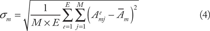
Notice that we can get an estimation of the area variability of the module L_m by using the average of the standard deviation of σ _m (given by Eq. 4), denoted by $\stackrel{-}{\sigma }$ _m and calculated as follows. Fix N, the number of vectors of the stars, and let $\stackrel{-}{A_m{}^e}$ be the area of the module L_m corresponding to the star e, averaged over the M sets of random points P₁, P₂, …, P_m, that is:

$${\overline{A}}_m^e=\frac{1}{M}\sum _{j=1}^M{A}_{mj}^e,$$

(5)

To this average, the corresponding standard deviation is given by

$${\sigma }_m^e=\sqrt{\frac{1}{M}\sum _{j=1}^M{\left(A_{mj}^e-{\overline{A}}_m^e\right)}^2.}$$

(6)

Therefore, for a given star S_e, it corresponds to the standard deviation σ_m^e of the areas corresponding to the module L_m. Since we have generated E stars, the average of the standard deviations can be obtained as

$${\overline{\sigma }}_m=\frac{1}{E}\sum _{e=1}^E{\sigma }_m^e.$$

(7)

Taking this value as an estimation of the area variability of module L_m, we performed an ANOVA to detect statistically significant differences on area variability of modules defined either by regular or irregular stars. In Figure 4, it can be observed that the area variability in modules defined by irregular stars is considerably larger. This statistical difference is more noticeably when all the modules (3+4+5+6+7) are compared; in this case, the null hypothesis is rejected in 23 of the 25 modules, with a statistical significance p ranging from less than 0.0001 for partitions with three modules; less than 0.001 for partitions with four modules; less than 0.05 for partitions with 5 modules; and less than 0.01 for partitions with 6 and 7 modules. Consequently, the area variability of modules obtained from regular stars is different than those obtained from irregular stars. Even more, regular stars yield modules with lower variability than modules coming from irregular stars. It should be pointed out that our experiment fails in the cases of modules L₁ in partitions with 3 modules (Fig. 4(a)) and L₄ in partitions with 4 modules (Fig. 4(b)). In both the cases, no statistically significant differences between partitions coming from either regular or irregular stars were observed.

Figure 4.

ANOVA of differences of area variability, that is $\stackrel{-}{{\sigma }_m}$ (see Eq. 6), for regular and irregular partitions of the space. Partitions with (A) three modules, (B) four modules, (C) five modules, (D) six modules, and (E) seven modules, p-value thresholds of the ANOVA are in the top right panel.

Notice that from our results, it turns out that if ${\overline{\sigma }}_m$ provides information about the variability of the area of modules, then the standard deviation of this mean contains the information about the overlap (interaction) between modules. By calculating this standard deviation (error bars in Fig. 4), we obtain that structures with modules defined by irregular stars have large values, thus implying large interference between modules which can be related with low modular integrity (see Fig. 6(b) for an illustration). On the contrary structures with modules defined by regular stars have small values of standard deviations; thus, small interference between modules is measured, implying larger modular integrity (see Fig. 6(a) for an illustration).

Disparity and Regularity

From the previous results, we concluded that regularity implies modular integrity since results in Figure 4 can be interpreted as implying that modular contiguity increases when regularity decreases. On the other hand, it is accepted that modular organization favours evolvability by allowing one module to change without interfering with the rest of the organism. ²¹ Therefore, since we can measure regularity in our Atelostomata sample, to tests our results so far we need an independent measure for disparity in this clade.

Eble ¹² established a formal approach to measure disparity using morphometric tools in sea urchin evolution. For that goal, he first introduced a code for stratigraphic intervals, which is as follows: j1 = Aalenian–Bajocian, Middle Jurassic; j2 = Bathonian–Callovian, Middle Jurassic; j3 = Late Jurassic; k1 = Neocomian, Early Cretaceous; k2 = Barremian–Aptian, Early Cretaceous; k3 = Albian, Early Cretaceous; k4=Cenomanian–Santonian, Late Cretaceous; k5 = Campanian–Maastrichtian, Late Cretaceous and pal = Paleocene. For each defined interval, the corresponding disparity was calculated ¹² by considering a 38-dimensional landmark-based morphospace representing the test architecture. This morphometric analysis is used by Elbe to describe morphological evolution in terms of total variance and total range.

In Table 1, the results by Eble about Atelostomata superorder are summarized in the second column. The numerical values were obtained by digitizing the first of the Figures 4 of Ref. ¹²

Table 1.

Stratigraphic intervals coded as in Ref. ¹² , for species belonging to Atelostomata superorder studied in this work. Its corresponding disparity values (second column) were taken from the same Reference, and regularity data (third column) were obtained from our numerical calculations, as well as the corresponding standard deviation.

CODE 12	DISPARITY 12	REGULARITY MEAN	STANDARD DEVIATION
j2	19.7	0.859	0.196
j3	22.5	0.859	0.196
k1	33.5	0.908	0.128
k2	30.0	0.905	0.092
k3	33.5	0.928	0.073
k4	37.0	0.937	0.068
k5	36.0	0.934	0.075
pal	31.0	0.930	0.087

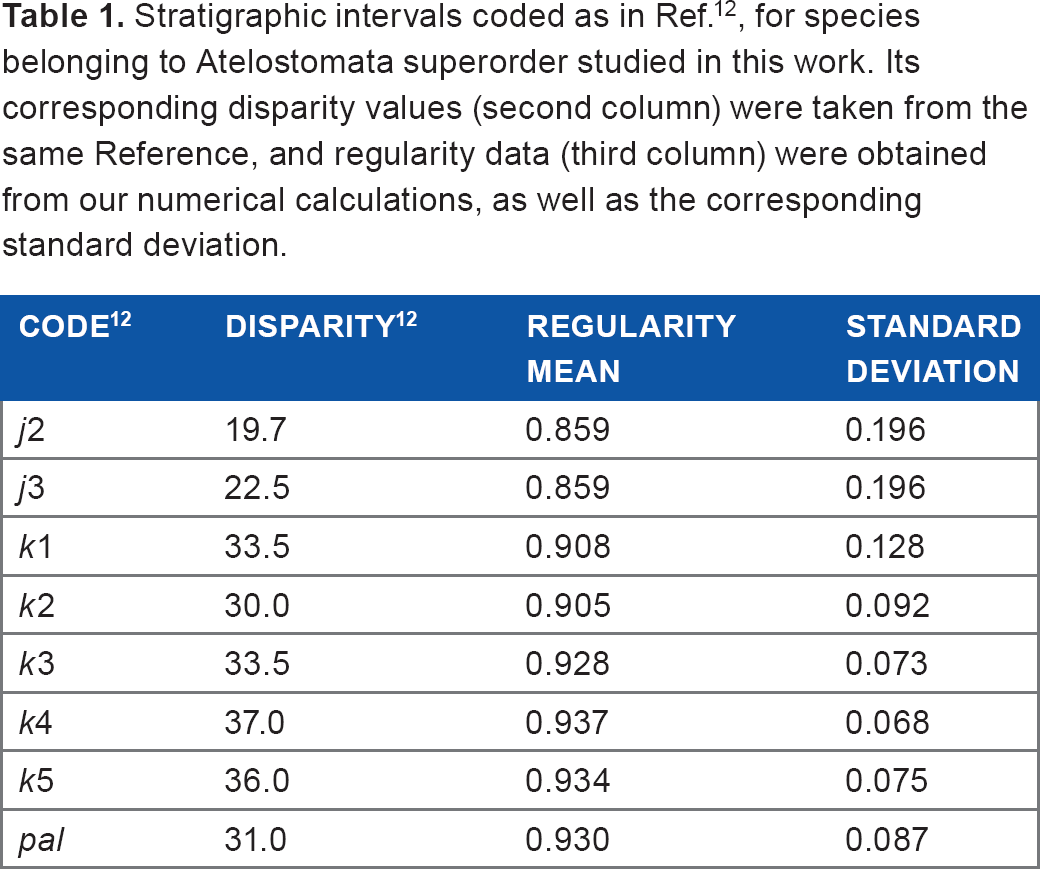
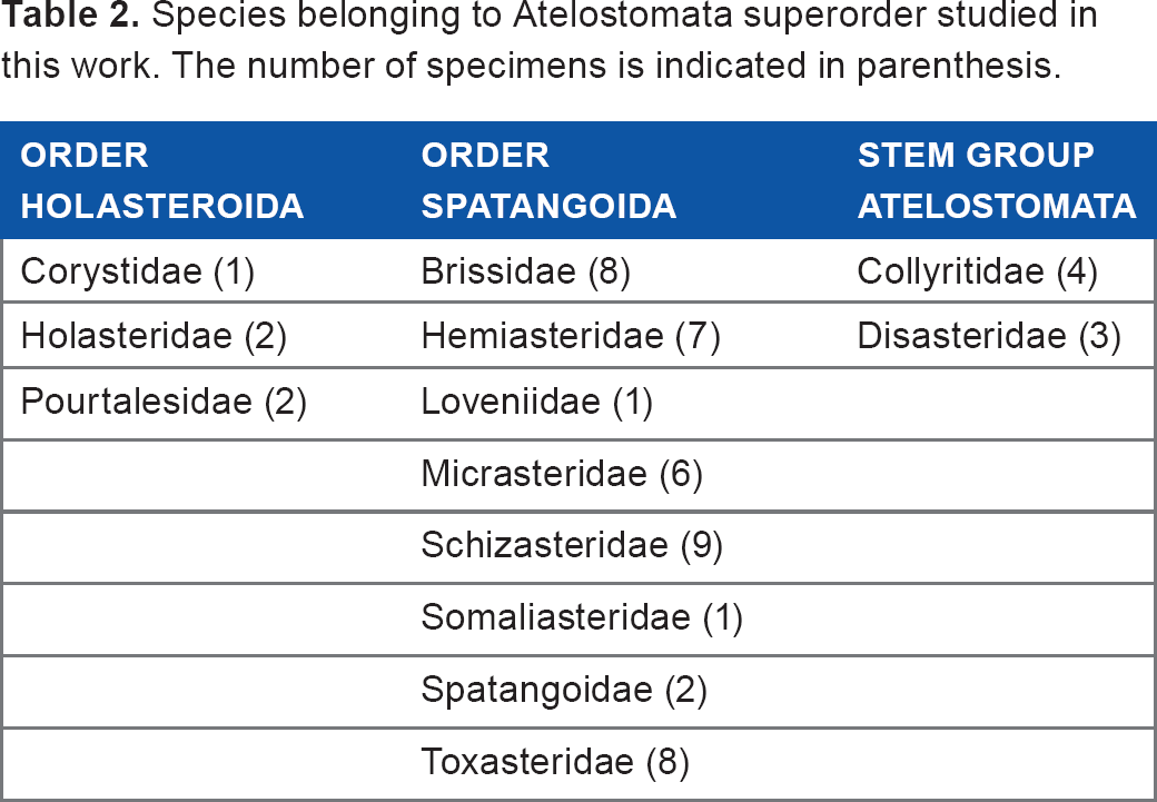
From the specimens studied in Ref. ¹¹ we pick those belonging to the Atelostomata superorder (see Table 2). These 54 species were classified according to their stratigraphic intervals using Eble's code ¹² (notice that, for instance, the range of Brissidae is from Eocene to recent). For each specimen belonging to a given stratigraphic interval, its value of regularity, according to (1), was calculated and the mean is displayed in the third column of Table 1, with its corresponding standard deviation in the fourth column. Notice that the row corresponding to j1 is not included since none of the studied specimens belongs to this stratigraphic interval.

Table 2.

Species belonging to Atelostomata superorder studied in this work. The number of specimens is indicated in parenthesis.

ORDER HOLASTEROIDA	ORDER SPATANGOIDA	STEM GROUP ATELOSTOMATA
Corystidae (1)	Brissidae (8)	Collyritidae (4)
Holasteridae (2)	Hemiasteridae (7)	Disasteridae (3)
Pourtalesidae (2)	Loveniidae (1)
	Micrasteridae (6)
	Schizasteridae (9)
	Somaliasteridae (1)
	Spatangoidae (2)
	Toxasteridae (8)

In Figure 5(a), the values of our measured values of regularity average (third column in Table 1) are plotted versus Eble's disparity rates (second column in Table 1), for its corresponding stratigraphic intervals; a high positive correlation is found (r = 0.946). In contrast, in Figure 5(b), the regularity standard deviation (fourth column in Table 1) are plotted versus Eble's disparity rates, where a high negative correlation is found (r = −0.914), which confirms our numerical results that the value of regularity is an indicator of modular integrity.

Figure 5.

(A) Mean regularity (third column in Table 1) plotted versus Eble's disparity rates (second column in Table 1), for its corresponding stratigraphic intervals; a high positive correlation is found, displayed on top of the graph. (B) Regularity standard deviation (fourth column in Table 1) plotted versus Eble's disparity rates, where a high negative correlation is found, also displayed on top of the graph.

Discussion

Phenotypic evolvability should not be taken for granted, it requires an explanation that must come from a theory of organismal variation. ²¹ In this work, we showed that eutacticity as a measure of regularity also implies a measure of spatial organization which may turn into a measure of phenotypic variation. Modular organization favors evolvability by allowing a module to change without interfering with the rest of the organism (see, for instance, Refs.^17,22). Irregular stars produce partitions with high variability in areas and thus low degree of independence between spatial modules (ie, interference; see Fig. 6(b) for an illustration). Modules with a high degree of independence have low interference with their neighbors, which is expressed as low variability (standard deviations in Table 1) of areas for values of eutacticity around 0.93704 in Atelostomata superorder (see Fig. 6(a) for an illustration). Therefore, it is useful to contrast high regular modules with modules with low regularity in order to provide insights on the implications of modularity in organismal variation reflected as disparity. In Atelostomata superorder, the resulting modular structure tends to show less cohesion among modules (inter modular independence) than within modules (intra modular cohesion) which produces a high potential to change (evolvability). This is expressed in the disparity measurements shown in Figure 5, where k4 shows an increase in morphological diversity during Cenomanian–Santonian ages in the late Cretaceous. The correlation analysis between regularity mean and disparity shows a positive relationship (r = 0.946) between the increasing of eutacticity values with the increasing of disparity rates.

Figure 6.

Scheme for area variability of modules defined by regular stars (A) versus modules defined by irregular stars (B) ones. In case (A), low variability in areas (standard deviations) is depicted; this low variability implies non-significant overlap between modules, that is, high within-module integrity. On the contrary, in case (B) high variability in areas (standard deviations) is depicted; it implies significant overlap between modules and low within-module integrity.

According to Goswami and Polly, ² two hypotheses should be considered when dealing with the evolutionary implications of modularity: (a) the constrain hypothesis predicting that highly correlated modules (strong inter-module cohesion) should display low morphological disparity and (b) the facilitation hypothesis that predicts high intra-modular integration with high morphological disparity. Our model of spatial organization concludes that irregular arrangements imply a decrease in disparity by low integration inside modules with high spatial interference among modules or body plan fusion (see Fig. 6(b) for an illustration), thus supporting the facilitation hypothesis. It seems likely that inter module spatial interference constrains the evolution of pentameric radial shape yielding the establishment of two modules instead of five, and high intra-modular integration facilitates high rates of disparity in Atelostomata superorder even when they are bilateral. On the other hand, pre Triassic-Jurassic sea urchins forms have values of eutacticity close to one. ¹¹ According to our results, a possible implication of this high regularity is that disparity may have achieved high rates during the first ages of sea urchin evolution. In that sense, despite that the variability of eutacticity measurements increases over time, sea urchins remain with a high degree of regularity during evolution. ¹¹ In fact, radial sea urchins with regularity values close to 1 require further study in order to define disparity rates in non-Atelostomata clades.

It is worth to mention that the analysis and results presented here should also be considered as a motivation to continue with geometrical analysis for predicting the importance of spatial configurations for morphological diversification. Likewise, punctuated morphological innovations during evolution arose not just in the context of genetic variability and the functional selection of biological associated inputs from external ecological conditions, they may also come from releasing the internal ties given by geometry. Biological entities are provided by nature with particular features that are not found in less-complex physical systems since the level of complexity increase notably in biology. However, the evolutionary setup for biological systems shares also the most basic features with less-complex physical systems, such as, shape and structure. D'Arcy Thompson ²³ conceives those basic features as a source of potential knowledge to understand organismic transformations, providing them with geometrical features during the course of evolution.

Author Contributions

Jointly conceived the study and designed the numerical experiments: JLA, JL-S. Wrote codes and ran the numerical calculations: JLA. Jointly collected and analyzed data: JL-S, JM-B. Jointly supervised the project and developed the structure and arguments for the paper: AL-F, FS-M. Wrote the first draft of the manuscript: JL-S. All authors made critical revisions and approved final version. All authors discussed the results and implications and commented on the manuscript at all stages.