Sage Journals: Discover world-class research

Abstract

A multilinear reference tissue approach has been widely used recently for the assessment of neuroreceptor–ligand interactions with positron emission tomography. The authors analyzed this “multilinear method” with respect to its sensitivity to statistical noise, and propose regularization procedures that reduce the effects of statistical noise. Computer simulations and singular value decomposition of its operational equation were used to investigate the sensitivity of the multilinear method to statistical noise. Regularization was performed by truncated singular value decomposition, Tikhonov-Phillips regularization, and by imposing boundary constraints on the rate constants. There was a significant underestimation of distribution volume ratios. Singular value decomposition showed that the bias was caused by statistical noise. The regularization procedures significantly increased the test–retest stability. The bias could be reduced by applying linear constraints on the rate constants based on their normal range. Underestimation of distribution volume ratios by the multilinear method is caused by its sensitivity to statistical noise. Statistical power in the discrimination of different groups of subjects can be significantly improved by regularization procedures without introducing additional bias. Correct distribution volume ratios can be obtained by imposing physiologic constraints on the rate constants.

Keywords

PET Modeling Linear regression Reference tissue method Regularization

Linear regression methods, also called graphical methods, are widely used for the quantification of reversible binding of radioligands to neuroreceptors in positron emission tomography (PET) and single-photon emission computed tomography (SPECT) imaging. Linear methods are appreciated because they can be easily applied on a voxel-by-voxel basis to generate parametric images of the brain. The most widely used linear method, the Logan plot (Logan et al., 1990), is an “invasive” approach in that it requires arterial blood sampling, which is an additional source of statistical and systematical errors and involves significant discomfort for most patients.

A new class of techniques suggests the replacement of the arterial input function by the time–activity curve (TAC) of a receptor-free reference region. These reference tissue methods significantly improve compliance of subjects. A reference tissue method characterized by a multilinear operational equation, and thus combining the advantages of reference tissue approaches and linear regression, was developed by Ichise et al. (1996, 2001). This method is subsequently referred to as the multilinear method.

The multilinear method has been increasingly used recently. For example, the method was used to determine serotonin transporter occupancy of (unlabeled) serotonin reuptake inhibitors during treatment in humans (Meyer et al., 2001, 2002). However, the sensitivity of the multilinear method to statistical noise has not yet been evaluated in detail.

Therefore, we analyzed the sensitivity of the multilinear method to statistical noise via singular value decomposition (SVD) of its operational equation in a typical PET patient study using the serotonin transporter ligand [¹¹C](+)McN5652 (Suehiro et al., 1993). Taking into account the rather low in vivo specific-to-nonspecific binding ratios in humans for most receptor ligands, reliable detection of small changes in receptor availability is of great importance. Therefore, stabilization of the multilinear method by different regularization procedures was also investigated.

MATERIALS AND METHODS

Multilinear method

The multilinear method (Ichise et al., 1996) can be derived from the well-known Logan plot for the graphical analysis of reversible radioligand binding (Logan et al., 1990, 2000; Patlak et al., 1983):

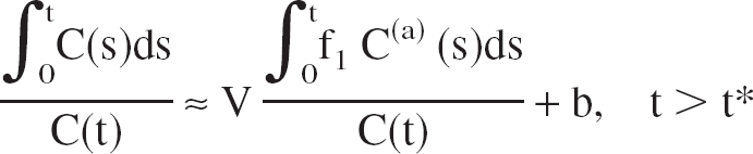
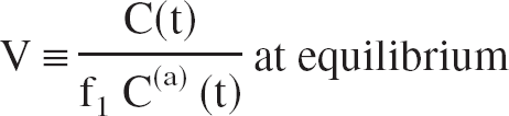
\frac{\int_{0}^{t} C (s) ds}{C (t)} \approx V \frac{\int_{0}^{t} f_{1} C^{(a)} (s) ds}{C (t)} + b, t > t^{*}

(1)

where C(t) is the TAC of the volume of interest (VOI), f₁ C^(a) (t) is the free fraction of the unmetabolized tracer in arterial plasma (input function), V is the total equilibrium DV of the tracer in the VOI, and b is (almost) constant at late times t > t*. The distribution volume V is defined as the equilibrium ratio of the tracer concentration in the VOI to the free arterial concentration:

V \equiv \frac{C (t)}{f_{1} C^{(a)} (t)} at equilibrium

(2)

Combining the Logan plot formula (Eq. 1) for two different tissue TACs, C(t) and C′(t), by solving the C′(t)-formula for the plasma integral, inserting the result in the C(t)-formula, and multiplying both sides by C(t) yields

\int_{0}^{t} C^{'} (s) ds R + C^{'} (t) (- R b^{'}) + C (t) b \approx \int_{0}^{t} C (s) ds, t > t^{*}

(3)

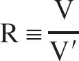
where the equilibrium DV ratio R is defined as the ratio of the total DVs in the two regions with concentrations C to C′:

R \equiv \frac{V}{V^{'}}

(4)

Equation 3 is the operational equation of the multilinear method. It is linear in R, b, and b′.

Within the two-tissue (2T) compartment model consisting of a nondisplaceable compartment, C₂, and a specific compartment, C₃, the total distribution volume V is the sum of the nondisplaceable equilibrium distribution volume, V₂, and the specific equilibrium distribution volume, V₃:

V = V_{2} + V_{3} and V^{'} = V_{2}^{'} + V_{3}^{'}

(5)

Fractional blood volume has been neglected. In terms of the rate constants:

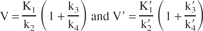
V = \frac{K_{1}}{k_{2}} (1 + \frac{k_{3}}{k_{4}}) and V^{'} = \frac{K_{1}^{'}}{k_{2}^{'}} (1 + \frac{k_{3}^{'}}{k_{4}^{'}})

(6)

where K₁ f₁ C^(a) is the tracer flux from arterial plasma to C₂, k₂ is the unidirectional rate constant for the loss of tracer from the tissue through C₂, and k₃ and k₄ are the rate constants for the tracer transfer from C₂ to C₃ and vice versa.

If C′ is assumed to represent a proper reference region for the receptor-rich region C:

reference region : V_{3}^{'} = 0 and V_{2}^{'} = V_{2}

(7)

one obtains from Eqs. 4 and 5:

R - 1 = \frac{V_{3}}{V_{2}} \equiv V_{3}^{″}

(8)

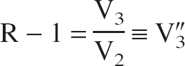
where R-1 is the so-called specific-to-nonspecific equilibrium partition coefficient, usually denoted by V″₃ (Laruelle et al., 1994). Within the 2T-compartment model, V″₃ is given by:

V_{3}^{″} = \frac{k_{3}}{k_{4}}

(9)

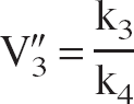
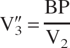
V″₃ is related to the binding potential (BP), defined as the ratio of the concentration of available receptors, B_max, to the equilibrium dissociation constant, K_D, according to (Laruelle et al., 1994):

V_{3}^{″} = \frac{BP}{V_{2}}

(10)

Note that for the DV ratio R to reflect the receptor density B_max, both K_d and V₂ must be constant between individuals and diseases (Ichise et al., 2001).

Data

[¹¹C](+)McN5652 has been previously shown to be one of the most appropriate tracers to quantify availability of the presynaptic serotonin transporter in vivo in the human brain (Buck et al., 2000; McCann et al., 1998; Parsey et al., 2000; Szabo et al., 1995, 1999). Time-activity curves from a typical [¹¹C](+)McN5652 PET patient study were provided by the commercial PMOD software package (Version 2.35 for Windows NT; Medical Imaging Software, Zurich, Switzerland; Mikolajczyk et al., 1998). Details on PET imaging and blood sampling have been described previously (Buck et al., 2000). From these data, metabolite-corrected tracer concentration in arterial plasma, C_i and TACs of a receptor-rich region (left thalamus), C_i, and a reference region (gray matter of left cerebellum), C′_i, were used (Fig. 1). The subscript i = 1, …, 31 refers to the individual time frames. The free fraction f₁ of [¹¹C](+)McN5652 in arterial plasma was set to 1 in the following analyses, which is of no concern for the present investigation.

FIG. 1.

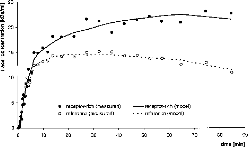
Positron emission tomography patient study using the serotonin transporter ligand [¹¹C](+)McN5652 showing time– activity curves (TACs) of a receptor-rich region (thalamus) and a receptor-free reference region (cerebellum). Measured TACs were taken from the [¹¹C](+)McN5652 example in the commercial software package PMOD. Model TACs were obtained from measured TACs by invasive quantification using the 2T-compartment model.

Data were first analyzed by the invasive 2T-compartment model, neglecting fractional blood volume, to yield model curves C͂_i and C͂′_i for the receptor-rich region and the reference region, respectively (Fig. 1). The multilinear method was then applied using both the measured TACs C_i, C′_i and the model TACs C͂_i, C͂′_i.

The operational Eq. 3 of the multilinear method was solved in the least-squares sense (Moore-Penrose solution) by SVD (Appendix). t* = 20 minutes p.i. was used (i.e. frames 21–31 were included in the fit).

Statistical noise

To simulate statistical noise, the number of radioactive decays within the receptor-rich region during frame i, Ñ_i, was computed according to the following equation:

{\tilde{N}}_{i} = ((1 - e^{- λ d_{i}}) / λ d_{i} / e^{λ s_{i}}) d_{i} W {\tilde{C}}_{i}

(11)

where W is the volume of the receptor-rich region (taken to be 3 mL), λ is the decay constant of ¹¹C, and s_i and di the start and the duration of the i^th frame, respectively. Then, Ñ_i was assumed to be a sample from a normal distribution with mean Ñ_i and standard deviation:

{SD}_{i} = ρ \sqrt{{\tilde{N}}_{i}}

(12)

The number of decays during frame i of the j^th dynamic scan, N_ij, was simulated according to the following equation:

N_{ij} = {\tilde{N}}_{i} + r_{ij} {SD}_{i}

(13)

where r_ij is a random matrix whose elements are normally distributed with mean 0 and variance 1. For a typical patient study, ρ = 100 is adequate (see below in this section). The radioactivity concentration C_ij corresponding to N_ij was obtained by inversion of Eq. 11. This procedure was applied to the model TAC of the reference region, C͂′_i, analogously (volume of the reference region W = 20 mL). Independent random matrices were generated for the receptor-rich region and the reference region. Figure 2 shows relative standard deviations of C͂_i and C͂′_i. Comparing the relative standard deviations of the simulated noisy TACs with the differences between measured TACs and modeled TACs (Fig. 1), the simulated noise levels appear realistic. A total of 10⁴ dynamic scans were simulated. The multilinear method was applied to each data set.

FIG. 2.

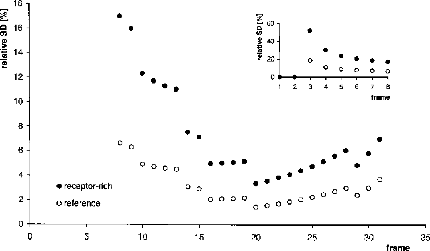
Simulation of statistical noise showing the standard deviation of tracer concentration relative to the mean tracer concentration (%). The scan protocol included 31 frames with a total acquisition time of 90 minutes using frame durations of 9 × 20, 4 × 30, 2 × 60, 4 × 120, 9 × 300, and 3 × 600 seconds (Buck et al., 2000). The standard deviation of the tracer concentration in the first two frames was set to 0 because the model time–activity curves vanished in these frames.

Singular value decomposition

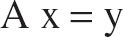
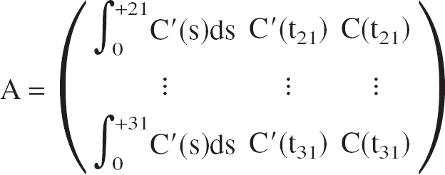
Using frames 21 to 31 of the TACs, the operational Eq. 3 reduces to a system of 11 linear equations with 3 unknowns, which can be written in matrix notation as:

A x = y

(14)

where A is the 11 × 3 coefficient matrix given by

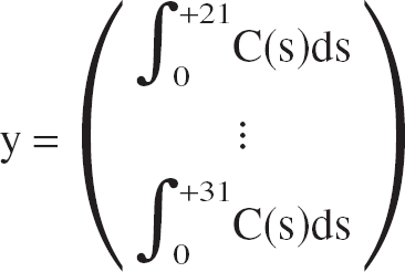
A = (\begin{array}{l} \int_{0}^{+ 21} C^{'} (s) ds & {C^{'} (t}_{21}) & {C (t}_{21}) \\ ⋮ & ⋮ & ⋮ \\ \int_{0}^{+ 31} C^{'} (s) ds & {C^{'} (t}_{31}) & {C (t}_{31}) \end{array})

(15)

y is the 11-dimensional right-side vector

y = (\begin{array}{l} \int_{0}^{+ 21} C (s) ds \\ ⋮ \\ \int_{0}^{+ 31} C (s) ds \end{array})

(16)

and × is the 3-dimensional unknown vector

x = (\begin{matrix} R \\ - R b^{'} \\ b \end{matrix})

(17)

(t_i is the frame midtime of the i^th frame).

The SVD of the coefficient matrix Ã, computed from the model TACs C͂_i and C͂′_i, was analyzed and compared with the SVD of the coefficient matrix A, computed from the measured (noisy) TACs C_i and C′_i.

Regularization by truncated singular value decomposition

The operational Eq. 3 of the multilinear method was solved by truncated singular value decomposition (TSVD; Eq. A7). According to the results of the analysis of the SVD, p = 2 was chosen (i.e., contributions of the third, the smallest singular value, were omitted). A total of 10⁴ dynamic scans were simulated.

Regularization by Tikhonov-Phillips regularization

The operational Eq. 3 of the multilinear method was solved using Tikhonov-Phillips regularization (Eq. A8). The regularization parameter γ was chosen to lie between the second and the third, the smallest singular value (γ = 10). A total of 10⁴ dynamic scans were simulated.

Smoothing of time–activity curves

The effect of simply smoothing noisy TACs before data evaluation was also analyzed. Noisy TACs were first smoothed by the method of cubic smoothing splines of Schoenberg and Reinsch (sum of squared error weighted differences < number of data points; De Boor, 1987) and than evaluated by the multilinear method without further regularization or constraints. A total of 10⁴ dynamic scans were simulated.

Constraints

The intercept b in the Logan plot formula (1) is always negative. For example, in the one-tissue (1T) and 2T-compartment models:

b_{1 - TC} = - \frac{1}{k_{2}}

(18)

b_{2 - TC} = - \frac{{(1 + \frac{k_{3}}{k_{4}})}^{2} + \frac{k_{2}}{k_{4}} \frac{k_{3}}{k_{4}}}{1 + \frac{k_{3}}{k_{4}}} \frac{1}{k_{2}}

(19)

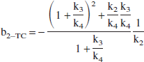
However, we have observed that the multilinear method applied to noisy data tends to yield positive results for both b and b′. Therefore, the operational Eq. 3 of the multilinear method was solved (least squares) with b and b′ constrained to negative values (b, b′≤0). A total of 10⁴ dynamic scans were simulated.

Parsey et al. (2000) performed [¹¹C](+)McN5652 PET in six healthy volunteers. Application of the invasive 1T-compartment model yielded k₂ = 0.009 ± 0.001 min⁻¹ and k′₂ = 0.014 ± 0.002 min⁻¹ in a receptor-rich region (thalamus) and a reference region (cerebellum), respectively (mean ± 1 SD). Using Eq. 18, this corresponds to b = −110 ± 10 minutes and b′ = −70 ± 10 minutes. Assuming that the values for each individual subject lie in the range mean ± 5 SD, one may formulate the physiologic constraints:

\begin{array}{l} R & \geq & 1 \\ b & \leq & - 60 min \\ b^{'} & \leq & - 20 min \end{array}

(20)

The operational Eq. 3 of the multilinear method was solved (least squares) using these constraints. A total of 10⁴ dynamic scans were simulated.

Regularization by Tikhonov-Phillips regularization with nonpositivity constraints

To evaluate the combined effect of filtered SVD and nonpositivity constraints, the operational Eq. 3 of the multilinear method was solved using Tikhonov-Phillips regularization with nonpositivity constraints imposed on b and b′ (Appendix). γ = 10 was chosen, and 10⁴ dynamic scans were simulated.

RESULTS

The results of the modeling are summarized in Table 1. Using the invasive 2T-compartment model (and Eqs. 4 and 6), the equilibrium DV ratio R was 2.07. This was the reference value. The multilinear method applied to the measured TACs, C_i and C′_i, yielded R = 1.44 (i.e., R was underestimated by about 30%). In addition, estimates for both b and b′ were positive, in contradiction to the compartment model interpretation. In contrast, application of the multilinear method to the model data, C͂_i and C͂′_i, reproduced the reference values of R, b, and b′ very accurately.

TABLE 1.

Results of modeling

Data	Model	Solution	R	b (min)	b′ (min)
Measured	2-tissue compartment model with arterial input	Nonlinear (Levenberg-Marquardt)	2.07	−71.8	−36.7
Measured	Multilinear	Least squares	1.44	9.1	12.3
Model, noise-free	Multilinear	Least squares	2.07	−72.4	−37.4
Model + noise (n = 10⁴)	Multilinear	Least squares	1.58 ± 0.07	−4.9 ± 6.5	1.8 ± 4.9
Model + noise (n = 10⁴)	Multilinear	Truncated SVD	1.57 ± 0.03	−4.3 ± 0.5	2.3 ± 0.3
Model + noise (n = 10⁴)	Multilinear	Tikhonov-Phillips	1.56 ± 0.03	−3.9 ± 0.6	2.0 ± 0.3
Model + noise, smoothed by cubic splines (n = 10⁴)	Multilinear	Least squares	1.64 ± 0.16	−12.9 ± 17.5	−2.9 ± 13.7
Model + noise (n = 10⁴)	Multilinear	Least squares + nonpositivity constraints	1.60 ± 0.05	−8.5 ± 2.9	−1.0 ± 1.8
Model + noise (n = 10⁴)	Multilinear	Least squares + physiologic constraints	1.98 ± 0.09	−60.0 ± 0.0	−31.7 ± 3.2
Model + noise (n = 10⁴)	Multilinear	Tikhonov-Phillips + nonpositivity constraints	1.56 ± 0.03	−6.1 ± 0.7	0

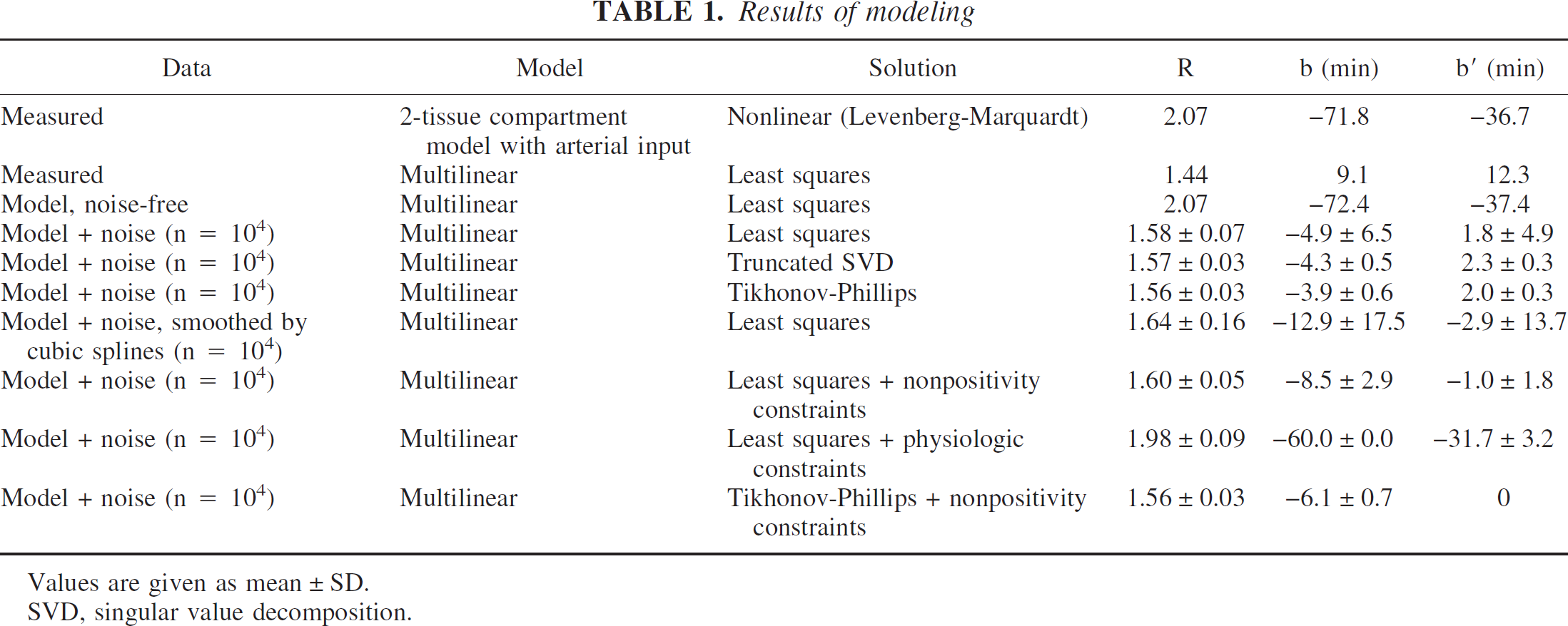
Values are given as mean ± SD.

SVD, singular value decomposition.

Application of the multilinear method to 10⁴ noisy data sets obtained from the model data by adding Gaussian noise yielded R = 1.58 ± 0.07 (mean ± 1 SD); that is, R was underestimated by almost 25%. With increasing noise (increasing ρ, Eq. 12), the mean value of R showed a slight decrease while the standard deviation increased (data not shown).

The singular values of the coefficient matrix Ã, computed from the model TACs C͂_i and C͂′_i, were σ₁ = 1.4 * 10⁵, σ₂ = 31, σ₃ = 0.5. Thus the condition number of Ã was very large, in the order of 10⁵. This implies instability of the multilinear method with respect to noise (Eq. A6). The left singular vectors of Ã are shown in Fig. 3 together with the left singular vectors of the coefficient matrix A, computed from the measured (noisy) TACs C_i and C′_i. The first two left singular vectors, u₁, u₂ corresponding to the singular values σ₁, σ₂ are very similar for the modeled Ã and the measured A. However, there is no similarity at all between the left singular vectors u₃ corresponding to the smallest singular value, σ₃, of Ã and A. The left singular vector u₃ of the measured coefficient matrix A is very noisy; it oscillates heavily around 0 (Fig. 3C). This causes the corresponding coefficient u^T₃y of the v₃-contribution to the least-squares solution of the multilinear method to be too small (Eq. A3). The components of v₃, the right singular vector to the smallest singular value σ₃, are shown in Fig. 4. The R-component of v₃ is positive, its (−R b′)-component is also positive, and its b-component is negative. This explains why underestimation of the coefficient u^T₃y, caused by oscillations of u₃ due to statistical noise, leads to systematic underestimation of R, and overestimation of both, b and b′.

FIG. 3.

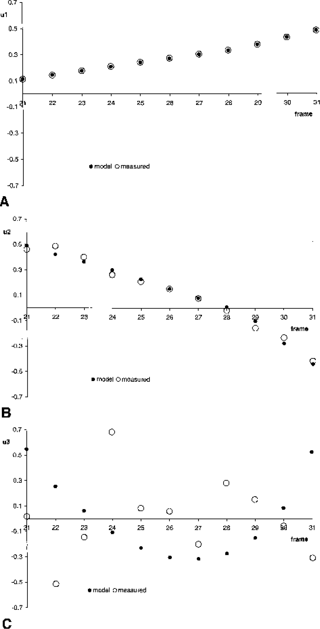
Singular value decomposition (SVD) of the coefficient matrix of the operational equation of the multilinear method: left singular vectors to the singular values σ₁ (A) > σ₂ (B) > σ₃ (C).

FIG. 4.

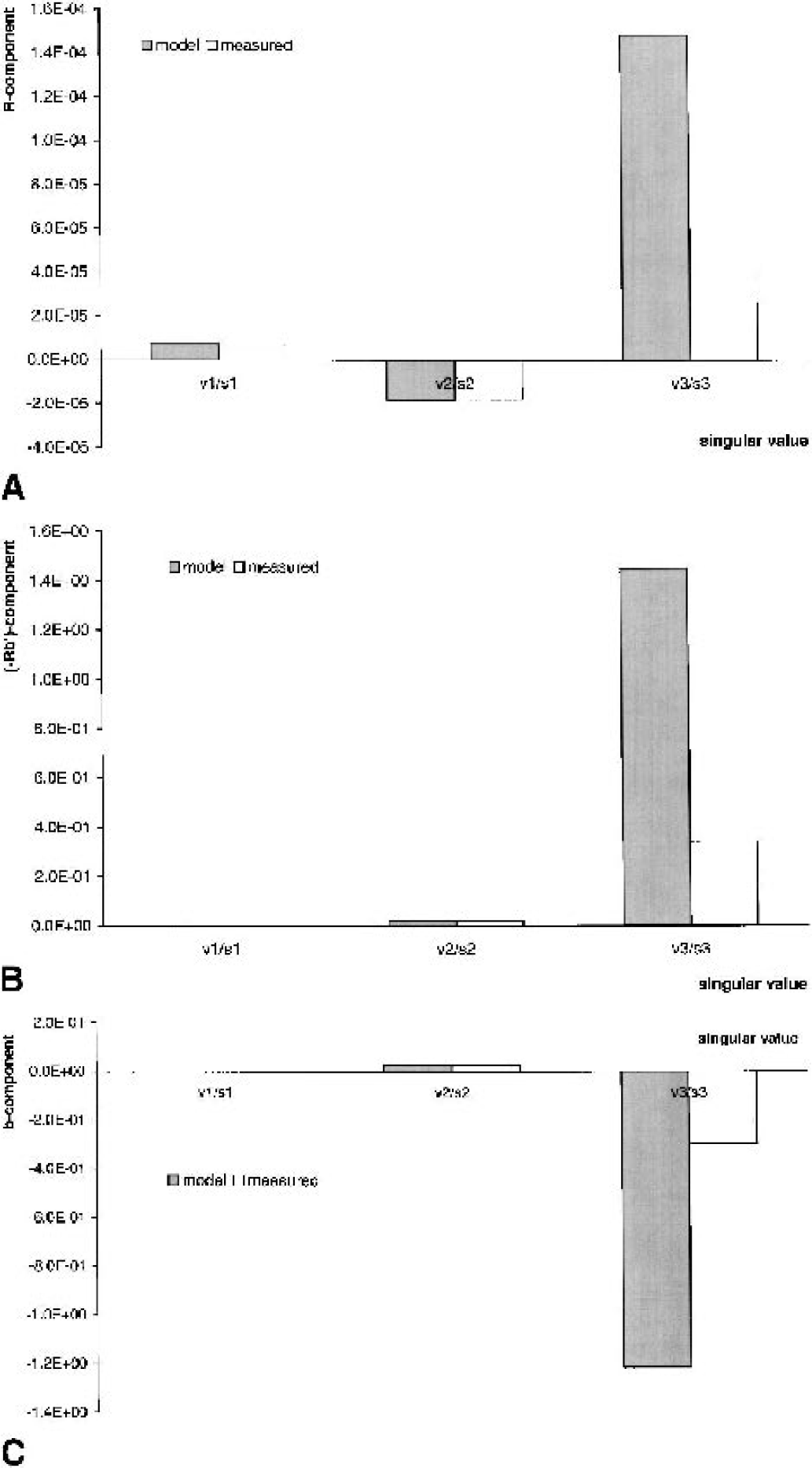
Singular value decomposition (SVD) of the coefficient matrix of the operational equation of the multilinear method: components of right singular vectors to the singular values σ₁ (A) > σ₂ (B) > σ₃ (C) divided by corresponding singular value (Eq. A3).

Since the contribution of u₃ to the solution of the multilinear method in case of noisy data was (almost) pure noise, it seemed reasonable to omit it. This is precisely the effect of TSVD with P = 2. As was to be expected, TSVD left mean values unchanged, but significantly reduced standard deviations. The standard deviation of R was reduced from 0.07 to 0.03 (i.e., by a factor of about 2).

Tikhonov-Philipps regularization (TP) yielded very similar results as TSVD. Nonpositivity constraints on b and b′ also provided stabilization, although somewhat less than TSVD and TP. The underestimation of R was slightly less severe than with TP and TSVD.

Application of physiologic constraints on b and b′ resulted in almost correct results for the DV ratios R. Underestimation of R was reduced to about 4%. The constraint on the parameter b (b≤–60 minutes = mean + 5 SD; Eq. 20) was consistently active (b = −60.0 ± 0.0 minutes; Table 1). Therefore, in order to analyze the sensitivity of R to the particular choice of the physiologic constraints, the upper bound of b was varied (keeping the upper bound of b′ fixed). This resulted in R = 2.28 ± 0.14 (b≤–100 minutes = mean + 1 SD), R = 2.13 ± 0.11 (b≤–80 minutes = mean + 3 SD), R = 1.98 ± 0.09 (b≤–60 minutes = mean + 5 SD), R = 1.84 ± 0.07 (b≤–40 minutes = mean + 7 SD), and R = 1.71 ± 0.06 (b≤–20 minutes = mean + 9 SD) (true value: R = 2.07). Thus, the estimates of R decreased with loosening the physiologic constraints and approached the value obtained with the nonpositivity constraints as the upper bound of b approached zero. However, the variation of the estimate of R was restricted to about ± 10% (relative to its value resulting when using b≤–60 minutes = mean + 5 SD) when the upper bound of b was varied between [mean + 1 SD] and [mean + 7 SD]. Moreover, the error (bias) of the estimate amounted to at most 10% for this range of constraints (error without regularization was approximately 25%).

The combination of TP and nonpositivity constraints did not provide further improvement, and the results obtained were almost the same as TSVD and TP without constraints.

DISCUSSION

The multilinear method applied to noisy TACs from a patient study underestimated the DV ratio R by about 30% as compared with quantification using the 2T-compartment model together with the arterial input function (kinetic modeling). However, application of the multilinear method to the model TACs, obtained from the full kinetic modeling, reproduced the reference value very accurately. This shows that the multilinear method is “correct,” in that it yields the correct result in a case of noiseless data.

In a second step the multilinear method was applied to 10⁴ noisy data sets obtained from the model data by adding Gaussian noise. R decreased with increasing noise levels. For realistic noise levels, R was underestimated by about 25%. This supports the hypothesis that the underestimation of R by the multilinear method is caused by its sensitivity with respect to statistical noise.

This finding was further confirmed by the SVD of the coefficient matrix of the operational equation of the multilinear method. The condition number was found to be extremely large, in that the multilinear method is rather ill conditioned (i.e., it is quite sensitive to statistical noise). In case of noisy data, the left singular vector corresponding to the smallest singular value was very noisy, its components oscillating heavily around zero. This caused a systematic underestimation of the contributions of the right singular vector corresponding to the smallest singular value. Since the contribution of this right singular vector to R was positive, this explained the systematic underestimation of R.

The multilinear method has been reported to provide increased test-retest reproducibility compared to invasive techniques (Acton et al., 2001). However, in order to further stabilize the algorithm by omission or suppression of the contributions of the smallest singular value, TSVD and the method of Tikhonov-Philipps was applied. Mean values of R were unchanged by these procedures, but the standard deviations were significantly reduced. Therefore, the test-retest stability of the multilinear method may be further improved by regularization. Taking into account that intersubject variability of the [¹¹C](+)McN5652 DV ratio obtained by the multilinear method is below 10% relative standard deviation (Buchert et al., 2003) the amount of the improvement of the test-retest stability by regularization is of practical relevance. It should be noted that improvement of test-retest stability is of practical relevance despite the fact that the error (bias) in the estimation of DV ratios is still large. Assuming that there is a stable one-to-one correspondence between the true values and the biased estimators, the power of a method to separate different groups of subjects (e.g., drug users versus drug naïves) or, in clinical applications, a single patient from a group of normal controls (e.g., by voxel-based analysis using SPM) strongly depends on the variance of the parameter of interest. In order to detect alterations of the receptor status, the examined parameter need not be unbiased. Thus, the ability to reduce the variance of a biased estimator is definitely desirable.

Imposing nonpositivity constraints on the rate constants provided stabilization, although somewhat less than TSVD or TP.

Simply smoothing noisy TACs before data evaluation resulted in even larger standard deviation of the DV ratio R as without smoothing and without regularization. This indicates that simple smoothing of TACs is not appropriate for the stabilization of the multilinear method because modeling itself is some kind of smoothing in time. Additional smoothing of TACs before modeling is redundant and should not be applied. Regularization cannot be achieved by simple smoothing.

The multilinear method yielded correct DV ratios when supplemented by linear boundary constraints on the combinations b and b′ of rate constants based on their normal range. The sensitivity of the estimate of R to the particular choice of the physiologic constraints was rather small over a wide range of constraints. Therefore, these constraints allow bias-free estimates of DV ratios. However, the formulation of physiologic constraints requires some knowledge about mean values and variances of rate constants in each population to be studied. Since the sensitivity of the method to the particular choice of the physiologic constraints is rather small, the physiologic constraints for normal volunteers used in the present paper should also be applicable to cases with mild pathology. In clinical applications with severe pathology, the formulation of physiologic constraints may be rather difficult so that the use of nonpositivity constraints might be preferred.

In the present paper, TACs of a single patient study were used to derive model data, to which simulated noise was added. However, the results presented here were confirmed by further simulation studies. TACs corresponding to different sets of rate constants were generated using the invasive 1T-compartment model and a simulated arterial input function after a bolus injection of 400 MBq [¹¹C](+)McN5652 (data not shown).

The Logan plot is also known to introduce a bias that results in the underestimation of distribution volumes (DVs) (Carson, 1993). The bias depends not only on the level of statistical noise but also on the magnitude of the DV, and it is more pronounced at high level of statistical noise and at large DV (Slifstein and Laruelle, 2000). The underestimation of DVs by the Logan plot is related to the fact that simple linear regression takes into account errors in the y variable but not errors in the × variable (Slifstein and Laruelle, 2000). The regularization methods discussed here account for errors on both sides of the operational equation (Appendix). However, regularization alone could not avoid the underestimation of the DV ratio.

Different strategies have been described to avoid the underestimation of DVs by the Logan plot. Logan et al. (2001) proposed a modification of the generalized linear least squares method developed by Feng et al. (1993), which essentially is an iterative approach to the solution of the operational equation. Varga and Szabo (2002) applied a linear regression model that minimizes the sum of squared perpendicular rather than vertical distances between data points and the fitted straight line. This regression model accounts for errors in both the × and y variables of the straight line. Recently, Ichise et al. (2002) reported attempts to improve neuroreceptor DV estimates based on mathematical rearrangement of the operational equation. The main drawbacks of these techniques are that the compensation is only partial, and they result in increased test-retest variability. Therefore, it might be useful to combine these methods with the regularization procedures that we have described here.

CONCLUSIONS

Underestimation of equilibrium DV ratios by the multilinear method is caused by its sensitivity to statistical noise. The bias can be reduced by imposing boundary constraints. Regularization procedures do significantly improve the stability of the multilinear method, which results in increased statistical power.

Footnotes

APPENDIX

References

Computational Science Education Project (1995) Error bounds for solving Ax = b. Numerical Linear Algebra. Available at: http://csep1.phy.ornl.gov/csep.html

Acton

Choi

Hou

Plossl

Kung

(2001) Quantification of serotonin transporters in nonhuman primates using [(123)I]ADAM and SPECT. J Nucl Med 42:1556–1562

Buchert

Thomasius

Nebeling

Petersen

Obrocki

Jenicke

Wilke

Wartberg

Zapletalova

Clausen

(2003) Long-term effects of “ecstasy” use on serotonin transporters of the brain investigated by positron emission tomography. J Nucl Med 44:375–384

Buck

Gucker

Schonbachler

Arigoni

Kneifel

Vollenweider

Ametamey

Burger

(2000) Evaluation of serotonergic transporters using PET and [¹¹C](+)McN-5652: assessment of methods. J Cereb Blood Flow Metab 20:253–262

Carson

(1993) PET parameter estimation using linear integration methods: bias and variability. Quantification of brain function: tracer kinetic and image analysis in brain PET ( Uemura

Lassen

Jones

Kanno

, eds), New York: Excerpta Medica, pp 499–507

De Boor

(1987) A practical guide to splines. New York, Springer

Feng

Wang

Huang

S-C

(1993) A study on statistically reliable and computationally efficient algorithms for the measurement of local cerebral blood flow with positron emission tomography. IEEE Trans Med Imag 12:182–188

Hansen

(1994) Regularization tools: a MATLAB package for analysis and solution of discrete ill-posed problems. Numerical Algorithms 6:1–35

Hansen

(1998) Rank-deficient and discrete ill-posed problems. Philadelphia: SIAM Society for Industrial and Applied Mathematics

10.

Ichise

Ballinger

Golan

Vines

Luong

Tsai

Kung

(1996) Noninvasive quantification of dopamine D₂ receptors with iodine-123-IBF SPECT. J Nucl Med 37:513–520

11.

Ichise

Meyer

Yonekura

(2001) An introduction to PET and SPECT neuroreceptor quantification models. J Nucl Med 42:755–763

12.

Ichise

Toyama

Innis

R B

Carson

R E

(2002) Strategies to improve neuroreceptor parameter estimation by linear regression analysis. J Cereb Blood Flow Metab 22:1271–1281

13.

Laruelle

Wallace

Seibyl

Baldwin

Zea-Ponce

Zoghbi

Neumeyer

Charney

Hoffer

Innis

(1994) Graphical, kinetic, and equilibrium analyses of in vivo [¹²³I] β-CIT binding to dopamine transporters in healthy human subjects. J Cereb Blood Flow Metab 14:982–994

14.

Logan

(2000) Graphical analysis of PET data applied to reversible and irreversible tracers. Nucl Med Biol 27:661–670

15.

Logan

Fowler

Volkow

Ding

Wang

Alexoff

(2001) A strategy for removing the bias in the graphical analysis method. J Cereb Blood Flow Metab 21:307–320

16.

Logan

Fowler

Volkow

Wolf

Dewey

Schlyer

Macgregor

Hitzemann

Bendriem

Gatley

(1990) Graphical analysis of reversible radioligand binding from time-activity measurements applied to[n-¹¹C-methyl]-(−)-cocaine PET studies in human subjects. J Cereb Blood Flow Metab 10:740–747

17.

Louis

(1989) Inverse und schlecht gestellte probleme. Stuttgart, B.G. Teubner

18.

McCann

Szabo

Scheffel

Dannals

Ricaurte

(1998) Positron emission tomographic evidence of toxic effect of MDMA (“ecstasy”) on brain serotonin neurons in human beings. Lancet 352:1433–1437

19.

Meyer

Wilson

Ginovart

Sagrati

Carella

Houle

(2002) Dose occupancy relationship of five selective serotonin reuptake inhibitors using [¹¹C] DASB PET. London: NeurReceptor Mapping 2002. Available at: http://www.academicpress.com/www/journal/nrm2002/14025.html

20.

Meyer

Wilson

Ginovart

Goulding

Hussey

Hood

Houle

(2001) Occupancy of serotonin transporters by paroxetine and citalopram during treatment of depression: a [(11)C]DASB PET imaging study. Am J Psychiatry 158:1843–1849

21.

Mikolajczyk

Szabatin

Rudnicki

Grodzki

Burger

(1998) A JAVA environment for medical image data analysis: initial application for brain PET quantitation. Med Inform (Lond) 23: 207–214

22.

Parsey

Kegeles

Hwang

Simpson

Abi-Dargham

Mawlawi

Slifstein

Van Heertum

Mann

Laruelle

(2000) In vivo quantification of brain serotonin transporters in humans using [¹¹C]McN5652. J Nucl Med 41:1465–1477

23.

Patlak

Blasberg

Fenstermacher

(1983) Graphical evaluation of blood-to-brain transfer constants from multiple-time uptake data. J Cereb Blood Flow Metab 3:1–7

24.

Slifstein

Laruelle

(2000) Effects of statistical noise on graphic analysis of PET neuroreceptor studies. J Nucl Med 41:2083–2088

25.

Suehiro

Scheffel

Dannals

Ravert

Ricaurte

Wagner

Jr (1993) A PET radiotracer for studying serotonin uptake sites: carbon-11-McN-5652Z. J Nucl Med 34:120–127

26.

Szabo

Kao

Scheffel

(1995) Positron emission tomography imaging of serotonin transporters in the human brain using [¹¹C](+)McN5652. Synapse 20:37–43

27.

Szabo

Scheffel

Mathews

Ravert

Szabo

Kraut

Palmon

Ricaurte

Dannals

(1999) Kinetic analysis of [¹¹C]McN5652: a serotonin transporter radioligand. J Cereb Blood Flow Metab 19:967–981

28.

Varga

Szabo

(2002) Modified regression model for the Logan plot. J Cereb Blood Flow Metab 22:240–244

Improved Statistical Power of the Multilinear Reference Tissue Approach to the Quantification of Neuroreceptor Ligand Binding by Regularization*

Abstract

Keywords

MATERIALS AND METHODS

Multilinear method

Data

Statistical noise

Singular value decomposition

Regularization by truncated singular value decomposition

Regularization by Tikhonov-Phillips regularization

Smoothing of time–activity curves

Constraints

Regularization by Tikhonov-Phillips regularization with nonpositivity constraints

RESULTS

DISCUSSION

CONCLUSIONS

Footnotes

APPENDIX

References