Sage Journals: Discover world-class research

Abstract

Variable selection methods play an important role in high-dimensional statistical modeling and analysis. Computational cost and estimation accuracy are the two main concerns for statistical inference from ultrahigh-dimensional data. In particular, genome-wide association studies (GWAS), which focus on identifying single nucleotide polymorphisms (SNPs) associated with a disease of interest, have produced ultrahigh-dimensional data. Numerous methods have been proposed to handle GWAS data. Most statistical methods have adopted a two-stage approach: pre-screening for dimensional reduction and variable selection to identify causal SNPs. The pre-screening step selects SNPs in terms of their P-values or the absolute values of the regression coefficients in single SNP analysis. Penalized regressions, such as the ridge, lasso, adaptive lasso, and elastic-net regressions, are commonly used for the variable selection step. In this paper, we investigate which combination of pre-screening method and penalized regression performs best on a quantitative phenotype using two real GWAS datasets.

Keywords

genome-wide association study the Korea Association Resource (KARE)the Age-Related Eye Disease Study (AREDS)penalized regression variable selection

Introduction

Recently, many high-dimensional datasets have been generated in biomedical science, such as microarrays and single nucleotide polymorphism (SNP) databases. In particular, genome-wide association studies (GWAS), which focus on identifying SNPs associated with a disease of interest, have produced ultrahigh-dimensional data. For theoretical development, we consider data to have high dimensionality if p = O(n^a) for some a≫0, and to have ultra-high dimensionality if log p = O(n^a) for some a≫0. When the dimension p is high, we run into the often-fatal “curse of dimensionality.” The convergence of any estimator to the true value of a smooth function defined on a space of high dimension is very slow. Variable selection plays an important role in high-dimensional statistical modeling and analysis. Computational cost and estimation accuracy are the two main concerns for statistical inference from high-dimensional data.

Many efficient approaches have been introduced to overcome these problems. One is the adoption of multistep strategies.^1,2 The first stage of this approach reduces the dimensionality P for significant predictor selection in ultrahigh-dimensional data. This pre-screening stage is used to find variables that may only be marginally associated with a response variable. This step reduces the dimension of the dataset and makes joint analysis possible. Therefore, the multistep approach indicates one solution for the ultrahigh-dimensional problem. Several predictor selection tools have been developed to implement the above idea for ultrahigh-dimensional linear models. Sure independence screening (SIS), which is the most widely used pre-screening method,^3,4 ranks the predictor variables using the absolute values of the correlation coefficients as a criterion. Another pre-screening method is described in Cho et al.¹, which uses the pre-screening step to identify marginally associated responses, using the P-value as a criterion.

We want to know which of the available pre-screening methods is better for quantitative traits. Although many pre-screening methods are available, we do not know which method performs best in predicting a particular quantitative phenotype. We can find predictors that are jointly associated with the response variable among the parameters that remain after the pre-screening step. When multiple predictor variables exist for a response variable, joint identification becomes a powerful tool.¹

One of the traditional approaches for joint identification is the multiple linear/logistic regression method. However, when we handle high-dimensional data using traditional methods, we experience several problems. First, multiple linear regressions do not work well within high dimensionality, which causes computational complexity. Second, multiple linear regression is very sensitive to multicollinearity among SNPs. To overcome this problem, various penalization methods have been proposed, such as the ridge, bridge, least absolute shrinkage and selection operator (lasso), adaptive lasso, smoothly clipped absolute deviation (SCAD), and elastic-net.^5–9 These methods can find jointly associated variables in high-dimensional data. The elastic-net method uses both the ridge and lasso penalties, obtaining the advantages of both approaches. The elastic-net method automatically selects significant variables, and, thus, efficiently resolves the problem caused by multicollinearity. The iterative adaptive lasso (IAL) method¹⁰ retains the appealing property of rapid computation even for ultrahigh-dimensional problems. This method yields a sparse solution by setting certain parameters to zero. Predictor selection is then achieved with the nonzero values.

Many methods have been suggested for pre-screening and the variable selection procedure. However, we do not know which method performs best for quantitative traits. In this paper, we investigate which combination of pre-screening method and penalized regression performs best. To compare the power of pre-screening methods and penalized regressions, we use two GWAS datasets: one from the Korea Association Resource (KARE) project and the other from the Age-Related Eye Disease Study (AREDS). The adjusted R-square is used as a measure of comparison.¹¹

Materials and Methods

Materials

KARE Data

The KARE project began in 2007.¹¹ Participants in this project were recruited from two community-based cohorts: the rural Ansung cohort and the urban Ansan cohort in Gyeonggi-do province of South Korea. The numbers of people in the Ansung and Ansan cohorts are 5,018 and 5,020, respectively. The age range is from 40 to 69 years. More than 260 phenotypes have been surveyed through physical examinations, epidemiological surveys, and laboratory tests. We focus on the height trait, because height is a highly heritable polygenic characteristic.¹¹

The KARE data contain 500,568 SNPs. Before analysis, quality control processes are performed following Cho et al.¹, and missing genotypes are imputed using PLINK software and the Japanese in Tokyo (JPT)/Han Chinese in Beijing (CHB) reference panel in HapMap.¹ After these processes, we obtain a dataset with 327,872 SNPs from 8,842 individuals.

Areds Data

AREDS is a prospective study of 4,757 persons to establish the risk factors of both age-related macular degeneration (AMD) and cataract.¹² The AREDS began in 1992. Ages of participants ranged from 55 to 80 years. Participants have been followed for at least seven years. We used body mass index (BMI) as a quantitative trait. The genotype platform of the AREDS data is an Illumina 100K GWAS chip. A total of 525 individuals were genotyped. Quality control processes were performed using the same criteria as with the KARE data. After quality control, we obtained a dataset with 87,260 SNPs from 462 individuals.

Methods

We formulate a multistage strategy for identifying the significant parameters among an enormous number of explanatory variables. Our strategy consists of three stages. At stage 1, we screen out the variables that are weakly correlated with the response variable via single-variable association tests. We select variables in terms of their P-values or by the absolute values of their regression coefficients in single-variable analysis. At stage 2, we search for multiple-variable associations by using penalized multiple regression with the elastic-net, ridge, lasso, and IAL methods. At stage 3, using the elastic-net and lasso methods, we assess the jointly identified variables using bootstrap selection stability (BSS), which is proposed empirically to assess with what consistency a variable is selected from the bootstrap samples.¹ Using the ridge and IAL methods, we assess the jointly identified variables by using the effect size.

Stage 1. Standardization

Suppose that y_i for i = 1, n are the responses for the ith individual, and x_ij for j = 1, …, p are its predictors. We assume that the predictors are standardized to have zero mean and unit standard deviation in order to maintain generality.

E (x_{i j}) = 0 and E (x_{i j}^{2}) = 1 for i = 1, …, n; j = 1, …, p .

Stage 2. Pre-screening

We use the linear regression model in order to eliminate predictors that are weakly correlated with the response variable to achieve dimensionality reduction.

y_{i} = γ_{o} + \sum_{q = 1}^{Q} γ_{q} z_{i q} + β_{j} x_{i j} + ε_{i},

where z_q represents the adjustment variables for the ith case. All variables are ranked in ascending order of P-values or in descending order of absolute value of coefficients from single-variable analysis. According to the order, the top P variables showing the strongest marginal associations with the response variables are selected.

Stage 3. Variable selection

Method 1

Penalized regression. Multiple linear models are fitted for the selected top P variables after adjusting for the covariates.

y_{i} = γ_{o} + \sum_{q = 1}^{Q} γ_{q} z_{i q} + \sum_{j = 1}^{P} β_{j} x_{i j} + ε_{i}

We find the optimal solution by using penalized regressions such as the ridge, lasso, and elastic-net. The penalized regressions find the solution as follows:

\begin{matrix} \hat{β} = \underset{(β, γ)}{\arg \min} [- L (β, γ) + λ P_{α} (β)], \\ where p_{α} (β) = \frac{1}{2} (1 - α) | | β | |_{l_{2}}^{2} + α | | β | |_{l_{1}} \\ = \sum_{j = 1}^{P} [\frac{1}{2} (1 - α) β_{j}^{2} + α | β_{j} |] . \end{matrix}

The amount of shrinkage is represented by parameter λ. We can find an optimal λ by using tenfold cross-validation, which accomplishes mean squared error minimization. Ridge regression (α = 0) entails a shrinkage of the least squares estimators.⁸ The ridge is a biased estimator. Since the ridge reduces the variance of the estimators, it reduces the mean square error. In cases of high dimensionality, the ridge provides a shrinkage factor that does not accomplish variable selection. The lasso (α = 1) has an l₁-norm penalty function.⁵ Thus, the lasso produces coefficients of zero for insignificant variables. The lasso thus automatically performs variable selection. The elastic net method includes the lasso and ridge regressions. In other words, each of them is a special case where α = 1 or α = 0. The elastic net thus has the advantages of both the ridge and lasso regularizations. Variables showing strong joint association with the response variable are automatically selected via the elastic net method. Therefore, the elastic net has the ability to perform grouped selection of highly correlated variables.

Method 2. IAL

The IAL method is a two-stage procedure.¹⁰ At the first stage, single-variable analysis is implemented to rank the magnitude of the marginal linear regression estimators. At the second stage, a weighted least-squares-type objective function is used to approximate a potential function. This allows us to further define a penalized weighted least square (PWLS) model for moderate-scale selection.

Step 1. Let M = {j | β_j ≫ 0, j = 1,…, p}. We need first to predetermine a sparsity parameter size d. It is recommended to take d = n/(logn). For each variable, the single-variable association with phenotype is examined using linear regression. The jth predictor is ${\hat{β}}_{j}^{^{M}}$ . The predictors are ranked in descending order of values. From the first predictor to the k₁ th are considered as the set A₁, where k₁ = [2d/3]. This value of k₁ is recommended in order to guarantee at least two iterations. Variables of set A₁ fit joint linear regression. The predictor is ${\hat{β}}_{j}^{^{M}}$ . We then employ the PWLS procedure:

\begin{array}{l} \hat{β} = \arg \min [- L (β, γ) + λ P (β)], \\ P (β) = \sum_{j = 1}^{p} w_{j} | β_{j} | w h e r e w_{j} = | {\hat{β}}_{j}^{M} | - 1 \end{array}

to select a subset M₁ of A₁.

Step 2. For every j ∊ M₁^c = [1,….., p}\M₁. estimate ${\hat{β}}_{j}$ as follows:

y_{i} = β_{0} + \sum_{i = l}^{n} (X_{i (M_{1})}) β^{M_{1}} + X_{i j} β_{j}) + ε_{i} .

After ordering ${| {\hat{β}}_{j} | : j \in M_{1}^{C}}$ , pick up a set A₂ of indices of size k₂ = d - |M₁|.

Step 3. Apply the PWLS procedure at {M₁, A₂}. The nonzero elements of the variable yield a new significant index M₂.

Step 4. Iterate steps 2–3 until |M_l|≥ d or | M_l |=| M_l-1|.

Step 5. Finally, we obtain both the predictor set $\hat{M}$ and the estimated parameter vector. The magnitudes of the absolute values of the marginal linear regression estimators can preserve the nonsparse information of the joint regression model. This procedure contains the sure screening property.³ This large-scale screening method can be regarded as an extension of the SIS procedure.⁴ It retains the appealing property that it can be rapidly computed even for ultrahigh-dimensional problems. PWLS yields a sparse solution by setting some parameters to zero. Thereafter, predictor selection is achieved with the nonzero values. The adaptive lasso method can also reduce bias.

Stage 4. Ordering

After selecting the significant predictor variables, we rank them in order of importance. For the elastic-net and lasso methods, we use BSS. Joint selection of SNPs via the elastic-net method is performed for the bootstrap samples. Bootstrapping is a resampling technique: a bootstrapping sample is a random sample with replacements from the original dataset. The bootstrap sample size is equal to the original dataset size. B bootstrap samples are generated. BSS is defined for the ith variables as follows.

\begin{array}{l} {BSS}_{i} = \frac{1}{B} \sum_{b = 1}^{B} I_{i}^{b}, \\ where I_{i}^{b} = {\begin{array}{l} 1 if replicated in the b th bootstrap sample \\ 0 otherwise \end{array} \end{array}

BSS signifies how many times each selected predictor variable is replicated in B bootstrap datasets. SNPs are ranked in descending order of BSS.

For the ridge and IAL methods, the selected significant predictor variables are ranked in descending order of effect size.

Results

Pre-screening

KARE Data

At this step, we use the linear regression model in order to perform single SNP analysis for 327,872 SNPs. This linear regression model includes adjustment variables such as gender, age, and recruitment area (rural Ansung and urban Ansan).

{height}_{i} = γ_{0} + γ_{1} {SEX}_{i} + γ_{2} {AGE}_{i} + γ_{3} {AREA}_{i} + β_{j} {SNP}_{i j} + ε_{i},

where i = 1, 2, …, 8,842 denotes the individuals and j = 1, 2, …, 327,872 represents the SNPs. All SNPs are ranked in ascending order of P-values or in descending order of the absolute values of the coefficients from single-variable analysis. We use the top 1,000 ranked SNPs for each criterion, namely, the P-values and the absolute values of coefficients. We compare the minor allele frequency (MAF) and the number of missing values of the selected SNPs for each criterion. For the P-value criterion, the number of rare variants whose MAF values are less than 0.05 is 87. For the absolute values of coefficients criterion, the number of rare variants is 991 (Fig. 1). We observe that the common variants tend to have large numbers of missing values.

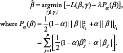
Although we use imputation processes, there are still missing values. Therefore, individuals having at least one missing value are eliminated. When data include individuals who have at least one missing value, penalized regressions such as the elastic-net and adaptive lasso cannot be performed. After the elimination process is performed, the number of remaining individuals is 4,183 for the P-value criterion and 7,496 for the absolute values of coefficients criterion. The number of overlapping individuals is 3,740. We use these overlapping individuals to compare each combination method. However, too many individuals have been lost. In order to reduce the loss of data, we eliminated SNPs with more than 30 missing values. The number of remaining SNPs is then 944 for the P-value criterion and 984 for the absolute values of coefficients criterion. After the elimination process, the remaining number of individuals is 7,481 for the P-value criterion and 8,164 for the absolute values of coefficients criterion. The number of overlapping individuals is 7,061. Henceforth, we shall use these individuals.

Areds Data

For the AREDS data, we use the linear regression model in order to perform single SNP analysis for 87,260 SNPs on the AREDs data. The model is given as follows:

{bmi}_{i} = γ_{0} + γ_{1} {SEX}_{i} + β_{j} {SNP}_{i j} + ε_{i},

where i = 1, 2, …, 461 are the individuals and j = 1, 2, …, 87,260 are the SNPs. All SNPs are ranked in ascending order of P-values or in descending order of the absolute values of the coefficients from single-variable analysis. We use the top 1,000 ranked SNPs via the P-values and absolute values of coefficients.

Figure 1

Number of missing data in the top 1,000 variables for each filtering method. The X-axis shows the MAFs of each SNP and the Y-axis shows the number of missing data for each SNP. The left figure shows the case where the SNPs are filtered out by P-values. In this case, the MAFs of the SNPs are uniformly distributed. The right figure shows the case where the SNPs are filtered by the absolute values of coefficients. In this case, mainly rare variants are chosen.

Table 1.

Top 10 SNPs in each method after coefficient filtering of KARE data by effect size for each method.

RS NUMBER	CHR	POS	ALLELE1	ALLELE2	GENE	INCLUDED IN TOP 10	REPORTED
rs41338750	4	6346712	A	G	PPP2R2C	Lasso, elastic-net
rs344584	19	6604018	G	C		Lasso, elastic-net
rs7460090	8	57194163	T	C		Lasso, elastic-net
rs17535067	1	108074954	G	A		Lasso, elastic-net
rs17328296	5	93956986	A	G	ANKRD32	Lasso
rs10979023	9	110477887	G	A		Lasso, elastic-net
rs3755652	3	27472936	C	T	SLC4A7	Lasso, ridge
rs792965	5	172275263	G	A	ERGIC1	Lasso
rs953759	13	88484867	T	A		Lasso
rs330972	11	39170787	A	G		Lasso
rs10948187	6	44921320	C	T	SUPT3H	Elastic-net	*
rs3799977	6	44837356	T	G	SUPT3H	Elastic-net	*
rs2643626	12	56726518	G	A	PAN2	Elastic-net, ridge
rs12663931	6	82301126	T	C		Elastic-net
rs2292239	12	56482180	T	G	ERBB3	Elastic-net
rs7773193	6	28611334	C	T		IAL
rs7954185	12	94096173	A	T	CRADD	IAL	*
rs7969076	12	94096042	T	C	CRADD	IAL	*
rs13078798	3	27445971	G	A	SLC4 A7	IAL
rs2394119	6	28627517	T	A		IAL
rs7761914	6	28642509	G	A		IAL
rs6456829	6	28654152	C	G		IAL, ridge
rs1440744	8	57457322	G	C	LINC00968	IAL, ridge
rs4871557	8	125871112	T	C		IAL
rs4412192	6	26290377	G	A		IAL
rs206313	3	162491873	G	A		Ridge
rs2610021	8	57479553	G	C		Ridge
rs7674423	4	6312004	G	T		Ridge
rs11171806	12	56733531	G	A	STAT2	Ridge
rs9262494	6	30986504	C	T	MUC22	Ridge
rs6925972	6	28601934	A	T		Ridge

Variable Selection

KARE Data

We fit the multiple linear regression model to select the top 944 jointly associated SNPs for the 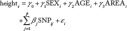P-value criterion and the top 984 SNPs for the absolute values of coefficients criterion.

\begin{matrix} {height}_{i} = γ_{0} + γ_{1} {SEX}_{i} + γ_{2} {AGE}_{i} + γ_{3} {AREA}_{i} \\ + \sum_{j = 1}^{P} β_{j} {SNP}_{i j} + ε_{i} \end{matrix}

All tuning parameters are determined by 10-fold cross-validation, which minimizes the mean squared error.

We can make eight combinations: (P-value + elastic-net), (P-value + lasso), (P-value + ridge), (P-value + IAL), (absolute values of coefficients + elastic-net), (absolute values of coefficients + lasso), (absolute values of coefficients + ridge), and (absolute values of coefficients + IAL). The combination method identifies 524, 504, 944, 471, 549, 548, 984, and 530 SNPs for these eight combinations, respectively, as putative height-related genetic variants. Then, for the elastic regularization and lasso methods, we generate 1,000 bootstrapped sets. The same fixed value of λ is used for the generated bootstrapped datasets. We can then determine the BSS value of each SNP. The SNPs are ranked in descending order of BSS. The ridge method cannot perform variable selection, as it selects all the SNPs. Therefore, BSS is meaningless in the ridge approach. For the ridge and adaptive lasso methods, the SNPs are ranked in descending order of effect size.

Table 2.

Top 10 SNPs in each method after P-value filtering of KARE data.

RS NUMBER	CHR	POS	ALLELE1	ALLELE2	GENE	INCLUDED IN TOP 10
rs17530546	2	42000661	T	C		Lasso, elastic-net
rs540270	13	27112888	C	T		Lasso, elastic-net
rs17527383	18	10085363	C	T		Lasso, elastic-net
rs8061362	16	68008679	G	A	DPEP3	Lasso, elastic-net
rs1322545	9	101642931	A	G		Lasso, elastic-net
rs10493974	1	102296144	T	G	OLFM3	Lasso, elastic-net
rs41338750	4	6346712	A	G	PPP2R2C	Lasso, elastic-net
rs2143795	6	103810408	C	T		Lasso, elastic-net
rs11890449	2	234199401	C	T	SCARNA6	Lasso, elastic-net
rs11089728	22	35492313	C	T		Lasso
rs2359104	1	34982227	G	T		Elastic-net, ridge
rs34422081	4	101942847	T	C	PPP3CA	IAL, ridge
rs41498549	4	101942806	T	C	PPP3CA	IAL
rs7658531	4	6312175	T	C		IAL
rs17328637	5	93959165	G	A	ANKRD32	IAL
rs7676014	4	6312079	C	G		IAL
rs4394651	1	159534446	C	G		IAL, ridge
rs4458523	4	6289986	T	G	WFS1	IAL
rs2808636	1	159566647	C	T		IAL, ridge
rs1890207	20	22514828	T	G		IAL, ridge
rs1046314	4	6303955	G	A	WFS1	IAL
rs6786503	3	73793932	T	A		Ridge
rs9314935	13	29685729	A	G	MTUS2	Ridge
rs1890207	20	22514828	T	G		Ridge
rs4394651	1	159534446	C	G		Ridge
rs9291619	4	14008860	G	A		Ridge
rs2808636	1	159566647	C	T		Ridge
rs2359104	1	34982227	G	T		Ridge
rs7981556	13	29692759	T	C	MTUS2	Ridge
rs199757	6	25981648	A	G	TRIM38	Ridge

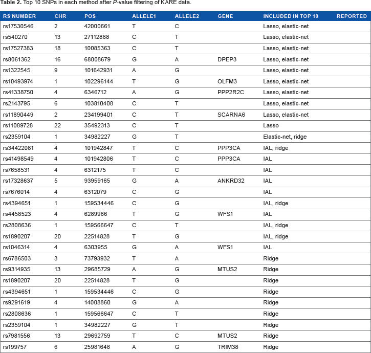
Table 1 shows the results of filtering SNPs with absolute value of coefficients in single variant analysis. Table 1 summarizes the list of SNPs that have the top 10 absolute values of coefficients in each penalized method. Among these SNPs, rs10948187, rs3799977, rs7954185, and rs7969076 were reported in other studies.^13,14 Table 2 shows the results of filtering SNPs with P-values in single variant analysis. It summarizes the list of SNPs that have the top 10 absolute values of coefficients in each penalized method.

AREDS data.

We fit the multiple linear regression model to select the top 1,000 jointly associated SNPs for the P-value criterion and the top 1,000 SNPs for the absolute values of coefficients criterion.

{bmi}_{i} = γ_{0} + γ_{1} {SEX}_{i} + \sum_{j = 1}^{P} β_{j} {SNP}_{i j} + ε_{i}

All tuning parameters are determined by 10-fold cross-validation, which minimizes the mean squared error. The combination method identifies 493, 460, 1000, 559, 485, 442, 1000, and 534 SNPs for the eight combinations, respectively, as putative BMI-related genetic variants.

Table 3.

Top 10 SNPs in each method after coefficient filtering of AREDS data.

RS NUMBER	CHR	POS	ALLELE1	ALLELE2	GENE	INCLUDED IN TOP 10
rs214531	6	18290122	T	A		Lasso, elastic-net, IAL, ridge
rs10501623	11	86291625	T	G	ME3	Lasso, elastic-net
rs10513842	3	189552478	C	G	TP63	Lasso, elastic-net, IAL, ridge
rs10499156	6	129688123	G	A	LAMA2	Lasso, elastic-net, IAL, ridge
rs9291876	5	66471420	T	A		Lasso, elastic-net, IAL, ridge
rs1040535	6	22647683	G	A		Lasso
rs10487745	7	122634409	G	T	TAS2R16	Lasso, elastic-net, IAL
rs10499520	7	21031746	T	C		Lasso, elastic-net
rs2341825	7	132094453	C	A	PLXNA4	Lasso, elastic-net
rs10519877	4	148122660	G	A		Lasso
rs10516605	4	115797475	T	C	NDST4	Elastic-net, IAL
rs1428186	5	38209532	C	A		Elastic-net, IAL
rs10501623	11	86291625	T	G	ME3	IAL
rs7916322	10	64612824	G	A		IAL
rs952930	1	74183266	A	G		IAL
rs982067	4	19364716	C	G		Ridge
rs10507076	12	97043549	T	C		Ridge
rs7653030	3	8873953	G	A		Ridge
rs10495828	2	34955423	T	C		Ridge
rs12081	15	40618613	G	C		Ridge
rs9297091	6	18767825	C	T		Ridge

Table 4.

Top 10 SNPs in each method after P-value filtering of AREDS data.

RS NUMBER	CHR	POS	ALLELE1	ALLELE2	GENE	INCLUDED IN TOP 10
rs10493273	chr1	60430348	T	C		Lasso, elastic-net, IAL, ridge
rs10493424	chr1	67957208	G	C		Lasso, elastic-net, IAL
rs1407508	chr9	101644538	T	C		Lasso, elastic-net, IAL, ridge
rs2364922	chr2	84539921	G	T		Lasso, elastic-net, IAL
rs10509345	chr10	75361303	T	C		Lasso, elastic-net
rs10497376	chr2	172495027	T	C		Lasso, elastic-net, IAL
rs10499171	chr6	130302794	C	A		Lasso, elastic-net, IAL
rs7024617	chr9	102139440	C	T	NAMA	Lasso, elastic-net, IAL, ridge
rs9288172	chr2	191250278	T	C		Lasso, elastic-net
rs10486965	chr7	82150331	A	G		Lasso, elastic-net
rs7791296	chr7	54220890	G	T		IAL
rs7179842	chr15	88135030	A	G		IAL
rs10499171	chr6	130302794	C	A		IAL
rs10506150	chr12	40666760	A	T	LRRK2	IAL
rs982067	chr4	19364716	C	G		Ridge
rs10507076	chr12	97043549	T	C		Ridge
rs7653030	chr3	8873953	G	A		Ridge
rs12081	chr15	40618613	G	C		Ridge
rs1922128	chr10	53347934	A	G	PRKG1	Ridge
rs10496550	chr2	119349987	A	G		Ridge
rs10499520	chr7	21031746	T	C		Ridge

Table 3 shows the results of filtering SNPs with absolute values of coefficients in single variant analysis. Table 3 summarizes the list of SNPs that have the top 10 absolute values of coefficients in each penalized method. Table 4 shows the results of filtering SNPs with P-values in single variant analysis. It summarizes the list of SNPs that have the top 10 absolute values of coefficients in each penalized method.

Comparative Study

We calculated the adjusted R-squares for the selected SNPs to investigate which combination of pre-screening method and penalized regression performs best for predicting quantitative traits. SNPs are ranked by BSS for the elastic-net and the lasso methods, while SNPs are ranked by effect size for the IAL and ridge methods.

Figure 2

Comparison of adjusted R-squares when the SNPs are filtered out by P-values in KARE data analysis. The X-axis represents the number of SNPs and the Y-axis the adjusted R-squares. The SNPs are ranked by BSS for the elastic-net and lasso methods, while the SNPs are ranked by effect size for the IAL and ridge methods.

Figure 3

Comparison of adjusted R-squares when SNPs are filtered out by effect size in KARE data analysis. The X-axis represents the number of SNPs and the Y-axis the adjusted R-squares. The SNPs are ranked by BSS for the elastic-net and lasso methods, while the SNPs are ranked by effect size for the IAL and ridge methods.

KARE Data

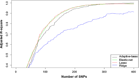
Figures 2–4 show the results of KARE data analysis. Figure 2 shows the adjusted R-square with the number of SNPs when SNPs are filtered by P-values. There is a tendency for the adjusted R-square to increase as the number of SNPs increases. The increase rate of the ridge method is slower than that of the IAL, lasso, and elastic-net methods. The adjusted R-squares all converge to 0.75 except for the ridge method. The IAL method shows the fastest increase rate.

Figure 3 shows the adjusted R-square with the number of SNPs when the SNPs are filtered by the absolute values of coefficients. There is a tendency for the adjusted R-square to increase as the number of SNPs increases. The increase rate of the ridge method is slower than that of other penalized regression methods. The adjusted R-squares all converge to 0.71 except for the ridge method. The IAL, lasso, and elastic-net methods show very similar increase rates.

Figure 4

Comparison of adjusted R-squares when SNPs are filtered out by P-value in KARE data analysis. The SNPs are ranked by effect size for each method.

Figure 5

Comparison of adjusted R-squares when the SNPs are filtered out by P-values in AREDS data analysis. The X-axis represents the number of SNPs and the Y-axis the adjusted R-squares. The SNPs are ranked by effect size for each method.

Figures 2 and 3 show the consistent results that (1) the P-value criterion tends to select better SNPs to predict the traits than the absolute values of coefficients criterion and (2) the ridge method performs worse in variable selection than other penalized regression methods.

Note that Figures 2 and 3 compare four penalized regression methods for a given pre-screening criterion. Among the IAL, lasso, and elastic-net methods, only the IAL method ranks SNPs by effect size. We wonder whether this difference among these three methods may be because of a different ordering of SNPs. Thus, instead of using BSS for the lasso and elastic-net methods, we use the same ordering of SNPs by effect size. Figure 4 shows the adjusted R-square with the number of SNPs when SNPs are filtered by the absolute values of the coefficients and ordered by effect size. Interestingly, the elastic-net, lasso, and IAL methods produce almost identical results. Thus, Figure 4 suggests that effect size is a better SNP ordering measure than BSS.

Areds Data

Figures 5 and 6 show the results of AREDS data analysis. These figures show very consistent results with those of KARE. Figure 5 shows the adjusted R-square with the number of SNPs when SNPs are filtered by P-values and ordered by effect sizes. There is a tendency for the adjusted R-square to increase as the number of SNPs increases. The increase rate of the ridge method is slower than that of the IAL, lasso, and elastic-net methods. The IAL, lasso, and elastic-net methods show very similar increase rates. Figure 6 shows the adjusted R-square with the number of SNPs when the SNPs are filtered by the absolute values of coefficients ordered by effect sizes. There is a tendency for the adjusted R-square to increase as the number of SNPs increases. The increase rate of the ridge method is slower than that of other penalized regression methods.

Figure 6

Comparison of adjusted R-squares when SNPs are filtered out by effect size in AREDS data analysis. The X-axis represents the number of SNPs and the Y-axis the adjusted R-squares. The SNPs are ranked by effect size for each method.

Conclusion

Recently many high-dimensional datasets have been generated in biomedical science, such as microarrays and SNP databases. Multistep strategies have been introduced to analyze these data. The first stage is pre-screening, in which the marginally associated response variables are identified, using various criteria. The second stage is variable selection. Various penalization methods have been proposed to analyze high-dimensional data. These include the ridge, bridge, least absolute shrinkage and selection operator (lasso), adaptive lasso, SCAD, and elastic-net methods. However, we do not know which method performs best for quantitative traits. Using an adjusted R-square as a measure of comparison, our study shows that for quantitative traits, the P-value criterion selects better variables to predict the trait than the absolute values of coefficients criterion. We conclude that the elastic-net, lasso, and IAL methods have almost the same performance, while the ridge method performs worst in variable selection.

In this study, we use only quantitative traits. However, a similar study could be easily conducted using binary traits such as diabetes and high blood pressure.

Because of gaps in the data, we unavoidably eliminate SNPs and individuals who have at least one missing value. This loss of information may reduce the accuracy of the study. We need to improve this accuracy by trialing appropriate imputation methods using simulated datasets.

Author Contributions

Conceived and designed the experiments: TP, SH. Analyzed the data: SH, YK. Wrote the first draft of the manuscript: TP, SH. Contributed to the writing of the manuscript: TP, SH, YK. Agree with manuscript results and conclusions: TP, SH, YK. All authors reviewed and approved of the final manuscript.

Footnotes

Acknowledgement

The AREDS data used for the analyses described in this manuscript were obtained from the AREDS database, controlled through the database of Genotypes and Phenotypes (dbGaP) accession number phs000001.v2.pl.

References

Cho

, Kim

Y.J.

. Joint identification of multiple genetic variants via elastic-net variable selection in a genome-wide association analysis. Ann of Hum Genet. 2010; 74: 416–28.

T.T.

, Chen

Y.F.

, Hastie

, Sobel

, Lange

Genome-wide association analysis by lasso penalized logistic regression. Bioinformatics. 2009; 25: 714–21.

Fan

, Lv

J.C.

Sure independence screening for ultrahigh dimensional feature space. J Roy Stat Soc B. 2008; 70: 849–911.

Fan

, Song

Sure independence screening in generalized linear models with NP-dimensionality. Ann Stat. 2010; 38: 3567–604.

Tibshirani

Regression shrinkage and selection via the lasso. J Roy Stat Soc B Met. 1996; 58: 267–88.

Zou

, Hastie

Regularization and variable selection via the elastic net. J Roy Stat Soc B Met. 2005; 67: 301–20.

Fan

, Li

Variable selection via nonconcave penalized likelihood and its oracle properties. J Am Stat Assoc. 2001; 96: 1348–60.

Le Cessi

, Van Houwelingen

J.C.

Ridge estimators in logistic regression. Ann Appl Stat. 1992; 41: 191–201.

Zou

The adaptive lasso and its oracle properties. J Am Stat Assoc. 2006; 101: 1418–29.

10.

Wei

, Joseph

G.I.

, Zou

Genomewide multiple-loci mapping in experimental crosses by iterative adaptive penalized regression. Genetics. 2010; 185(1): 349–59.

11.

Cho

, Go

, Kim

. A large-scale genome-wide association study of Asian populations uncovers genetic factors influencing eight quantitative traits. Nat Genet. 2009; 41: 527–34.

12.

The Age-Related Eye Disease Study Research Group. The age-related eye disease study (AREDS): design implications AREDS report no. 1. Control Clin Trials. 1999; 20(6): 573–600.

13.

Berndt

S.I.

, Gustafsson

, Mägi

. Genome-wide meta-analysis identifies 11 new loci for anthropometric traits and provides insights into genetic architecture. Nat Genet. 2013; 45(5): 501–12.

14.

Gudbjartsson

D.F.

, Walters

G.B.

, Thorleifsson

. Many sequence variants affecting diversity of adult human height. Nat Gent. 2008; 40(5): 609–15.

Practical Issues in Screening and Variable Selection in Genome-Wide Association Analysis

Abstract

Keywords

Introduction

Materials and Methods

Materials

KARE Data

Areds Data

Methods

Method 1

Method 2. IAL

Results

Pre-screening

KARE Data

Areds Data

Variable Selection

KARE Data

AREDS data.

Comparative Study

KARE Data

Areds Data

Conclusion

Author Contributions

Footnotes

Acknowledgement

References