Sage Journals: Discover world-class research

Abstract

The pathological description of the stage of a tumor is an important clinical designation and is considered, like many other forms of biomedical data, an ordinal outcome. Currently, statistical methods for predicting an ordinal outcome using clinical, demographic, and high-dimensional correlated features are lacking. In this paper, we propose a method that fits an ordinal response model to predict an ordinal outcome for high-dimensional covariate spaces. Our method penalizes some covariates (high-throughput genomic features) without penalizing others (such as demographic and/or clinical covariates). We demonstrate the application of our method to predict the stage of breast cancer. In our model, breast cancer subtype is a nonpenalized predictor, and CpG site methylation values from the Illumina Human Methylation 450K assay are penalized predictors. The method has been made available in the ordinalgmifs package in the R programming environment.

Keywords

methylation cancer ordinal response penalized regression

Introduction

Ordinal outcomes, or any outcome with inherent ordering, occur frequently in biomedical data. Examples of these types of ordered responses include severity of depression, grading of adverse events, the Knodell score for liver biopsies,¹ or stage of cancer. Stage of cancer is a pathological description of a tumor, and for breast cancer it considers the following: size of the tumor, number of cells in the tumor, location of tumor with respect to the chest wall and skin, the amount of cancer in mammary, axillary, and sentinal lymph nodes, the number of lymph nodes involved, and the spread of cancer to other organs.² Stage of cancer typically determines the course of therapy and is most often ascertained through a biopsy of the cancerous tissue. When modeling stage of cancer, it maybe of interest to predict which response level a patient may exhibit, given some set of explanatory variables. Ordinal regression may be used to model the probability of exhibiting a specific ordinal response, given some set of relevant covariates. However, ordinal regression methods require either that the sample size exceeds the number of features or that all covariate parameters be penalized. It is of interest here to develop a method that allows the model to penalize some covariates without penalizing others (such as demographic covariates).

In our research, we are interested in using high-dimensional methylation data from the Illumina Human Methylation 450K technology, in conjunction with other factors, to predict stage of cancer in a sample of women with breast cancer. Methylation is an epigenetic event that alters gene expression without altering the DNA sequence itself. It is the process by which a cytosine molecule on the DNA strand becomes a 5-methylcytosine through the addition of a methyl group, or a 5-hydroxymethylcytosine through the addition of a methyl group followed by a hydroxy group. Profound methylation changes are known to occur in the context of cancer; well-documented changes include the hypermethylation of tumor-suppressor genes³ and the hypomethylation of protooncogenes.⁴ Specific patterns of methylation exhibited in tumors are thought to not only detect cancer⁵ but also predict tumor behavior⁶ and illuminate differences and similarities across and within tumor types.³ Jones and Laird stated that perhaps methylation patterns in cells could serve as “a rough blueprint for the expression profile of that cell” and envisioned that future development of science and technology might produce a useful methylation analysis to generate a “DNA methylation fingerprint for a tumor biopsy.”⁷ Studies of methylation patterns in peripheral blood specimens from people diagnosed with cancer have also shown alterations. Of particular relevance, DNA methylation analysis from peripheral blood samples recently identified an association between methylation of the HYAL2 gene and breast cancer,⁸ suggesting that methylation patterns in blood might be useful as a screening tool for evaluating tumors in other tissues. Because epigenetic changes, such as methylation, are reversible, identification of specific methylation changes occurring in specific cancers may lead to targeted therapies to return normal function to the cells.⁷ Given this evidence, we hypothesized that differential methylation maybe predictive of stage of cancer in women with breast cancer.

Methods

Data

In this paper, we worked with one dataset from a breast cancer study conducted at Virginia Commonwealth University. This research was approved by the Institutional Review Board at Virginia Commonwealth University (VCU IRB #HM 13194) and complied with the principles of the Declaration of Helsinki. Our dataset included 73 women with breast cancer and included baseline clinical and demographic covariates such as estrogen receptor (ER), progesterone receptor (PR), and human epidermal growth factor receptor 2 (HER2) status, age, race (white or African-American), prior breast cancer surgery (lumpectomy, segmental, or simple surgery prior to study enrollment), and smoking status (currently smoking, yes or no). ER, PR, and HER2 status were collapsed into a single, categorical measure of breast cancer subtype,⁹ defined in Table 1.

Table 1.

Criteria for breast cancer subtype classification.

SUBTYPE	DEFINITION
Luminal A	ER+ and/or PR+, HER2−
Luminal B	ER+ and/or PR+, HER2+
Triple negative	ER−, PR−, HER2−
HER2 Type	ER−, PR−, HER2+

Notes: Breast cancer subtype classification typically considers proportion of tumor cells positive for the Ki67 protein. This measurement was not collected in our study and therefore could not be used for classification.

Peripheral blood samples were collected at study entry, and DNA was subsequently extracted from these samples using standard methods, bisulphite converted (Zymo Research EZ Methylation Kit), and hybridized to Illumina's Human Methylation 450K array according to the manufacturer's protocol. To assess assay reliability, some samples were hybridized multiple times, resulting in a total of 82 methylation profiles.

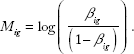
The scanned arrays were processed using the minfi¹⁰ Bioconductor package in the R programming environment to obtain the β-values for each probe, where β _ig represents the proportion methylated for the ith sample and the gth. CpG site, defined here as

β = \frac{M}{M + U + offset}

where M is the methylated signal for a given CpG site, U is the unmethylated signal for a given CpG site, and offset is 100, to avoid division by small numbers.¹¹

Some preprocessing of the methylation data was necessary prior to statistical analysis. Our first preprocessing step was to look at the distribution of β-values by the GC content. This is important because previous research has established that methylation may not be accurately measured in regions of high GC content.¹² Illumina's design for the 450K array includes two separate assays, Type I and Type II, for estimating methylation at a given locus. GC content was calculated as the proportion of the probe sequence comprised of C's and G's and reported separately for Type I and Type II design types. We then examined the boxplots of average β-values (across all samples) by the GC content for each of the assay types separately (Figs. 1 and 2). The resulting boxplots were used to determine a GC proportion cutoff value beyond which methylation seems to no longer be reliably measured. The choice of such a cutoff is clearly subjective, but it is important to remove the CpG sites beyond the cutoff because inclusion of unreliable probes may distort the analysis. We also removed CpG sites within which there were known single nucleotide polymorphisms (SNPs) according to the Illumina-provided annotation files.¹¹

Figure 1.

Boxplot of mean β-values by percent GC content across all samples, for type I probes.

Figure 2.

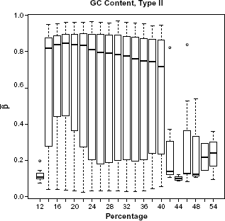
Boxplot of mean β-values by percent GC content across all samples, for type II probes.

The Type I design includes two bead types for each CpG site: one that detects methylated CpG sites, and the other that detects unmethylated CpG sites. The Type II design includes a single bead with a two-color readout; a different color is used to indicate whether the CpG site is methylated or unmethylated. In 2011, Dedeurwaerder et al examined the distribution of β-values produced by Type I and Type II bead types used in the 450K technology.¹³ They noted that the distribution of β-values from both bead types, across the whole array, exhibited two distinct peaks, one close to 0 for the unmethylated CpGs and one close to 1 for the methylated CpGs. These peaks, however, when modeled separately by bead type, did not align exactly; the peaks for the β-values from the Type II beads were shifted inwards when compared to the Type I beads. This shift is attributed to the difference in chemistry between the beads and is acknowledged by Illumina in a Technical Note for the 450K technology on their Web site.¹⁴ To correct this issue, we implemented the peak correction method by Dedeurwaurder et al on our β-values as a preprocessing step. This method adjusts the Type II peaks so that they align to the locations of the Type I peaks. The peak correction method uses the M-values and the logit of the β-values

M_{i g} = \log (\frac{β_{i g}}{(1 - β_{i g})}) .

Prior to the logit transformation and peak correction, we modified the β-values slightly by adding or subtracting 0.001 to any β-value exactly equal to 0 or 1, respectively, in order to prevent errors during the logit transformation.

Finally, there were five patients having n₁ = 4, n₂ = 4, n₃ = 2, n₄ = 2, and n₅ = 2 hybridized samples each. For each of these patients, we averaged the final peak-corrected M-values across the replicate samples and used this single, mean signal for each of these five patients in our analysis. All data analyses were conducted in R (version 3.1.0) utilizing the minfi¹⁰ (version 1.10.2), limma¹⁵ (version 3.16.8), VGAM (version 0.9–4),¹⁶ and ordinalgmifs¹⁷ (version 1.0.2) packages. In our analysis, we used the 450K annotation file version 1.2.¹⁸

Analysis

In genomic research, traditional modeling methods are often inappropriate. Traditional ordinal regression methods, for example, require that the number of predictors (p) be smaller than the sample size (n) and that the predictors be independent. After filtering, our breast cancer study included 353,331 CpG sites and only 73 patients; such a situation, where p >> n, is typical when analyzing high-throughput genomic data. Furthermore, we know that methylation levels of CpG sites in close proximity to one another are highly correlated. To handle these challenges, we implemented penalized regression methods. Penalized regression introduces bias into the model in exchange for reducing variability.¹⁹ The resulting model is sparse, which is an attractive feature when dealing with an overly large predictor space and we are interested in producing a parsimonious model.

There are a variety of algorithms available for finding a penalized solution. One such algorithm is the Incremental Forward Stagewise (IFS) method, which provides the monotone Least Absolute Shrinkage and Selection Operator (LASSO) solution in a linear regression setting.²⁰ Hastie et al modified and extended the IFS procedure, creating the generalized monotone incremental forward stagewise (GMIFS) method, which provides a penalized solution in a logistic regression setting.²⁰ Archer et al further extended the GMIFS method to provide the penalized solution in an ordinal regression setting.²¹ In our work, we extended the GMIFS algorithm to allow a subset of covariates to be included in the model without penalization.

This so-called no-penalty subset, the subset of demographic variables not penalized, is included in the final model, and the fitting algorithm is not allowed to shrink any of these coefficients to 0. This no-penalty subset option is important in many scientific investigations where some biologically relevant demographic information should be retained in the model, regardless of statistical significance ascribed to the given covariates. For our breast cancer dataset, we fit univariate ordinal response models predicting stage for each of the following: age, race, body mass index (BMI), smoking status, prior surgery related to the management of breast cancer, and subtype, to see which of these will be important for inclusion in the full ordinal model. We conducted a likelihood ratio test (LRT) to obtain the P-values for each of these univariate models. We used a P-value cutoff of 0.05 to determine which demographic covariates were important for inclusion in the no-penalty subset.

Given the large number of CpG sites in the 450K array, we first filtered the M-values by significance in order to reduce the number of penalized coefficients considered by the model. We fit a model with only the demographic covariates found to be important from the previous LRTs and each of the CpG sites individually. We then conducted a series of LRTs between the demographic-only model and each of the CpG site models. Using a liberal P-value threshold of 0.25, we included in the penalized model only those CpG sites with a P-value <0.25. Additionally, we removed CpG sites that were universally unmethylated (β < 0.1) across all samples and those that were universally methylated (β > 0.9) in all samples. Removing these CpG sites constituted no loss of information since all the samples were either fully unmethylated or fully methylated.

The primary outcome measure of interest, as mentioned, was stage of cancer. Stage of cancer is measured as 0—IV and may be further subdivided into 0, IA-B; IIA-B; IIIA-C; and IV The patients in our study, which focused on ascertaining participants with early stage breast cancer, were classified as stage I (n = 21), IIA (n = 29), IIB (n = 15), or IIIA (n = 8). We constructed a response matrix 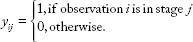y which was an n × k matrix representing class membership. For i = 1,…, n, subjects may take one of h = 1,…, k stages (ordinal levels), and the elements of the matrix are

y_{i j} = {\begin{cases} 1, if observation i is in stage j \\ 0, otherwise . \end{cases}

We also constructed a matrix of nonpenalized predictors 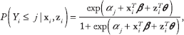z and a matrix of penalized predictors x. Using a cumulative logit model to model the k − 1 logits of ordinal categories at or below a given level, the probability of interest may be expressed as follows:

P (Y_{i} \leq j | x_{i}, z_{i}) = \frac{\exp (α_{j} + x_{i}^{T} β + z_{i}^{T} θ)}{1 + \exp (α_{j} + x_{i}^{T} β + z_{i}^{T} θ)},

where α _j 's represent the intercepts and β, and θ represent the coefficients for the penalized and nonpenalized predictors, respectively. In this way, we modeled the conditional probability that, given values of the demographic and methylation covariates, the cancer classification for a patient would fall at or below a certain stage. The conditional probability that the cancer classification would fall exactly at a certain stage may be written as

\begin{matrix} π_{j} (x_{i}, z_{i}) = P (Y_{i} = j | x_{i}, z_{i}) \\ = \frac{\exp (α_{j} + x_{i}^{T} β + z_{i}^{T} θ)}{1 + \exp (α_{j} + x_{i}^{T} β + z_{i}^{T} θ)} - \frac{\exp (α_{j - 1} + x_{i}^{T} β + z_{i}^{T} θ)}{1 + \exp (α_{j - 1} + x_{i}^{T} β + z_{i}^{T} θ)} \end{matrix}

Therefore, the likelihood is given by

L = \prod_{i = 1}^{n} \prod_{j = 1}^{J} π_{j} {(x_{i}, z_{i})}^{y_{i j}}

and the log-likelihood is given by

\log (L) = \sum_{i = 1}^{n} \sum_{j = 1}^{J} y_{i j} \log (π_{j} (x_{i}, z_{i}))

which can be more formally expressed as

\begin{array}{l} \log (L) = \sum_{i}^{n} \sum_{j}^{J} y_{i j} \log \\ (\frac{\exp (α_{j} + x_{i}^{T} β + z_{i}^{T} θ)}{1 + \exp (α_{j} + x_{i}^{T} β + z_{i}^{T} θ)} - \frac{\exp (α_{j - 1} + x_{i}^{T} β + z_{i}^{T} θ)}{1 + \exp (α_{j - 1} + x_{i}^{T} β + z_{i}^{T} θ)}) \end{array}

The specific steps of the modified GMIFS algorithm to obtain this solution are implemented in the ordinalgmifs package in R.¹⁷ We outline the steps for the cumulative logit form of the model here.

Beginning at step s = 0,

Augment the x covariate space by appending the negative of the covariate space so that x becomes [x: −x].^*

We augment the covariate space in this way so that we may avoid calculation of the second derivative to determine the direction of the update.²⁰

Set all of the β terms to 0 so that ${\hat{β}}^{(s)} = 0$ . (The β vector is of length 2p)

Initialize the α terms as $α_{j} = \log i t (\sum_{i = 1}^{n} \sum_{k = 1}^{j} \frac{y_{i j}}{n})$ .

Holding the β terms fixed, update α and θ by maximum likelihood.

Holding α and θ fixed, find $m = \underset{p}{\arg \min} - \frac{δ}{δ β_{p}} (\log L)$ .

Update ${\hat{β}}_{m}^{s + 1}$ to be ${\hat{β}}_{m}^{s + 1} + ε$ , where ∊ is some small value. We used ∊ = 0.01.

Repeat steps 4–6 until log L^(s+1) − log L^(s) < τ, where τ is some small value. We used τ = 0.00001.

Once the algorithm converges, the parameter estimates achieved constitute the “converged model.” For each step of the algorithm, we calculated the log likelihood, Akaike Information Criterion (AIC), and the Bayesian Information Criterion (BIC) for the model at that iteration of the algorithm. AIC and BIC are measures of the relative quality of a statistical model. We then extracted the parameter estimates at the step that minimized the AIC.

The penalized covariates are given by x, with β denoting the corresponding parameter estimates. As indicated in step 2 of the algorithm, at the first step all the β's are set to zero. For each consecutive step of the algorithm, only one β is updated by a very small incremental amount. As indicated in steps 5 and 6 of the algorithm, the β that is updated is that which corresponds to the predictor having the largest negative derivative of the log likelihood. After a β has been updated, the thresholds and unpenalized predictors are estimated by maximum likelihood keeping the β fixed (see step 4 of the algorithm). For this reason, some predictors are penalized (x) while others are not penalized (z). The penalized β estimates are found when the log likelihood is minimized with respect to the following constraints:

β_{g}^{+}, β_{g}^{-} \geq 0 and \sum_{g = 1}^{G} (β_{g}^{+} + β_{g}^{-}) \leq s

The value of s is not specified by the user. Rather, each of the s values corresponds to a specific solution²⁰ so that both the AIC-selected and the converged model will have an associated s value. Note that this method is an incremental forward stagewise method, which differs from preselecting a tuning parameter, or set of tuning parameters, against which the model is fit, then subsequently selecting the best fitting model by some model-fitting criterion.

For our selected model, we were interested in how the blood methylation values predicted the stage of the actual tumor. For the nonzero coefficient estimates, we investigated whether any of the differentially methylated loci had been previously associated with breast cancer or other types of cancer.

Simulation Study

We also conducted a simulation study to further test the performance of the method. Currently, there exists no comparative method that fits a penalized cumulative logit model, so we have no method against which to test the GMIFS cumulative logit model performance. For our simulation study, we used a sample size of 80 subjects, where 100 predictor variables were generated from a uniform distribution on the [−1, 1] interval. Thereafter, the latent response, 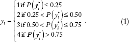$y_{i}^{*}$ for i = 1,…, 80, was generated by using the first four predictors (X₁,…, X₄) as covariates truly associated with the response where the coefficients were (0.5, −0.5, 0.5, −0.5) and adding a Gaussian error term with mean 0 and standard deviation of 0.15. The observed response was generated by referencing the probabilities of the generated latent response using a standard normal distribution, where the observed class was taken to be

y_{i} = {\begin{cases} 1 if P (y_{i}^{*}) \leq 0.25 \\ 2 if 0.25 < P (y_{i}^{*}) \leq 0.50 \\ 3 if 0.50 < P (y_{i}^{*}) \leq 0.75 \\ 4 if P (y_{i}^{*}) > 0.75 \end{cases} .

(1)

Thereafter, a cumulative logit GMIFS model was fit using X₁ as an unpenalized predictor and X₂, X₃ X₄ as penalized predictors and the AIC selected model was examined. This entire process was repeated 50 times. Characteristics of the fitted models examined included the number of times the coefficients for X₂, X₃, and X₄ were nonzero (true positive rate); the number of times the coefficients for X₅,…, X₁₀₀ were nonzero (false positive rate); and the misclassification rate.

Our simulation study indicated that the method performed well. The true positive rate was 100%, as all models returned nonzero coefficient estimates for X², X₃ and X₄. The median false positive rate was 5.2% (range 0–33%). The median misclassification rate was 13.75% (range 1.25–30.00%).

Results

Table 2 provides an overview of the distribution of the continuous and binary demographic covariates by stage of cancer. Table 3 provides the distribution of the multi-level categorical covariate.

Table 2.

Demographic characteristics by stage of cancer. The medians are reported for continuous variables (age and BMI) and the frequencies are reported for categorical variables (race, smoking status, and prior surgery).

STAGE	I n = 21	IIA n = 29	IIB n = 15	IIIA n = 8	TOTAL n = 73
Age (median)	55	48	56	49	53
BMI (median)	29.58	25.79	31.01	29.25	28.34
Race (Black)	5/21	10/29	6/15	0/8	21/73
Currently smoking (Y)	3/21	5/29	6/15	1/8	15/73
Prior surgery (Y)	21/21	26/29	12/15	7/8	66/73

Table 3.

Frequencies of breast cancer subtype by stage of cancer.

STAGE	I n = 21	IIA n = 29	IIB n = 15	IIIA n = 8	TOTAL n = 73
Luminal A	7	16	7	7	37
Luminal B	2	3	3	0	8
Triple negative	11	7	2	1	21
HER2 type	1	3	3	0	7

The original, unfiltered data had 485,512 CpG sites. The boxplots of GC content by CpG site (Figs. 1 and 2) indicate that methylation may not be accurately measured beyond 42% for Type I probes or beyond 40% for Type II probes. After examining these boxplots, we chose the more conservative of the two values and excluded CpG sites with greater than 40% GC content from further analysis. This GC content filtering criteria removed 52,077 CpG sites, leaving 433,435 CpG sites. Next we removed the 80,104 CpG sites that included SNPs, leaving 353,331 CpG sites. There were 1,742 β-values exactly equal to 0, while none were exactly equal to 1. We imputed those equal to 0 to be 0.001 before applying the logit transform. After this, we applied the peak correction method to align the Type II peaks to the locations of the Type I peaks. An LRT was conducted for each of the demographic covariates comparing the intercepts-only model to each of the univariate models when fitting cumulative logit models to predict stage of cancer. The results of these tests are given in Table 4.

Table 4.

LRT and resulting P-values from univariate cumulative logit models predicting stage of cancer.

	INTERCEPTS ONLY	AGE	BMI	RACE	CURRENTLY SMOKING	PRIOR SURGERY	SUBTYPE
Deviance $χ_{1}^{2}$ statistic	188.72	187.57 1.15	188.70 0.02	188.69 0.03	187.56 1.16	185.70 3.02	179.91 8.81^*
P-Value		0.2834	0.8787	0.8611	0.2821	0.0824	0.0319

INTERCEPTS ONLY

AGE

BMI

RACE

CURRENTLY SMOKING

PRIOR SURGERY

SUBTYPE

Deviance

χ_{1}^{2}

statistic

188.72

187.57

1.15

188.70

0.02

188.69

0.03

187.56

1.16

185.70

3.02

179.91

8.81^*

P-Value

0.2834

0.8787

0.8611

0.2821

0.0824

0.0319

Note: *

$χ_{3}^{2}$ statistic.

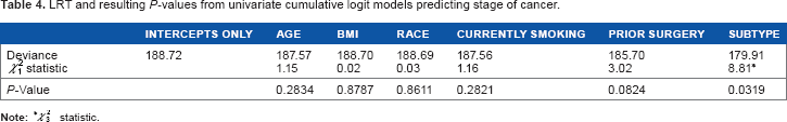
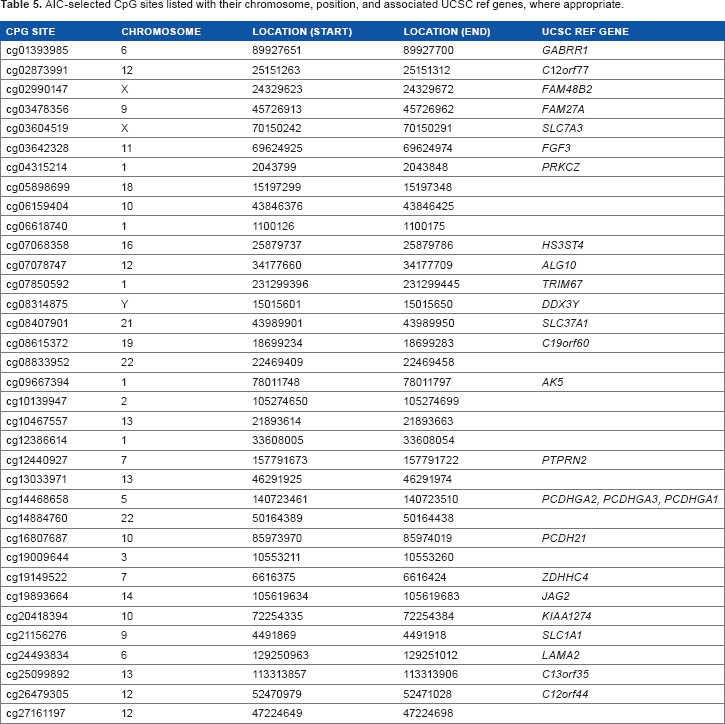
In the interest of developing a parsimonious model, we used a P-value cutoff of 0.05. At this significance level, it was clear that only subtype (eg, Luminal A; Luminal B; HER2+; triple negative) was significantly related to stage of breast cancer in this univariate sense. A similar LRT was conducted for each of the 353,331 CpG sites using the filtered, peak-corrected β-values. The model for the LRTs included only the demographic variable for cancer subtype. After excluding CpG sites with P-values greater than 0.25, 103,001 CpG sites remained. Finally, after excluding CpG sites for which the β-value was <0.1 or >0.9 in all samples, 27,110 CpG sites remained. The ordinal cumulative logit GMIFS model was fit to the subtype covariate as a nonpenalized predictor and to the M-values for the 27,110 CpG sites as penalized predictors. The model attaining minimum AIC included 35 nonzero CpG sites (Table 5), while the fully converged model estimated 107 nonzero CpG sites. Subsequently, we ran the model again, this time filtering to exclude CpG sites with P-values greater than 0.05. Fitting the same GMIFS model to this smaller set of CpG sites resulted in exactly the same parameter estimates and class predictions as the previous model, which used a P-value cutoff of 0.25.

Table 5.

AIC-selected CpG sites listed with their chromosome, position, and associated UCSC ref genes, where appropriate.

CPG SITE	CHROMOSOME	LOCATION (START)	LOCATION (END)	UCSC REF GENE
cg01393985	6	89927651	89927700	GABRR1
cg02873991	12	25151263	25151312	C12orf77
cg02990147	X	24329623	24329672	FAM48B2
cg03478356	9	45726913	45726962	FAM27A
cg03604519	X	70150242	70150291	SLC7A3
cg03642328	11	69624925	69624974	FGF3
cg04315214	1	2043799	2043848	PRKCZ
cg05898699	18	15197299	15197348
cg06159404	10	43846376	43846425
cg06618740	1	1100126	1100175
cg07068358	16	25879737	25879786	HS3ST4
cg07078747	12	34177660	34177709	ALG10
cg07850592	1	231299396	231299445	TRIM67
cg08314875	Y	15015601	15015650	DDX3Y
cg08407901	21	43989901	43989950	SLC37A1
cg08615372	19	18699234	18699283	C19orf60
cg08833952	22	22469409	22469458
cg09667394	1	78011748	78011797	AK5
cg10139947	2	105274650	105274699
cg10467557	13	21893614	21893663
cg12386614	1	33608005	33608054
cg12440927	7	157791673	157791722	PTPRN2
cg13033971	13	46291925	46291974
cg14468658	5	140723461	140723510	PCDHGA2, PCDHGA3, PCDHGA1
cg14884760	22	50164389	50164438
cg16807687	10	85973970	85974019	PCDH21
cg19009644	3	10553211	10553260
cg19149522	7	6616375	6616424	ZDHHC4
cg19893664	14	105619634	105619683	JAG2
cg20418394	10	72254335	72254384	KIAA1274
cg21156276	9	4491869	4491918	SLC1A1
cg24493834	6	129250963	129251012	LAMA2
cg25099892	13	113313857	113313906	C13orf35
cg26479305	12	52470979	52471028	C12orf44
cg27161197	12	47224649	47224698

Boxplots (Figs. 3 and 4) are shown for the two CpG sites from Table 5 with the largest absolute coefficient. The plots display the distribution of β-values for all subjects according to stage of cancer. The β-values for cg19149522 (ZDHHC4) seem to be monotonically decreasing, while the β-values for cg16807687 (PCDH21) seem to be monotonically increasing.

Figure 3.

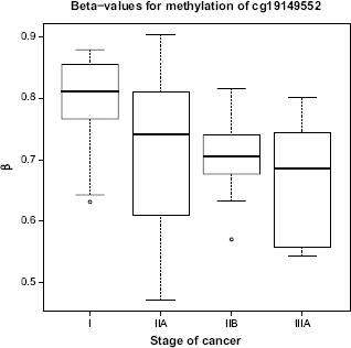
Boxplot of β-values for CpG site cg19149522 (ZDHHC4), for ail subjects, by stage of cancer.

Figure 4.

Boxplot of β-values for CpG site cg16807687 (PCDH21), for all subjects, by stage of cancer.

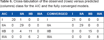
The fully converged model predicted the stage without error, while the minimum AIC model had an error rate of 15.1%. Table 6 shows the cross-tabulation of observed versus predicted class. The fully converged model was without error; however, it included 107 nonzero parameter estimates indicating that it is likely overfit. The AIC model was less accurate for prediction, particularly for patients with stage IIIA cancer. This is likely due to the fact that our patient sample is unbalanced across the stages and is biased toward stages I–IIB.

Table 6.

Cross-tabulation of the observed (rows) versus predicted (columns) class for the AIC and the fully converged models.

AIC	I	IIA	IIB	IIIA	CONVERGED	I	IIA	IIB	IIIA
I	220	1	0	0	I	21	0	0	0
IIA	0	29	0	0	IIA	0	29	0	0
IIB	0	4	11	0	IIB	0	0	15	0
IIA	0	0	6	2	IIIA	0	0	0	8

Discussion

In this paper, we presented an ordinal response model for high-dimensional covariate spaces that allows the inclusion of nonpenalized covariates, penalized covariates, or both. This method can be applied to any cumulative link, forward continuation ratio, backward continuation ratio, adjacent category, or stereotype logit model using the ordinalgmifs R package.¹⁷ While the fully converged model had 100% accuracy in predicting stage of cancer, there were several misclassifications for the AIC-selected model. This may be partially attributed to the imbalance and small class size, particularly for stage IIIA. However, several of the CpG sites included in the models were located within genes that have previously been associated with breast cancer. AK5, PTPRN2, LAMA2, FGF3, SLC37A1, and SLC1A1 have all been previously associated with breast cancer.^22–28 SLC7A3, PRKCZ, JAG2, GABRR1, DDX3Y, and PCDHGA3 have been previously associated with other types of cancer.^29–34 Our results, which agree with previously published results, indicate that methylation patterns of the tumor itself may impact the methylation patterns present in peripheral blood. Development of a model that can accurately predict stage of cancer from DNA methylation or other genomic profiles from peripheral blood samples and demographic information may have important healthcare implications. We hope that our work here will help future development of less invasive, less expensive methods for determining the stage of cancer.

Author Contributions

Conceived of this study: KJA. Planned the data collection and subject recruitment: CKJC, DEL. Analyzed the data: AEG, KJA. Wrote the first draft of the manuscript: AEG. Contributed to the writing of the manuscript: CKJC, DEL, KJA. Agree with manuscript results and conclusions: AEG, CKJC, DEL, KJA. Jointly developed the structure and arguments for the paper: AEG, KJA. Made critical revisions and approved final version: CKJC, DEL, KJA. All authors reviewed and approved of the final manuscript.

Footnotes

Acknowledgments

Research reported in this publication was supported by the National Library of Medicine of the National Institutes of Health under Award Number R01LM011169. Data collection was supported by the National Institute of Nursing Research of the National Institutes of Health under Award Number R01NR012667. Support was also provided under award number R25DA026119 from National Institute on Drug Abuse. Services in support of the research project were generated by the VCU Massey Cancer Center Biostatistics Shared Resource, supported, in part, with funding from NIH-NCI Cancer Center Support Grant P30 CA016059. The content is solely the responsibility of the authors and does not necessarily represent the official views of the National Institutes of Health.

References

Knodell

R.G.

, Ishak

K.G.

, Black

W.C.

Formulation and application of a numerical scoring system for assessing histological activity in asymptotic chronic active hepatitis. Hepatology. 1981; 1: 431–5.

American Cancer Society. How is breast cancer staged? 2014. Available at: http://www.cancer.org/cancer/breastcancer/detailedguide/breast-cancer-staging. Accessed November 19, 2014.

Eng

, Herman

J.G.

, Baylin

S.B.

A bird's eye view of global methylation. Nat Genet. 2000; 24: 101–2.

Ehrlich

DNA methylation in cancer: too much, but also too little. Oncogene. 2002; 21: 5400–13.

Baylin

S.B.

, Belinsky

S.A.

, Herman

J.G.

Aberrant methylation of gene promoters in cancer – concepts, misconcepts, and promise. J Natl Cancer Inst. 2000; 92: 1460–1.

Baylin

S.B.

, Esteller

, Rountree

M.R.

, Bachman

K.E.

, Schuebel

, Herman

J.G.

Aberrant patterns of DNA methylation, chromatin formation and gene expression in cancer. Hum Mol Genet. 2001; 10: 687–92.

Jones

P.A.

, Laird

P.W.

Cancer epigenetics comes of age. Nat Genet. 1999; 21: 163–7.

Yang

, Pfütze

, Zucknick

DNA methylation array analyses identified breast cancer-associated HYAL2 methylation in peripheral blood. Int J Cancer. 2014; 136(8): 1845–55.

Susan

Komen. Breast cancer subtypes. 2014. Available at: http://ww5.komen.org/BreastCancer/SubtypesofBreastCancer.html. Accessed November 25, 2014.

10.

Aryee

M.J.

, Jaffe

A.E.

, Corrada-Bravo

Minfi: a flexible and comprehensive bioconductor package for the analysis of infinium DNA methylation microarrays. Bioinformatics. 2014; 30: 1363–9.

11.

Bibikova

, Barnes

, Tsan

High density DNA methylation array with single CPG site resolution. Genomics. 2011; 98: 288–95.

12.

Kuan

P.F.

, Wang

, Zhou

, Chu

A statistical framework for Illumina DNA methylation arrays. Bioinformatics. 2010; 26: 2849–55.

13.

Dedeurwaerder

, Defrance

, Calonne

, Denis

, Sotiriou

, Fuks

Evaluation of the infinium methylation 450k technology. Epigenomics. 2011; 3: 771–84.

14.

Infinium^®. HumanMethylation450 BeadChip Achhieves Breadth of Coverage Using Two Infinium^® Chemistries. San Diego, CA: Illumina, Inc.; 2012. http://res.illumina.com/documents/products/technotes/technote_hm450_data_analysis_optimization.pdf

15.

Smyth

G.K.

Limma: linear models for microarray data. In: Gentleman

, Carey

, Dudoit

, Irizarry

, Huber

eds. Bioinformatics and Computational Biology Solutions Using R and Bioconductor. New York: Springer; 2005: 397–420.

16.

Yee

T.W.

VGAM: Vector Generalized Linear and Additive. R Package Version 0.9-4. http://CRAN.R—project.org/package=VGAM. Published 2014.

17.

Archer

K.J.

ordinalgmifs: Ordinal Regression for High-Dimensional Data. R Package Version 1.0.2. http://CRAN.Rproject.org/package-ordinalgmifs. Published 2014.

18.

Illumina. Illumina Infinium Human Methylation 450k Manifest, Version 1.2; 2014. http://support.illumina.com/downloads/humanmethylation450_15017482_v1-2_product_files.html; 2014. Accessed July 22, 2014.

19.

Hastie

, Tobshirani

, Friedman

The Elements of Statistical Learning: Data Mining, Inference, and Prediction. 2nd ed. California: Springer; 2009. [ISBN 978-0-387-84857-0].

20.

Hastie

, Taylor

, Tibshirani

, Walther

Forward stagewise regression and the monotone lasso. Electron J Stat. 2007; 1: 1–29.

21.

Archer

K.J.

, Hou

, Zhou

, Ferber

, Layne

J.G.

, Gentry

A.E.

ordinalgmifs: ordinal regression for high-dimensional data. Cancer Inform. 2014; 13: 187–195.

22.

Miyamoto

, Fukutomi

, Askashi-Tanaka

Identification of 20 genes aberrantly methylated in human breast cancers. Int J Cancer. 2005; 116: 407–14.

23.

Nordgard

S.H.

, Johansen

F.E.

, Alnaes

G.I.

Genome-wide analysis identifies 16q deletion associated with survival, molecular subtypes, mRNA expression, and germline haplotype in breast cancer patients. Genes Chromosomes Cancer. 2008; 47: 680–96.

24.

Lee

, Oh

, Chung

Indentification of GABRA1 and LAMA2 as new DNA methylation markers in colorectal cancer. Int J Oncol. 2012; 40: 889–98.

25.

Mefford

, Mefford

Stromal genes add prognostic information to proliferation and histoclinical markers: a basis for the next generation of breast cancer gene signatures. PLoS One. 2012; 7: e37646.

26.

Roy

, Calaf

G.M.

Allelic loss at chromosome 11q13 alters FGF3 gene expression in a human breast cancer progression model. Oncol Rep. 2014; 32: 2445–52.

27.

Iacopetta

, Lappano

, Cappello

A.R.

SLC37A1 gene expression is up-regulated by epidermal growth factor in breast cancer cells. Breast Cancer Res Treat. 2010; 122: 755–64.

28.

Beaudin

S.G.

, Robilotto

, Welsh

Comparative regulation of gene expression by 1,25-dihydroxyvitamin D3 in cells derived from normal mammary tissue and breast cancer. J Steroid Biochem Mol Biol. 2015; 148: 96–102.

29.

Januchowski

, Zawierucha

, Andrzejewska

, Rucinski

, Zabel

Microarray-based detection and expression analysis of ABC and SLC transporters in drug-resistant ovarian cancer cell lines. Biomed Pharmacother 2013; 67: 240–5.

30.

Fransson

, Abel

, Kogner

, Martinsson

, Ejeskär

Stage dependent expression of pi3k/akt-pathway genes in neuroblastoma. Int J Oncol. 2013; 42: 609–16.

31.

Ory

, Tassi

, Cavalli

L.R.

The nuclear coactivator amplified in breast cancer 1 maintains tumor-initiating cells during development of ductal carcinoma in situ. Oncogene. 2014; 33: 3033–42.

32.

Oczko-Wojciechowska

, Wloch

, Wiench

Gene expression profile of medullary thyroid carcinoma – preliminary results. Endokrynol Pol. 2006; 57: 420–6.

33.

Karyagyna

A.S.

, Vassiliev

M.O.

, Ershova

A.S.

, Nurtdinov

R.N.

, Lossey

I.S.

Probe-level universal search (plus) algorithm for gender differentiation in affymetrix datasets. J Bioinform Comput Biol. 2010; 8: 553–77.

34.

Miller

, Rogers

H.A.

, Lyon

Genome-wide molecular characterization of central nervous system primitive neuroectodermal tumor and pineoblastoma. Neuro Oncol. 2011; 13: 866–79.

Penalized Ordinal Regression Methods for Predicting Stage of Cancer in High-Dimensional Covariate Spaces

Abstract

Keywords

Introduction

Methods

Data

Analysis

Simulation Study

Results

Discussion

Author Contributions

Footnotes

Acknowledgments

References