Sage Journals: Discover world-class research

Abstract

We have developed a general framework to construct an association network of single nucleotide polymorphisms (SNPs) (SNP association network, SAN) based on the functional interactions of genes located in the flanking regions of SNPs. SAN, which was constructed based on protein-protein interactions in the Human Protein Reference Database (HPRD), showed significantly enriched signals in both linkage disequilibrium (LD) and long-range chromatin interaction (Hi-C). We used this network to further develop two methods for predicting and prioritizing disease-associated genes from genome-wide association studies (GWASs). We found that random walk with restart (RWR) using SAN (RWR-SAN) can greatly improve the prediction of lung-cancer-associated genes by comparing RWR with the use of network in HPRD (AUC 0.81 vs 0.66). In a reanalysis of the GWAS dataset of age-related macular degeneration (AMD), SAN could identify more potential AMD-associated genes that were previously ranked lower in the GWAS study. The interactions in SAN could facilitate the study of complex diseases.

Keywords

genome-wide association study protein interaction network single nucleotide polymorphism random walk with restart

Introduction

In the last 10 years, genome-wide association studies (GWASs) have become an important approach for unbiased discovery of common genomic loci, represented by selected single-nucleotide polymorphisms (SNPs) that are associated with complex diseases or traits.^1,2 Associations between common SNPs and various diseases have been extensively studied,^3–6 but most of them either have small effects on disease risk or only explain a small fraction of the susceptible population.^7,8 In a typical GWAS analysis, a large number of SNPs are evaluated for their statistical associations with a certain phenotype.⁹ But, because of the need for multiple testing corrections, only very few SNPs can successfully surpass the significance threshold and be selected for the further investigation.^10,11 In such a context, one is very likely to miss some crucial information contained in the filtered-out SNP data. On the other side, since many complex diseases are the outcome of the joint action of multiple genes, many real biomarkers that have a significant risk effect in combination but not individually often fail to be detected by a typical GWAS.^12,13 Thus, there has been increasing demand in developing methods to reanalyze GWAS datasets and to study associations of high-order SNP combinations with complex phenotypes.^14,15

Recently, a gene-level knowledge-based strategy that utilizes prior biological knowledge at the gene level to facilitate GWAS dataset analysis has emerged as a potentially more powerful approach. One of the first attempts to utilize genetic information is gene-based GWAS analysis, in which all SNPs within a candidate gene are considered jointly.¹⁶ The pioneering method to combine SNPs in multiple genes is pathway-based GWAS analysis, in which SNPs located in diverse genes of the same pathway are examined jointly for their association with a disease or trait.¹⁷ In this method, genes in a specific pathway are treated as an exchangeable set. In a newly developed pathway-based method, a Markov random field model was proposed to incorporate the topological structure information of a pathway.¹⁸ Considering that current data sources of pathway cover only less than 20% of proteins and genes, network-based approaches on a larger scale have recently been developed to integrate network information to prioritize genes.^19,20

In this paper, we make an attempt in an alternative direction on how to reasonably utilize the genetic information to assist GWAS dataset analysis. Different from previous gene-based approaches that usually first map an SNP to a gene, we establish a general framework to map different sources of gene interaction information (such as protein-protein interaction, gene coexpression, or any types of functional associations) to SNP-tagged genomic loci, and sequentially construct a mutual SNP association network based on this information. Proven by large-scale experiment datasets (such as HapMap²¹ and HiC²²) and known disease-related SNP data,²³ this SNP association network (SAN) is able to reflect the real functional associations between genomic loci, which may facilitate the analysis of GWAS datasets. In order to test this, we developed a disease-related SNP prediction method by the use of a random walk with restart (RWR) strategy.²⁴ Compared with the prediction based on the Human Protein Reference Database (HPRD) network, the prediction based on SAN shows a significant improvement (AUC: 0.81 vs 0.66). We further test our SAN by reanalyzing the GWAS dataset of age-related macular degeneration (AMD).²⁵ By referring to Google's PageRank algorithm, we developed a new method that combined the AMD GWAS dataset with the SAN topological information to rerank the relevance between SNPs and AMD. According to our reranking result, we found new AMD-related SNP candidates, which is in agreement with reports in the literature.

Result

General Idea of SNP Association Network Construction

In GWASs, when an SNP is connected with a specific disease, it actually means that the chromosomal region around this SNP has one or more function elements, such as protein-coding genes, that are related to this disease.²⁶ Considering that those genes that are involved in the same disease tend to have closer functional interactions in the gene interaction network (GIN) than other genes,²⁷ we can exploit the gene interaction information to evaluate functional associations between genomic loci. Figure 1 shows a simple example of how SAN is constructed for three SNP-tagged genomic loci based on gene interactions. We can calculate the SNP association score (SAS, Formula 1 in the Method section) between each pair of SNPs and obtain a symmetric SAS matrix for all SNP pairs. SAS is calculated based on the connectivity between genes inside of the loci. The higher the score, the more the possibility that is there a functional association between these two loci. For this SAS matrix, we can further test the significance of each SAS by random permutation. After filtering out SNP pairs with nonsignificant SAS, we can finally construct the SAN.

Figure 1.

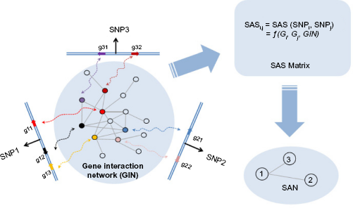
The general idea of SAN construction: an example network. G_i (or G_j) represents a gene set in the chromosomal region of SNP_i (or SNP_j). The computing method for SAS is as shown in Formula 1.

Parameter Setting for the SNP Association Network Construction

Several parameters need to be set in the construction of SAN in order to best utilize the information. The first parameter is the length of the genomic locus that each SNP represents. Based on the datasets of known disease-related genes and SNPs that are involved in coronary heart disease, prostate cancer, and schizophrenia, we tested variable lengths of genomic range (from 1 K to 1M). As shown in Figure 2A, when the length is increased, more disease-related genes can be embraced into the represented neighboring region of the known disease-associated SNPs; at the same time, the proportion of disease-related genes among total genes is decreased. We finally chose 100 kb (50 kb each from upstream and downstream of a SNP site) as the neighborhood of this SNP to balance both the coverage and specificity of disease-related genes in the SNP-represented regions. Furthermore, we clustered SNPs whose neighborhoods cover the same gene set into one SNP cluster, as they could not be distinguished in the calculation of functional association. Hence, in the SAN, an SNP cluster can be labeled as one node and represents one genomic locus.

Figure 2.

(A) Percentages (y-axis) of SNPs with disease-related genes located in varied flanking regions (x-axis) of either known disease-related SNPs (DS, pink) or randomly selected SNPs (DSR, red). It also shows the percentages of disease-related genes located in the varied length of flanking regions (x-axis) of either DS (DG, yellow) or DSR (DGR, blue). The disease-related genes and SNPs were collected from coronary heart disease. We found similar patterns in prostate cancer and schizophrenia also. (B) Cumulative distribution of negative log-transformed diffusion kernel scores between the disease-related genes (red) and genes from random background with the same degree in SAN (blue). (C) The impact of different SAS P-value thresholds on the size of SAN. (D) The degree distribution of the SAN. P(k) ~ k^−1.87; R² = 0.84. (E) The SAN in a circular layout. The four rings from outside to inside are ordered by (a) all human chromosomes, including 1–22 autosomes, X and Y chromosome, in units of 1M, (b) the density of SNPs, (c) the density of genes, and (d) the density of SAN edges. The inside lines represent SAN edges between chromosome loci in 1M unit; the increased linking numbers are represented by grey, red, orange, yellow, green, blue, and purple in order.

The second parameter is a control parameter in the diffusion kernel method.²⁸ In order to control the noise and to capture the long-range relationships between genes, we used the diffusion kernel method (Formula 2)²⁸ to transfer the HPRD network²⁹ into an inter-gene association matrix. In the diffusion kernel formula, the parameter β controls the extension of “diffusion”. To obtain an optimal value of β for multiple diseases, we tested different β values (from 0.01 to 2) using known disease-related genes from coronary heart disease, prostate cancer, and schizophrenia (Fig. 2B). Compared with random background, genes involved in a certain disease are likely to be connected closely, that is, larger scores in the diffusion kernel matrix. We chose 0.5 as the optimal β value because it gives the largest differences of cumulative distributions of diffusion kernel scores between disease-related genes from these three diseases and random background.

The third parameter is the P-value cutoff for selecting the statistically significant associations. Because different genomic loci contain different numbers of genes, which also have different degrees in the HPRD network, we cannot compare the SASs with each other directly. So for the SAS of each SNP cluster pair, we use permutation to generate a random background distribution and convert each SAS into an empirical P-value (Formula 3). The significant SASs can be determined based on a P-value cutoff. As shown in Figure 2C, we assessed the impact of different P-value thresholds on the size of the SAN and chose a P-value less than 1 × 10⁻⁴ as the threshold for further study.

In this way, we obtained a SAN with 13,217 nodes (genomic loci) and 153,235 interactions (significant associations). According to the distribution of degrees, the SAN is approximately a scale-free network,³⁰ which means there are hub nodes in the network (Fig. 2D). These hub nodes represent the hotspots on chromosomes, which tend to have more interactions with other genomic loci. In the circular layout³¹ of SAN (Fig. 2E), we can find that those hotpots are mainly located on chr1, chr11, chr12, chr17, and chr19. The density of interactions in the genome is positively correlated with the gene density (ρ = 0.53, P < 2.2 × 10⁻¹⁶, Spearman correlation test), but with no significant correlation to the density of SNP in the genome (ρ = −0.035, P = 0.092, Spearman correlation test).

Linkage Disequilibrium of SNP Cluster Nodes in the SNP Association Network

In population genetics, linkage disequilibrium (LD) is the nonrandom association of alleles at different loci on chromosomes.³² In the human genome, adjacent SNPs mostly have strong LD, forming the so-called LD block, whereas SNPs on different chromosomes or SNPs on the same chromosome but with long distance are not. In the SAN, about 92% of the interactions are inter-chromosomal while only 8% are intra-chromosomal. Interestingly, although most of the interacting nodes in the SAN are located on different chromosomes that do not exist in proximal LD blocks, they are likely to have a stronger LD compared with background distribution (Fig. 3A, P-value of Kolmogorov–Smirnov test (KS test) < 2.2 × 10⁻¹⁶, genotype data from HapMap). In the SAN, the median of LD between interacting nodes is 0.151, while the random background is 0.098 (P-value of Wilcox test < 2.2 × 10⁻¹⁶). The significantly stronger LD of interacting node pairs in the SAN raises the possibility that these node pairs are likely to have profound associations with similar functions or phenotypes.

Figure 3.

(A) Cumulative distribution of linkage disequilibrium score (R²) between randomly picked SNP cluster pairs (Background, green), SNP cluster pairs interacting in SAN (Network, red), and SNPs in one SNP cluster (Local, blue). For each SNP cluster pair, we calculated R² for all SNP pairs between the two SNP clusters in the pair, and used the maximum as R² for this SNP cluster pair. (B) LD blocks between SNP clusters SC13676 and SC5103. Pale red: r² > 0.1, deep red: r² > 0.2. Each row or column stands for an SNP.

Figure 3B shows a representative example of LD between two connected SNP cluster nodes SC13676 (on chromosome 7) and SC5103 (on chromosome 2). Both SC13676 and SC5103 have existing LD blocks in their own loci. Interestingly, the SNP pairs between these two loci, which are on different chromosomes, also display strong LD. There are two genes, TWIST1 and GLI2, on the corresponding genomic loci, respectively. TWIST1 and GLI2 do not interact directly in the HPRD network; they are coupled by the gene GLI3. Both GLI2 and GLI3 are members of GLI family of transcription factors and are crucial actors for normal development in the Sonic hedgehog–Patched–Gli (Shh-Ptch-Gli) pathway.^33,34 Dysregulation of the Shh-Ptch-Gli pathway leads to several human diseases, including birth defects and cancers.^35,36 Recent researches have shown that TWIST, a developmental regulatory gene and potential oncogene, does appear to be linked to Shh signal transduction.^37,38 Mouse Twist protein can activate transcription of human GLI1, another member of GLI family of transcription factors, by interacting with the E-boxes in GLI1's first intron.³⁹ More interestingly, nonsense, missense, deletion, and insertion mutations in several regions of the human TWIST gene have been shown to cause the Saethre–Chotzen syndrome, an autosomal dominant disease whose clinical phenotype partially overlaps with Shh-pathway-related human diseases.^40,41 All of these facts indicate that there is a strong functional association between these two genomic loci (represented by SC13676 and SC5103), which is well worth further joint analysis.

HiCinteraction between SNP Cluster Nodes in the SNP Association Network

The functional association of genomic loci with long distance in the genome may also connect with the direct long-range physical interaction of chromatins. The three-dimensional folding of chromosomes can bring distant functional elements such as a promoter and an enhancer into close spatial proximity. Such long-range interaction can be detected by the recently developed HiC technique in an unbiased and genome-wide manner.²² Here, we compared the genomic loci pairs that have direct interactions in the SAN with that in the human HiC data (Table 1). It was shown that, compared with randomly selected genomic loci pairs, the long-range chromatin interactions detected by HiC exhibit a clear dominance in genomic loci pairs that are directly interacting in the SAN (KS test P-value < 2.2 × 10⁻¹⁶). About 30% of the interacting SNP cluster pairs in the SAN can be found with HiC interactions. This frequency reduces to about 20% in the random background and increases to 40% for interacting SNP cluster pairs related to the same disease. Nearly 1.5% of the interacting SNP cluster pairs are supported by over three HiC interactions, which is 50% higher than that in the random background. For those interacting SNP cluster pairs that are involved in the same disease, this proportion reaches 2.6%. These results indicate that at least some functional associations between the SNP clusters in the SAN are established by the direct physical interaction between the corresponding chromosomal regions.

Table 1.

The distributions of HiC interactions between interacting SNP clusters in the SAN (SAN-link), randomly picked SNP clusters (random), and interacting SNP clusters in the SAN that are related to the same diseases (disease-link).

	SAN-LINK	RANDOM	DISEASE-LINK
≥1HiC interactions	29.6%	23.5%	41.6%
≥3HiC interactions	1.49%	0.99%	2.6%
Mean HiC interactions	0.39	0.30	0.55

Close Correlation of Known Disease-Related SNP Cluster Nodes in the SNP Association Network

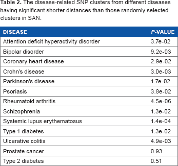
In the SAN, there are a number of nodes that correspond to known disease-related SNPs. Our results show that the distance distribution between SNP cluster nodes related to the same disease is significantly smaller than that from randomly selected nodes (Table 2). We have checked 13 different types of diseases (each with more than 20 nodes in the SAN). Eleven diseases showed significantly shorter distances between nodes while comparing with the random background (t-test, P < 0.05), with two diseases (prostate cancer, Type 2 diabetes) as exceptions. The smaller distances in SAN are also found in nodes that are related to the similar subtypes of diseases. Autoimmune diseases are caused by inappropriate immune responses of the body against substances and tissues normally present in the body.⁴² It has been shown that different autoimmune diseases are likely to share etiological similarities and underlying mechanisms.⁴³ In the SAN, 251 nodes are related to different subtypes of autoimmune diseases. Compared with the random background, the nodes related to the same subtype of disease form a more closely connected subnetwork. In the autoimmune-disease-related subnetwork, there are 183 edges and the size of the maximally connected subgraph is 64 (Fig. 4A), while in the random background the average number of edges is only 92 and the average size is 20 (both P-value = 0 by random sampling).

Figure 4.

(A) The maximally connected SAN subnetwork related to autoimmune diseases. Different colors mean different autoimmune diseases. SNP clusters in red contain SNPs related to multiple autoimmune diseases. (B) Quasi-clique QC1 (right) and its closely connected neighbors (left) that have connections with more than four nodes in QC1. Red: autoimmune-disease related. Yellow: others. (C) Quasi-clique QC2 (right) and its closely connected neighbors (left) that have connections with more than four nodes in QC2. Red: autoimmune-disease-related. Yellow: others.

Table 2.

The disease-related SNP clusters from different diseases having significant shorter distances than those randomly selected clusters in SAN.

DISEASE	P-VALUE
Attention deficit hyperactivity disorder	3.7e-02
Bipolar disorder	9.2e-03
Coronary heart disease	2.9e-02
Crohn's disease	3.0e-03
Parkinson's disease	1.7e-02
Psoriasis	3.8e-02
Rheumatoid arthritis	4.5e-06
Schizophrenia	1.3e-02
Systemic lupus erythematosus	1.4e-04
Type 1 diabetes	1.3e-02
Ulcerative colitis	4.9e-03
Prostate cancer	0.93
Type 2 diabetes	0.51

As the closely connected subnetworks in the SAN are likely associated with the same disease or phenotype, we can use the topological information of the SAN, such as the clustering coefficient and the shortest distance between nodes, to discover the potential high-order SNP combinations that are relevant to a disease or phenotype. For example, we examined the autoimmune-disease-related subnetwork and found two quasi-cliques (QC1 and QC2) that are separately comprised of eight nodes with 25 edges (Fig. 4B) and eight nodes with 24 edges (Fig. 4C). Studies had shown that these closely linked nodes in both cliques are related to autoimmune diseases. Thus, we inferred that the SAN nodes that have a close connection with nodes in QC1 and QC2 are also involved in autoimmune diseases. There are 7 and 33 SNP cluster nodes in SAN, respectively, that have direct connections with over one-half of the nodes in QC1 or QC2 (the SNP cluster nodes that are already in the autoimmune-disease-related subnetwork are excluded). For those seven SNP cluster nodes connected with QC1, there exist 12 genes of which 10 have been proven to be correlated to autoimmune diseases (P = 1.80 × 10⁻¹¹, binomial test). For example, STAT3 has been found to be essential for the differentiation of TH17 helper T cells in a variety of autoimmune diseases,⁴⁴ while, of those 33 SNP cluster nodes connected with QC2, 17 of 33 genes are proven to have a relationship with autoimmune diseases (P = 2.56 × 10⁻¹³, binomial test), such as CTSL1 and HLA-DQA1.^45,46

Prediction of Novel Disease-Related SNPs Based on the SNP Association Network

Guilt by association (GBA) is a proven approach for identifying novel disease genes based on the simple idea that genes that are associated with or interacting in a GIN are more likely to be associated with similar traits.^47,48 Similar to that of GIN, the genomic locus in the SAN, which has dense connections with the genomic loci that are proven to be related to certain diseases, is probably associated with this disease too. Therefore, we can explore known data of disease-related SNPs and the SAN topological structure to predict novel disease-related SNPs, with no need for introducing a new GWAS dataset. Based on the RWR strategy,²⁴ we developed a prediction algorithm by using the known disease-related genomic loci as seeds to predict new disease-related SNP cluster candidates. RWR is a ranking algorithm that simulates a random walker of proceeding coequally from each known disease-related seed node and then moving forward randomly to the immediate neighbors at each step. Meanwhile, the random walker can return at a probability “r” to the original seed nodes at each step. Thus, after several rounds of steps, the random walking will reach a steady state. All the nodes in the graph are then ranked by the probability of the random walker reaching the destination, which will evaluate the closeness between these nodes and the known disease-related seed nodes.

We tested our method (RWR-SAN) on known lung-cancer-related SNPs collected from the GWAS Catalog and the Lung Cancer Database.^23,49 For comparison, we also implemented a similar RWR procedure on the HPRD network (RWR-HPRD). In the SAN, the known lung-cancer-related SNPs were mapped into the corresponding SNP clusters, which are marked as disease-related nodes. In the HPRD network, these known lung-cancer-related SNPs were mapped into the nearest genes in the genome and also marked as disease-related nodes. We then used leave-one-out cross-validation to examine how well these algorithms recover the disease-related nodes. In each round of cross-validation, we selected one of the known disease-related nodes and used the rest of them as seed nodes. The held-out node and other 99 randomly picked nodes were ranked by the RWR algorithm. Here, we used the receiver operating characteristic (ROC) analysis to compare the two algorithms.⁵⁰ Sensitivity is the frequency of a disease-related node that was ranked above a particular threshold. Specificity is the frequency of a non-disease-related node ranked below this threshold. In order to compare different curves obtained by ROC analysis, we calculated the area under the ROC curve (AUC) for each case. As shown in Figure 5, the AUC value of RWR-SAN is much higher than that of RWR-HPRD (0.81 vs 0.66), which indicates that the prediction capability of RWR-SAN is much better than that of RWR-HPRD.

Figure 5.

ROC curves of RWR-SAN and RWR-HPRD in lung cancer data.

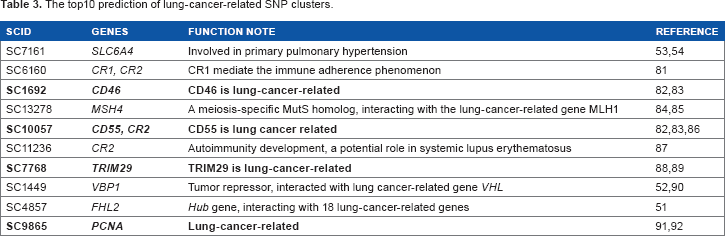
We further applied RWR-SAN to predict novel lung-cancer-related SNP clusters. All known lung-cancer-related nodes are treated as seed nodes to run RWR-SAN. For the top10 predicted SNP clusters (Table 3), four genomic loci had been proven to contain genes related to lung cancer and the other six loci also have reported evidences related to lung cancer. For instance, the gene FHL2 on SC4857⁵¹ is a hub gene in the HPRD that has interactions with other 39 genes. Among them, 18 have been related to lung cancer. Another example is the tumor suppressor gene VBP1 on SC1449, which has direct protein-protein interaction with VHL, another known lung-cancer gene.⁵² A more interesting example is the gene SLC6A4 on SC7161, which is involved in primary pulmonary hypertension (PPH).^53,54 Recent studies have shown that the genesis and progression of PPH is likely consistent with the model of tumorigenesis.^55,56

Table 3.

The top10 prediction of lung-cancer-related SNP clusters.

SCID	GENES	FUNCTION NOTE	REFERENCES
SC7161	SLC6A4	Involved in primary pulmonary hypertension	53,54
SC6160	CR1, CR2	CR1 mediate the immune adherence phenomenon	81
SC1692	CD46	CD46 is lung-cancer-related	82,83
SC13278	MSH4	A meiosis-specific MutS homolog, interacting with the lung-cancer-related gene MLH1	84,85
SC10057	CD55, CR2	CD55 is lung cancer related	82,83,86
SC11236	CR2	Autoimmunity development, a potential role in systemic lupus erythematosus	87
SC7768	TRIM29	TRIM29 is lung-cancer-related	88,89
SC1449	VBP1	Tumor repressor, interacted with lung cancer-related gene VHL	52,90
SC4857	FHL2	Hub gene, interacting with 18 lung-cancer-related genes	51
SC9865	PCNA	Lung-cancer-related	91,92

SAN-Assisted Reanalysis of an Age-Related Macular Degeneration GWAS Dataset

The topological information in SAN can be used as an external information source to assist GWAS data analysis. Borrowing from the Google's PageRank algorithm, we can reanalyze the GWAS dataset by integrating the typical GWAS data analysis method with the topological information in the SAN. We tested the performance of our SAN-assisted reanalysis on an AMD GWAS dataset.²⁵ Here, we adopted the iterative ranking method (details in Method section), in which a SNP cluster's score is calculated from an initial score (which is from typical GWAS analysis) and the normalized scores of its neighbors (which are iteratively updated).⁵⁷ According to our reanalysis, each SNP cluster receives a revised score with contributions from both direct evidence from the typical GWAS analysis and indirect evidence from the neighbors in the SAN. Then, we can rerank the SNP clusters based on their revised scores; the higher the rank of the SNP cluster, the closer its correlation with AMD.

In the GWAS analysis of the AMD dataset, Klein et al. found only one significant SNP, rs380390.²⁵ In our SAN-assisted reanalysis, SNP cluster SC7581 corresponds to SNP rs380390 and is still on the top of the list. Compared with the ranking by using the initial scores from GWAS analysis, the ranks of some SNP clusters get a significant boost after integrating the topological information of SAN (Table 4). For instance, there are two SNP clusters, SC9345 and SC962, whose ranks go up dramatically, with a jump from 541 in the original order to 2 in the reanalysis order for SC9345, and from 244 to 6 for SC962. AMD usually affects older adults and results in a loss of vision in the center of the macula because of damage to the retina.⁵⁸ The genomic region of SC9345 contains two genes, bHLHE41 and SSPN. bHLHE41 is the member of basic helix-loop-helix (bHLH) transcription factor family, which makes important contributions to the control of the proliferation and development during differentiation, particularly in neurons.^59–61 Studies employed in diverse experimental systems from various species have shown that bHLH genes play decisive roles in the generation of the diverse cell types during the development of the retina.^62–64 The gene on genomic locus of SC962 is CDH18, which belongs to CDH gene family, a family of calcium-dependent cell-cell adhesion molecules.^65,66 CDH genes mediate neural cell-cell interactions and may play important roles in neural development. For example, CDH3, a member of CDH family, had been proven to be associated with ectodermal dysplasia, ectrodactyly, and macular dystrophy (EEM syndrome).⁶⁷ Another member of CDH family, CDH8, has been also found related to retinal survival/protection.⁶⁸ More interestingly, in our SAN-assisted reanalysis, the rank of SNP cluster SC688, which contains the gene CDH8, is also boosted greatly, from rank 171 to rank 12. These results indicate that the reanalysis of GWAS data with our SAN may identify more potential disease-associated genes.

Table 4.

The reranking of top10 SNP clusters of the AMD GWAS dataset.

SCID	GENES	RANK_NEW	RANK_OLD
SC7581	CFHR3, CFH	1	1
SC9345	BHLHE41, SSPN	2	541
SC10154	SGCD	3	18
SC3466	VAC14	4	6
SC1673	TRPC4	5	7
SC962	CDH18	6	244
SC11017	TCF7L2	7	10
SC12214	C2ORF88, PMS1	8	2
SC1004	SGCZ	9	24
SC9695	ANKS1B	10	3

Discussion

So far, large-scale GWAS studies have produced massive data; therefore, how to further reanalyze these data has become an important issue. One reanalysis strategy of GWAS data is meta-analysis, which was originally developed for pooling the results from a set of similar clinical trials but is now widely used to combine different types of studies.^69–71 Another strategy is to introduce new information into GWAS data analysis to improve the detection power. It is very attractive to combine GWAS data with gene-interaction information, because the latter can provide us some hints on how to measure the association between SNPs. In this work, we established a general framework to integrate different sources of gene-interaction information to measure the association between SNPs. Although we only used the HPRD network as data resource in this work, our method is capable of integrating different types of gene-interaction information. By using gene-interaction data from different sources (such as protein interaction data, gene coexpression data), our SAN network can investigate SNPs’ correlation in different aspects. Systematically integrating SANs constructed from multiple data sources will allow us to obtain better effect on SAN-based prediction.

Over the last decade, GWAS have revealed a large number of disease- or trait-predisposing SNPs, but most of them are located within noncoding regions.⁷² Besides being the regulatory regions in a coding gene (such as enhancer), these SNPs are likely associated with some functional noncoding RNAs. For instance, there are two coronary-artery-diseases-related long noncoding RNAs, myocardial-infarction-associated transcript (MIAT), and antisense noncoding RNA in the INK4 locus (ANRIL) found in GWAS.⁷³ Recently, a database, named lncRNASNP, also collected such lncRNA-related SNPs, and found that 142 human lncRNA-related SNPs are GWAS-tag SNPs and 197,827 lncRNA-related SNPs are in the GWAS LD regions.⁷⁴ In our SAN, we studied only the coding region in the genome. But, if we exploit the coding-noncoding gene interaction/coexpression network into our SAN,⁷⁵ it can be further extended to SNPs-tagged noncoding region and be used to annotate lncRNA-related SNP's function.

The studies of SAN can not only perform auxiliary GWAS analysis but also offer biologically meaningful information by itself. In the known studies on GINs, network topology provided important information for function study, and a lot of tools mining functional module were applied greatly to accelerate protein function prediction.⁷⁶⁻⁷⁸ As to how to apply our SAN network structure, here we made a preliminary attempt, including analysis of autoimmune-disease-related quasi-cliques and the RWR method in SAN. Instead of inspecting the possible distinctions between SAN and known gene-interaction networks, we directly used algorithms developed in GIN study. It is believed that by combining the numerous disease-related SNPs in GWASs with in-depth studies of specific characteristics of the SAN network structure, our SAN study can further assist in the prediction of potential disease-related chromosome regions and allow us to find the possible interactions between different diseases.

Methods

SNP Association Score

As shown in Formula 1, the SAS between each pair of SNP_i and SNP_j is calculated based on the connectivity among genes inside of the loci. G_i/G_j represents a gene set in chromosomal region of SNP_i/SNP_j, respectively. A GIN is any interaction/association network between genes. In this work, we use HPRD network.²⁹ D_GIN is a scoring function of gene association based on GIN; here we use the diffusion kernel matrix of HPRD network.²⁸

S A S (S N P_{i}, S N P_{j}) = f (G_{i}, G_{j}, G I N) = \sum_{g \in G i} \sum_{g' \in G j} D_{G I N} (g, g')

(1)

Diffusion Kernel on Graph

As shown in Formula 2, diffusion kernel of a graph G is a matrix exponential, where k_ij measures the similarity between nodes v_i and v_j.²⁸ The matrix L is the Laplacian of the graph G, defined as E–D, where E is the adjacency matrix and D is a diagonal matrix containing the nodes’ degrees. The real parameter β controls the magnitude of the diffusion, and its optimal value is data-dependent.

Diffusion kernel on graph is a global measure of similarity since it is calculated using the global connectivity information (ie, adjacency and degree information). In addition, compared with another common measure, namely the shortest path distance similarity that is extremely sensitive to random insertion/deletion of edges, diffusion kernel is more robust to deal with extensive noise in high-throughput datasets.⁷⁹

D_{G I N} (g, g') = K = (k a b) = e^{β L_{a b}}, a, b = 1, 2, \dots, n

(2)

Empirical P-Value of sAs

For each SNP cluster pair (i, j) and its SAS_i,j, we can compute its corresponding empirical P-value by Formula 3. BKG is the background set of SNP cluster pairs that are generated by randomly picking two SNP clusters that have the same numbers of genes in their neighborhoods, and these genes have the same degrees in the HPRD network. μ(SAS_BKG) is the mean value of all SASs in the set BKG, and σ(SAS_BKG) is the standard deviation of all SASs in the set BKG.

p v a l u e (S A S_{i, j}) = p n o r m (- a b s (\frac{S A S_{i, j} - μ (S A S_{B K G})}{σ (S A S_{B K G})}))

(3)

Random Walk with Restart

RWR is a ranking algorithm that simulates a random walker who starts on a set of seed nodes and iteratively transits from its current node to a randomly selected immediate neighbor. At each step, the random walker can return to the seed nodes with a certain restart probability. Finally, all the nodes in the graph are ranked by the probability of the random walker reaching this node.²⁴

RWR can be formally defined as Formula 4. The parameter gamma ∊ (0, 1) is the restart probability (in our application it is set as 0.5). The transition matrix W is the column-normalized adjacency matrix of the graph, and W_ij is the transition probability from node i to node j. P₀ is the initial probability vector, which was constructed such that equal probabilities were assigned to the seed nodes with the sum of the probabilities equal to 1. P_t is a vector in which the ith element holds the probability of finding the random walker at node i at step t.

After some steps, the probability vector will reach a steady state P_∞, which gives a measure of proximity to seed nodes. If P_∞(i) > P_∞(j), then node i is more proximate to seed nodes than node j. This is obtained by performing the iteration until the difference between P_t and P_t₊₁ (measured by the L1 norm) fall below 10⁻¹⁰.

P_{t + 1} = (1 - g a m m a) \times W \times P_{t} + g a m m a \times P_{0}

(4)

SAN-Assisted GWAS re-analysis

SAN-assisted GWAS reanalysis computes a score S_C for each SNP cluster C. The higher the score, the closer will be its correlation with diseases or traits. First, by Formula 5 in which Φ⁻¹ is the inverse cumulative distribution function (CDF) of normal distribution, all SNPs’ P-values from the original GWAS study will be transferred to z-scores; that is, smaller P-values correspond to larger z-scores.⁸⁰ Second, each SNP-cluster's score S_C will be initialized as O_C, which is the maximum z-score of all SNPs covered. Then, each SNP-cluster's score S_C will be iteratively updated by adding the average score of its immediate neighbors according to Formula 6, where NB(C) is the set of immediate neighboring nodes of the SNP cluster C.⁵⁷ The parameter (1 – gamma)/gamma weights the network's contribution to the reanalysis score. Previous work⁵⁷ has proved that this iterative ranking method can converge to a unique solution very fast and is not sensitive to the range of (1 – gamma)/gamma.^5,50 Here, we set it as 5 in our application.

z_{i} = Φ^{- 1} (1 - p i)

(5)

S_{C}^{(t + 1)} = O_{C} \times g a m m a + \underset{N \in N B (C)}{A V G} (S_{N}^{(t)}) \times (1 - g a m m a)

(6)

Data Sources

Human SNP dataset: UCSC Genome Browser (genome.ucsc.edu, SNP132_common). HPRD network: Human Protein Reference Database (www.hprd.org, date 2011–4).

Disease-related SNPs: NIH GWAS catalog (www.genome.gov/gwastudies, date 2011–6).

HapMap genotype dataset: HapMap (hapmap.ncbi.nlm.nih.gov, date 2011–11).

HiC dataset: Hi-C Data Browser (hic.umassmed.edu).

Lung cancer database: HLungDB (www.megabionet.org/bio/hlung).

Coronary heart disease database: CADgene (www.bioguo.org/CADgene).

Prostate cancer database: DDPC (www.cbrc.kaust.edu.sa/ddpc).

Schizophrenia database: SZGR (bioinfo.vipbg.vcu.edu: 8080/SZGR).

Author Contributions

Conceived and designed the experiments: CL, ZX. Analyzed the data: CL. Wrote the first draft of the manuscript: CL. Agree with manuscript results and conclusions: CL, ZX. Jointly developed the structure and arguments for the paper: CL, ZX. Made critical revisions and approved final version: CL, ZX. Both authors reviewed and approved of the final manuscript.

References

Hirschhorn

J.N.

, Daly

M.J.

Genome-wide association studies for common diseases and complex traits. Nat Rev Genet. Fire extinguisher(Powder) 2005; 6: 95–108.

Wang

W.Y.

, Barratt

B.J.

, Clayton

D.G.

, Todd

J.A.

Genome-wide association studies: theoretical and practical concerns. Nat Rev Genet. 2005; 6: 109–18.

Rioux

J.D.

, Xavier

R.J.

, Taylor

K.D.

Genome-wide association study identifies new susceptibility loci for Crohn disease and implicates autophagy in disease pathogenesis. Nat Genet. 2007; 39: 596–604.

Zanke

B.W.

, Greenwood

C.M.

, Rangrej

Genome-wide association scan identifies a colorectal cancer susceptibility locus on chromosome 8q24. Nat Genet. 2007; 39: 989–94.

Garcia-Closas

, Couch

F.J.

, Lindstrom

; Familial Breast Cancer Study (FBCS); Australian Breast Cancer Tissue Bank (ABCTB) Investigators. Genome-wide association studies identify four ER negative-specific breast cancer risk loci. Nat Genet. 2013; 45(4): e391–2.

, Wang

, Song

Joint analysis of three genome-wide association studies of esophageal squamous cell carcinoma in Chinese populations. Nat Genet. 2014; 46(9): 1001–6.

Williams

S.M.

, Canter

J.A.

, Crawford

D.C.

, Moore

J.H.

, Ritchie

M.D.

, Haines

J.L.

Problems with genome-wide association studies. Science. 2007; 316: 1840–2.

Visscher

P.M.

, Brown

M.A.

, Yang

Five years of GWAS discovery. The American Journal of Human Genetics. 2012; 90: 7–24.

Amos

C.I.

Successful design and conduct of genome-wide association studies. Hum Mol Genet. 2007; 16: R220–5.

10.

McCarthy

M.I.

, Abecasis

G.R.

, Cardon

L.R.

Genome-wide association studies for complex traits: consensus, uncertainty and challenges. Nat Rev Genet. 2008; 9: 356–69.

11.

Frazer

K.A.

, Murray

S.S.

, Schork

N.J.

, Topol

E.J.

Human genetic variation and its contribution to complex traits. Nat Rev Genet. 2009; 10(4): 241–51.

12.

Manolio

T.A.

, Collins

F.S.

, Cox

N.J.

Finding the missing heritability of complex diseases. Nature. 2009; 461: 747–53.

13.

Eichler

E.E.

, Flint

, Gibson

Missing heritability and strategies for finding the underlying causes of complex disease. Nat Rev Genet. 2010; 11: 446.

14.

Marchini

, Donnelly

, Cardon

L.R.

Genome-wide strategies for detecting multiple loci that influence complex diseases. Nat Genet. 2005; 37: 413–7.

15.

, Bush

W.S.

, Moore

J.H.

Bioinformatics challenges for genome-wide association studies. Bioinformatics. 26. 2010; 4: 445–55.

16.

Neale

B.M.

, Sham

P.C.

The future of association studies: gene-based analysis and replication. Am J Hum Genet. 2004; 75: 353–62.

17.

Wang

, Li

, Bucan

Pathway-based approaches for analysis of genome-wide association studies. Am J Hum Genet. 2007; 81: 1278–83.

18.

Chen

, Cho

, Zhao

Incorporating biological pathways via a Markov random field model in genome-wide association studies. PLoS Genet. 2011; 7(4): e1001353.

19.

Lee

, Blom

U.M.

, Wang

P.I.

, Shim

J.E.

, Marcotte

E.M.

Prioritizing candidate disease genes by network-based boosting of genome-wide association data. Genome Res. 2011; 21: 1109–21.

20.

Hou

, Chen

, Zhang

C.K.

, Cho

, Zhao

Guilt by rewiring: gene prioritization through network rewiring in genome wide association studies. Hum Mol Genet. 2014; 23(10): 2780–90.

21.

Altshuler

D.M.

, Gibbs

R.A.

, Peltonen

; International HapMap 3 Consortium. Integrating common and rare genetic variation in diverse human populations. Nature. 2010; 467: 52–8.

22.

Lieberman-Aiden

, van Berkum

N.L.

, Williams

Comprehensive mapping of long-range interactions reveals folding principles of the human genome. Science. 2009; 326: 289–93.

23.

Welter

, MacArthur

, Morales

The NHGRI GWAS Catalog, a curated resource of SNP-trait associations. Nucleic Acids Res. 2014; 42(Database issue): D1001–6.

24.

Köhler

, Bauer

, Horn

, Robinson

P.N.

Walking the interactome for prioritization of candidate disease genes. Am J Hum Genet. 2008; 82: 949–58.

25.

Klein

R.J.

, Zeiss

, Chew

E.Y.

Complement factor H polymorphism in age-related macular degeneration. Science. 2005; 308: 385–9.

26.

Lewis

C.M.

, Knight

Introduction to genetic association studies. Cold Spring Harb Protoc. 2012; 3: 297–306.

27.

Barabasi

A.L.

, Gulbahce

, Loscalzo

Network medicine: a network-based approach to human disease. Nat Rev Genet. 2011; 12(1): 56–68.

28.

Kondor

R.I.

, Lafferty

Morgan Kaufmann Publishers Inc. San Francisco, CA, USA. Diffusion Kernels on Graphs and Other Discrete Input Spaces: Proceeding ICML'02 Proceedings of the Nineteenth International Conference on Machine Learning; 2002; 315–22.

29.

Keshava Prasad

T.S.

, Goel

, Kandasamy

Human protein reference database – 2009 update. Nucleic Acids Res. 2009; 37: D767–72.

30.

Barabási

A.L.

Scale-free networks: a decade and beyond. Science. 2009; 325(5939): 412–3.

31.

Krzywinski

, Schein

, Birol

Circos: an information aesthetic for comparative genomics. Genome Res. 2009; 19: 1639–45.

32.

Hill

W.G.

Estimation of linkage disequilibrium in randomly mating populations. Heredity. 1974; 33: 229.

33.

Agarwala

, Sanders

T.A.

, Ragsdale

C.W.

Sonic hedgehog control of size and shape in midbrain pattern formation. Science. 2001; 291: 2147–50.

34.

Bénazet

J.D.

, Bischofberger

, Tiecke

A self-regulatory system of interlinked signaling feedback loops controls mouse limb patterning. Science. 2009; 323: 1050–3.

35.

Bale

A.E.

, Yu

K.P.

The hedgehog pathway and basal cell carcinomas. Hum Molec Genet. 2001; 10: 757–62.

36.

Berman

D.M.

, Karhadkar

S.S.

, Maitra

Widespread requirement for hedgehog ligand stimulation in growth of digestive tract tumours. Nature. 2003; 425: 846–51.

37.

Villavicencio

E.H.

, Walterhouse

D.O.

, Iannaccone

P.M.

The sonic hedgehog–patched–gli pathway in human development and disease. Am J Hum Genet. 2000; 67: 1047–54.

38.

Katoh

, Katoh

Hedgehog signaling, epithelial-to-mesenchymal transition and miRNA. Int J Mol Med. 2008; 22(3): 271–5.

39.

Villavicencio

E.H.

, Yoon

J.W.

, Frank

D.J.

, Füchtbauer

E.M.

, Walterhouse

D.O.

, Iannaccone

P.M.

Cooperative E-box regulation of human GLI1 by TWIST and USF. Genesis. 2002; 32(4): 247–58.

40.

el Ghouzzi

, Le Merrer

, Perrin-Schmitt

Mutations of the TWIST gene in the Saethre-Chotzen syndrome. Nat Genet. 1997; 15(1): 42–6.

41.

El Ghouzzi

, Legeai-Mallet

, Aresta

Saethre-Chotzen mu-tations cause TWIST protein degradation or impaired nu-clear location. Hum Mol Genet. 2000; 9: 813–9.

42.

Rose

N.R.

, Bona

Defining criteria for autoimmune diseases. Immunol Today. 1993; 14(9): 426–30.

43.

Davidson

, Diamond

Autoimmune diseases. N Engl J Med. 2001; 345: 340–50.

44.

Chaudhry

, Rudra

, Treuting

CD4(+) regulatory T cells control TH17 responses in a Stat3-dependent manner. Science. 2009; 326: 986–91.

45.

Maehr

, Mintern

J.D.

, Herman

A.E.

Cathepsin L is essential for onset of autoimmune diabetes in NOD mice. J Clin Invest. 2005; 115: 2934–43.

46.

Wallaschofski

, Meyer

, Tuschy

, Lohmann

HLA-DQA1*0301-associated susceptibility for autoimmune polyglandular syndrome type II and III. Horm Metab Res. 2003; 35(2): 120–4.

47.

Oliver

Guilt-by-association goes global. Nature. 2000; 403(6770): 601–3.

48.

Ideker

, Sharan

Protein networks in disease. Genome Res. 2008; 18: 644–52.

49.

Wang

, Xiong

, Sun

HLungDB: an integrated database of human lung cancer research. Nucleic Acids Res. 2010; 38(Database issue): D665–9.

50.

Aerts

, Lambrechts

, Maity

Gene prioritization through genomic data fusion. Nat Biotechnol. 2006; 24: 537–44.

51.

Chan

K.K.

, Tsui

S.K.

, Lee

S.M.

Molecular cloning and characterization of FHL2, a novel LIM domain protein preferentially expressed in human heart. Gene. 1998; 210: 345–50.

52.

Miyakis

, Liloglou

, Kearney

, Xinarianos

, Spandidos

D.A.

, Field

J.K.

Absence of mutations in the VHL gene but frequent loss of heterozygosity at 3p25–26 in non-small cell lung carcinomas. Lung Cancer. 2003; 39(3): 273–7.

53.

Eddahibi

, Humbert

, Fadel

Serotonin transporter overexpression is responsible for pulmonary artery smooth muscle hyperplasia in primary pulmonary hypertension. J Clin Invest. 2001; 108: 1141–50.

54.

Eddahibi

, Chaouat

, Morrell

Polymorphism of the serotonin transporter gene and pulmonary hypertension in chronic obstructive pulmonary disease. Circulation. 2003; 108: 1839–44.

55.

Voelkel

N.F.

, Cool

, Lee

S.D.

, Wright

, Geraci

M.W.

, Tuder

R.M.

Primary pulmonary hypertension between inflammation and cancer. Chest. 1998; 114: 225S–30.

56.

Rai

P.R.

, Cool

C.D.

, King

J.A.

The cancer paradigm of severe pulmonary arterial hypertension. Am J Respir Crit Care Med. 2008; 178: 558–64.

57.

Ramakrishnan

S.R.

, Vogel

, Kwon

, Penalva

L.O.

, Marcotte

E.M.

, Miranker

D.P.

Mining gene functional networks to improve mass-spectrometry-based protein identification. Bioinformatics. 2009; 25: 2955–61.

58.

Tuo

, Bojanowski

C.M.

, Chan

C.C.

Genetic factors of age-related macular degeneration. Prog Retin Eye Res. 2004; 23(2): 229–49.

59.

Lee

J.E.

Basic helix-loop-helix genes in neural development. Curr Opin Neurobiol. 1997; 7: 13–20.

60.

Kageyama

, Ishibashi

, Takebayashi

, Tomita

bHLH transcription factors and mammalian neuronal differentiation. Int J Biochem Cell Biol. 1997; 29(12): 1389–99.

61.

Ledent

, Vervoort

The basic helix-loop-helix protein family: comparative genomics and phylogenetic analysis. Genome Res. 2001; 11: 754–770.

62.

Hatakeyama

, Kageyama

Retinal cell fate determination and bHLH factors. Semin Cell Dev Biol. 2004; 15(1): 83–9.

63.

Wang

J.C.

, Harris

W.A.

The role of combinational coding by homeodomain and bHLH transcription factors in retinal cell fate specification. Dev Biol. 2005; 285(1): 101–15.

64.

Yan

R.T.

, Ma

, Liang

, Wang

S.Z.

bHLH genes and retinal cell fate specification. Mol Neurobiol. 2005; 32(2): 157–71.

65.

Hirano

, Nose

, Hatta

, Kawakami

, Takeichi

Calcium-dependent cell-cell adhesion molecules (cadherins): subclass specificities and possible involvement of actin bundles. J Cell Biol. 1987; 105(6 pt 1): 2501–10.

66.

Takeichi

The cadherins: cell-cell adhesion molecules controlling animal morphogenesis. Development. 1988; 102: 639–55.

67.

Kjaer

K.W.

, Hansen

, Schwabe

G.C.

Distinct CDH3 mutations cause ectodermal dysplasia, ectrodactyly, macular dystrophy (EEM syndrome). J Med Genet. 2005; 42(4): 292–8.

68.

Cai

, Fields

M.A.

, Hoshino

, Priore

L.V.

Effects of aging and anatomic location on gene expression in human retina. Front Aging Neurosci. 2012; 4: 8.

69.

Thompson

J.R.

, Attia

, Minelli

The meta-analysis of genome-wide association studies. Brief Bioinform. 2011; 12(3): 259–69.

70.

Springelkamp

, Höhn

, Mishra

Meta-analysis of genome-wide association studies identifies novel loci that influence cupping and the glaucomatous process. Nat Commun. 2014; 5: 4883.

71.

Woo

, Falcone

G.J.

, Devan

W.J.

; International Stroke Genetics Consortium. Meta-analysis of genome-wide association studies identifies 1q22 as a susceptibility locus for intracerebral hemorrhage. Am J Hum Genet. 2014; 94(4): 511–21.

72.

Hindorff

L.A.

, Sethupathy

, Junkins

H.A.

Potential etiologic and functional implications of genome-wide association loci for human diseases and traits. Proc Natl Acad Sci USA. 2009; 106: 9362–7.

73.

, Xuan

, Liu

Long non-coding RNAs and complex human diseases. Int J Mol Sci. 2013; 14(9): 18790–808.

74.

Gong

, Liu

, Zhang

, Miao

, Guo

A.Y.

lncRNASNP: a database of SNPs in lncRNAs and their potential functions in human and mouse. Nucl Acids Res. 2014; 43(Database issue): D181–6.

75.

Liao

, Liu

, Yuan

Large-scale prediction of long non-coding RNA functions in a coding-non-coding gene co-expression network. Nucl Acids Res. 2011; 39(9): 3864–78.

76.

Bader

G.D.

, Hogue

C.W.

An automated method for finding molecular complexes in large protein interaction networks. BMC Bioinformatics. 2003; 4: 2.

77.

Adamcsek

, Palla

, Farkas

I.J.

, Derényi

, Vicsek

CFinder: locating cliques and overlapping modules in biological networks. Bioinformatics. 2006; 22: 1021–3.

78.

Liu

, Li

, Zhao

Exploring hierarchical and overlapping modular structure in the yeast protein interaction network. BMC Genomics. 2010; 11(suppl 4): S17.

79.

Kondor

, Vert

J.P.

Diffusion kernels. In: Scholkopf

, Tsuda

, Vert

J.P.

eds. Kernel Methods in Computational Biology. Cambridge, MA: The MIT Press; 2004: 400.

80.

Ideker

, Ozier

, Schwikowski

, Siegel

A.F.

Discovering regulatory and signalling circuits in molecular interaction networks. Bioinformatics. 2002; 18(suppl 1): S233–40.

81.

Smith

B.O.

, Mallin

R.L.

, Krych-Goldberg

Structure of the C3b binding site of CR1 (CD35), the immune adherence receptor. Cell. 2002; 108: 769–80.

82.

Varsano

, Frolkis

, Ophir

Expression and distribution of cell-membrane complement regulatory glycoproteins along the human respiratory tract. Am J Respir Crit Care Med. 1995; 152(3): 1087–93.

83.

Varsano

, Rashkovsky

, Shapiro

, Ophir

, Mark-Bentankur

Human lung cancer cell lines express cell membrane complement inhibitory proteins and are extremely resistant to complement-mediated lysis; a comparison with normal human respiratory epithelium in vitro, and an insight into mechanism(s) of resistance. Clin Exp Immunol. 1998; 113(2): 173–82.

84.

Paquis-Flucklinger

, Santucci-Darmanin

, Paul

, Saunieres

, Turc-Carel

, Desnuelle

Cloning and expression analysis of a meiosis-specific MutS homolog: the human MSH4 gene. Genomics. 1997; 44: 188–94.

85.

Hsu

H.S.

, Wen

C.K.

, Tang

Y.A.

Promoter hypermethylation is the predominant mechanism in hMLH1 and hMSH2 deregulation and is a poor prognostic factor in nonsmoking lung cancer. Clin Cancer Res. 2005; 11(15): 5410–6.

86.

Varsano

, Rashkovsky

, Shapiro

, Radnay

Cytokines modulate expression of cell-membrane complement inhibitory proteins in human lung cancer cell lines. Am J Respir Cell Mol Biol. 1998; 19(3): 522–9.

87.

Asokan

, Hua

, Young

K.A.

Characterization of human complement receptor type 2 (CR2/CD21) as a receptor for IFN-alpha: a potential role in systemic lupus erythematosus. J Immunol. 2006; 177: 383–94.

88.

Hawthorn

, Stein

, Panzarella

, Loewen

G.M.

, Baumann

Characterization of cell-type specific profiles in tissues and isolated cells from squamous cell carcinomas of the lung. Lung Cancer. 2006; 53(2): 129–42.

89.

Zhou

Z.Y.

, Yang

G.Y.

, Zhou

, Yu

M.H.

Significance of TRIM29 and beta-catenin expression in non-small-cell lung cancer. J Chin Med Assoc. 2012; 75(6): 269–74.

90.

Tsuchiya

, Iseda

, Hino

Identification of a novel protein (VBP-1) binding to the von Hippel-Lindau (VHL) tumor suppressor gene product. Cancer Res. 1996; 56: 2881–5.

91.

Ishida

, Kaneko

, Akazawa

, Tateishi

, Sugio

, Sugimachi

Proliferating cell nuclear antigen expression and argyrophilic nucleolar organizer regions as factors influencing prognosis of surgically treated lung cancer patients. Cancer Res. 1993; 53(20): 5000–3.

92.

Ogawa

, Tsurumi

, Yamada

, Koide

, Shohtsu

Blood vessel invasion and expression of sialyl Lewisx and proliferating cell nuclear antigen in stage I non-small cell lung cancer. Relation to postoperative recurrence. Cancer. 1994; 73(4): 1177–83.

Prioritization of Cancer-Related Genomic Variants by SNP Association Network

Abstract

Keywords

Introduction

Result

General Idea of SNP Association Network Construction

Parameter Setting for the SNP Association Network Construction

Linkage Disequilibrium of SNP Cluster Nodes in the SNP Association Network

HiCinteraction between SNP Cluster Nodes in the SNP Association Network

Close Correlation of Known Disease-Related SNP Cluster Nodes in the SNP Association Network

Prediction of Novel Disease-Related SNPs Based on the SNP Association Network

SAN-Assisted Reanalysis of an Age-Related Macular Degeneration GWAS Dataset

Discussion

Methods

SNP Association Score

Diffusion Kernel on Graph

Empirical P-Value of sAs

Random Walk with Restart

SAN-Assisted GWAS re-analysis

Data Sources

Author Contributions

References