Sage Journals: Discover world-class research

Abstract

Binary tree classification has been useful for classifying the whole population based on the levels of outcome variable that is associated with chosen predictors. Often we start a classification with a large number of candidate predictors, and each predictor takes a number of different cutoff values. Because of these types of multiplicity, binary tree classification method is subject to severe type I error probability. Nonetheless, there have not been many publications to address this issue. In this paper, we propose a binary tree classification method to control the probability to accept a predictor below certain level, say 5%.

Keywords

binary tree classification permutation single-step procedure step-down procedure type I error

Introduction

A classification tree is a rule for predicting the class of an object from the values of its predictors. A tree is built by recursively partitioning and splitting it up further on each of the branches. The first tree-structured approach was the Automatic Interaction Detection (AID) program.¹ In this program, recursive partitioning was used as an alternative to the least squares regression for model fitting. Breiman et al.² developed the Classification and Regression Trees (CART) method of selecting tree of appropriate size for classification and regression. CART, THAID,³ and C4.5⁴ search exhaustively for a split of a node by minimizing a measure of node heterogeneity. These methods may cause a selection bias, because variables with more distinct values have a higher chance to be chosen. Loh and Vanichsetakul⁵ proposed a Fast Algorithm for Classification Trees (FACT) by recursive application of linear discriminant analysis. Quick, Unbiased, Efficient Statistical Trees (QUEST)⁶ and Classification Rule with Unbiased Interaction Selection and Estimation (CRUISE)⁷ use similar approach to test for the split without an exhaustive search. CART and QUEST use binary split, while FACT, C4.5, CHAID,⁸ and FIRM⁹ use multiway split.

In a classification tree, each partition is represented by a node in the tree. The process starts with a training set with known classes or with a cross-validation. A node in a tree splits recursively with the goal of making the data within each node more homogeneous according to a splitting criterion until the tree is fully grown. A measure of node impurity given a node can be defined by the Gini diversity index.² For growing a large initial tree, the nodes continue splitting until a terminal node is either pure or it contains a small number of observations. Pruning is used to remove nodes and branches to avoid overfitting.

In CART, after the initial large tree is constructed, a nested sequence of subtrees is obtained by progressively deleting branches according to the pruning method. Breiman et al.² defined the cost-complexity measure by imposing penalty (complexity parameter) to the number of terminal nodes. To choose the best tree among the nested subtrees, they recommend estimating the optimal complexity parameter by minimizing the cross-validation or the holdout sample error. Besides cost-complexity pruning, various pruning algorithms including reduced-error pruning,¹⁰ minimum description length pruning,^11–13 and minimum error pruning¹⁴ have been developed.

There have been other works aiming at correcting the classification bias due to large number of candidate predictors in a more general context not restricted to the tree classification. Bernau et al.¹⁵ developed a bias-correction method based on a decomposition of the unconditional error rate of the tuning procedure. Tibshirani and Tibshirani¹⁶ proposed a biased correction method for the minimum value of the cross-validation error. Ding et al.¹⁷ introduced a biased correction method based on learning curve fitting by inverse power law.

In this paper, we propose to control the type I error accounting for the multiplicity due to many candidate predictors and possible cutoff values for each of them. Employing the family-wise error rate concept that is used for multiple testing, our type I error rate is defined as the probability to have at least one split when none of the candidate predictors are associated with the clinical outcome. We also propose two permutation-based procedures, called single-step procedure (SSP) and step-down procedure (SDP), to control the multiplicity-adjusted type I error. We perform extensive simulations to show that the two procedures control the type I error accurately and have reasonable power with moderate sample sizes. We apply the proposed methods to the classification with real microarray data. Through simulation and real data analysis, we observe that SDP tends to make larger trees than SSP.

Methods

Suppose that there are m splitting variables x = (x₁, …, x_m), also called candidate predictors, that are believed to predict a response variable y, also called clinical outcome. Each splitting variable may be discrete (ordered or categorical) or continuous, and different variables may have different types like typical predictors in clinical data. The response variable may be of any type, eg, binary, continuous, or censored survival variable. We consider binary classification tree partitioning the target dataset into two subsets defined by the values of each variable. If x_j is a binary variable, there exists only one possible classification by x_j. If x_j is a continuous or ordered discrete variable, then we can classify the current dataset by using each observed value of x_j in the current dataset. If x_j is a categorical (ie, nominal discrete) variable with K different categories in the current data set, then we can classify the current dataset into two subsets by $\sum_{k = 1}^{(k - 1) / 2} (_{k}^{K})$ different ways, if K(≫2) is odd, and $\sum_{k = 1}^{K / 2} (_{k}^{K})$ different ways, if K(≫2) is even.

Let R_j denote the set of all possible splitting points of the current dataset by the values of x_j. Note that R_j will be unchanged if x_j has never been chosen as the splitting variable at an intermediate node. As x_j is chosen as a splitting variable, R_j will get smaller for nodes in a lower level of the tree. Let Z_j_(c) and p_j_(c) denote the standardized test statistic and its P value, respectively, to test the null hypothesis that the distribution of the response variable is identical between two groups that are defined by a classification c ∊ R_j. If y is a binary variable, Z_j_(c) may be the χ² test statistic with one degree of freedom; if y is a continuous variable, Z_j_(c) may be the two-sample t-test or Wilcoxon rank sum test; if y is a censored variable, Z_j_(c) may be the log-rank test statistic. Note that the type of test statistics will be identical for all predictors since the test statistic is chosen by the type of y and not by the type of a predictor. We assume that a large value of the test statistic (or its absolute value) implies evidence against the null hypothesis.

In a binary classification tree, we will continue classifying each sub-sample if there exists any predictor with a splitting point classifying the current subset with a P-value smaller than ø, or equivalently with a standardized test statistic larger than ζ. We propose a false positivity control by maintaining the probability of splitting the original data below a certain level α under the null hypothesis H₀ that none of the m classifiers are associated with the response. Toward this aim, we want to find the critical values ø = ø _alpha; or ζ = ζ_α satisfying

α = P (\bar{p} \leq ϕ | H_{0}) = P (\bar{Z} \geq ζ | H_{0}),

(1) where

\bar{P} = \min_{1 \leq j \leq m} \min_{c \in {\bar{R}}_{j}} P_{j (c),} \bar{Z} = \max_{1 \leq j \leq m} \max_{c \in {\bar{R}}_{j}} Z_{j (c)},

and

{\bar{R}}_{j}

is the set of all possible partitioning methods by the values of x_j in the original data. We present two procedures to control the type I error rate at a specified level in a classification tree.

Single-step procedure

Once we have the significance level ø_α (or critical value ζ_α) in (1), we will continue the classification until we do not find any splitting variable whose P-value is smaller than ø_α (or whose test statistic is larger than ζ_α) for any possible cutoff value. Since we use the same critical value at each splitting, we call it an SSP.

Since the splitting variables as well as the test statistics (or the P-values) defined by different cutoff values of each splitting variable are complicatedly correlated, it is difficult to analytically derive the critical value ζ (or the significant level ø) by solving (1). Hence, we propose to estimate the critical values by simulating the null distribution of the P-values (or test statistics) using a permutation method.

Permutation Procedure for ø_α

Conduct the following process for B permutations.

At the bth (b = 1, …, B) permutation,

Randomly match response variables y₁, …, y_n with splitting variables x₁, …, x_m.

Calculate $\bar{Z}, {\bar{Ζ}}_{b}$ , from the permuted data.

Approximate ø_α by the [αB]th order statistic of ${\bar{p}}_{1}, …, {\bar{p}}_{B},$ where [a] denotes the largest integer not exceeding a. Permutation Procedure for ζ_α

At the bth (b = 1, …, B) permutation,

Randomly match y₁, …, y_n with predictors x₁, …, x_m.

Calculate $\bar{Z}, {\bar{z}}_{b},$ from the permuted data.

Approximate ζα by the [(1 - α)B]th order statistic of ${\bar{z}}_{1}, …, {\bar{z}}_{B} .$

We conduct B = 1,000 permutations in our simulations of Section 3 and in real data analysis of Section 4. The exact significance level ø_α and critical value ζ_α will depend on the dependency among the splitting variables. Note that above-mentioned permutation methods provide a significance level and a critical value accounting for the dependence structure.

When presenting a classification tree, we may want to show how significant the classification is for each node with a split. To this end, we propose to calculate the P-value adjusting for multiplicity as follows. For a node, let $\hat{ζ}$ and $\hat{ϕ}$ denote the maximum test statistic value and the corresponding P-value, respectively, with respect to all splitting variables and all possible cutoff values for each splitting variable from the current data set. Then, the adjusted P-value for the classification at this node is defined by

P - value = P (\bar{Z} \geq \hat{ζ} | H_{0}) = P (\bar{p} \leq \hat{ϕ} | H_{0}) .

An approximate P-value can be calculated by approximating the null distribution of $\bar{Z}$ or $\bar{p}$ using above-mentioned permutation method.

Step-down procedure

Although SSP is simple to implement, it may not have a high power to identify significant prognostic predictors since it applies the same strict critical value (or significance level) at all partitioning of subtrees that have smaller numbers of possible cutoff values than the original data. In this section, we propose a multistep procedure, called SDP, that is expected to discover more prognostic predictors than SSP while controlling the type I error rate α at the same level.

We define node l(= 0, 1, …) as the l-th node counting from the root node to subsequent levels. At the same level, counting goes from left to right. Let D₇ denote the subset of the original data included in node l. Under the null hypothesis H_l, we assume that none of the m classifiers are associated with the response in D_l. When partitioning node l, we obtain the significance level ø_l = ø_l,α and critical value ζ_l =_ζl,α for type I error rate α from

α = P ({\bar{p}}_{l} \leq ϕ_{l} | H_{l}) = P ({\bar{Z}}_{l} \geq ζ_{l} | H_{l}),

where ${\bar{P}}_{l} = \min_{1 \leq j \leq m} \min_{c \in R_{l j}} P_{j (c)}, {\bar{Z}}_{l} = \max_{1 \leq j \leq m} \max_{c \in R_{l j}} Z_{j (c)},$ and R_j. is the set of all possible splitting points by the values of x_j in the current data set D_l. We split the current node at the partitioning with the smallest P-value if it is smaller than ø_l,α or equivalent with the largest test statistic in absolute value if it is larger than ζ_l,α.

As the partitioning continues, the size of current data set for each node decreases and the statistical tests to determine a partition suffer less multiple testing burden, so that the critical values for SDP are less strict than those of SSP for the subtrees. Hence, SDP may grow a larger tree than SSP. The significance level ø_l = ø_l,α and critical value ζ _l = ζ_l,α can be estimated using a permutation method as follows.

Permutation procedure for ø_l,α

At node l (= 0, 1, …), we want to estimate the critical value and the significance level for determining a partition from the current data set D_l = {y_{i_k},x_{i_k}), k = 1, …, n_l} with sample size n_l (≤ n). Let R_lj denote the set of all possible splitting points by the values of x_j in D_l.

At the b-th (b = 1, …, B) permutation,

Randomly match response variables $y_{i_{1}}, …, y_{i_{n_{l}}}$ with predictors $x_{i_{1}}, …, x_{i_{n_{l}}} .$

Calculate ${\bar{p}}_{l} = \min_{1 \leq j \leq m} \min_{c \in R_{l j}} p_{j (c)}, {\hat{p}}_{b},$ from the permuted data.

Approximate ø_l,α by the [αB]-th order statistic of ${\bar{p}}_{1}, …, {\bar{p}}_{B}$ .

Permutation procedure for ζ_l,α

At the b-th (b = 1, …, B) permutation,

Randomly match response variables y_i₁, …, y_{i_{n_l}} with predictors x _i ₁, …, x _{i_{n_l}} .

Calculate ${\bar{Z}}_{l} = \max_{1 \leq j \leq m} \max_{c \in R_{l j}} Z_{j (c)}, {\bar{z}}_{b},$ from the permuted data.

Approximate ζ_l,α by the [(1 - α)B]-th order statistic of ${\bar{z}}_{1}, …, {\bar{z}}_{B}$ .

Note that, while SSP requires permutations only once with the entire data, SDP requires a new set of permutations with the current data for each node. We repeat above procedure until all the terminal nodes have no more splits for a specified α level. Since D_l becomes smaller as partitioning continues, the critical values for SDP at subtrees will be less strict than those of SSP.

For node l, let ${\hat{ζ}}_{l}$ _l and ${\hat{ϕ}}_{l}$ _l denote the maximum test statistic value and the corresponding significance level, respectively, with respect to all splitting variables and all possible cutoff values for each splitting variable in D_l. Then, a multiplicity-adjusted P-value by SDP at this node is defined by

P -value = P ({\bar{Z}}_{l} \geq {\hat{ζ}}_{l} | H_{l}) = P ({\bar{p}}_{l} \leq {\hat{ϕ}}_{l} | H_{l}) .

The adjusted P-value can be obtained by approximating the null distribution of ${\bar{Z}}_{l}$ or ${\bar{p}}_{l}$ using above-mentioned permutation method. Note that SDP for tree classification may give a smaller adjusted P-value for the split of a lower level node. This is one of the major differences between our SDP and the SDP to control the family-wise error rate in multiple testing.²¹

Simulations

In this section, we investigate the performance of the proposed tree classification method using a survival outcome variable.

For each subject, we generate the splitting variables from a multivariate normal distribution and the survival time from a log-normal distribution. Under H₀, we generate the data as follows. For ρ ∊ [0, 1) and independent and identically distributed N(0, 1) random numbers τ_i, ε_i0, ε_i1, …, ε_im, we set

\begin{matrix} \log (T_{i}) = τ_{i} \\ x_{i j} = ε_{i j} \sqrt{1 - p} + ε_{i 0} \sqrt{p} for1 \leq j \leq m . \end{matrix}

Note that the survival time T is not associated with any candidate predictors (x₁, …, x_m), which have a multivariate normal distribution with 0 means, unit variances, and a compound symmetric correlation matrix with a common coefficient ρ. A censoring time is generated from Uniform (0, c₀) with c₀ chosen for 40% censoring. With c₀ fixed at this value, a censoring variable for 20% censoring is generated from Uniform (c₁, c₀ + c₁) by choosing a proper c₁ value. We set α = 0.05; m = 1000; sample size n = 50 or 100; ρ = 0, 0.3, or 0.6. Under each setting, we generate N = 1000 datasets and B = 1000 permutations are conducted for each dataset. An empirical type I error rate is calculated by the proportion of simulation samples with at least one splitting node. From Table 1, we observe that our tree classification method controls the type I error reasonably well. Note that SSP and SDP have equal type I error rate.

Table 1

Empirical type I error probability for nominal α = 5% with m = 1,000, B = 1,000, and N = 1,000.

	n = 50			n = 100
CENSORING	ρ = 0	0.3	0.6	ρ = 0	0.3	0.6
20%	0.054	0.048	0.041	0.043	0.047	0.065
40%	0.058	0.054	0.038	0.042	0.047	0.052

For power analysis, we assume that the first D predictors are prognostic (ie, associated with the survival outcome). For independent and identically distributed N(0, 1) random numbers τ_i0, τ_i, ε_i0, ε_i1, …, ε_im, we generate the survival time and the predictors by

\begin{matrix} \log (T_{i}) = τ_{i} \sqrt{1 - η} + τ_{i 0} \sqrt{η} \\ x_{i j} = {\begin{matrix} ε_{i j} \sqrt{1 - p} + ε_{i 0} \sqrt{p} + τ_{i0} & for 1 \leq j \leq D \\ ε_{i j} \sqrt{1 - p} + ε_{i 0} \sqrt{p} & for D + 1 \leq j \leq m . \end{matrix} \end{matrix}

Note that the first D predictors are associated with survival time with $cor(\log T, x_{j}) = η \sqrt{1 + η}$ and the remaining m-D predictors are independent of survival time. The censoring time is generated from a uniform distribution as in the type I error checking. In order to measure the power of our tree classification method, we count the number of simulation samples among N = 1000 samples that pick up one or more prognostic predictors. We use the same simulations as above except that we set η = 0.3 or 0.6, and, for SDP, we perform B = 1000 using the current data of each node. The simulation results for SSP and SDP are shown in Tables 2 and 3, respectively.

Table 2

Empirical power under m = 1,000, B = 1,000, and N = 1,000 for SSP.

n = 50						n = 100
η	D	CENSORING	# SPLITS	ρ = 0	0.3	0.6	ρ = 0	0.3	0.6
0.3	5	20%	1	200	147	243	321	287	298
		40%	1	67	78	110	100	113	91
	15	20%	1	225	276	213	531	492	590
		40%	1	112	198	85	206	277	301
0.6	5	20%	1	412	416	395	918	893	913
			2	0	0	0	7	3	4
			3	0	0	0	1	0	1
		40%	1	235	187	279	699	758	799
			2	0	0	0	3	2	3
	15	20%	1	614	678	599	982	922	968
			2	0	0	0	6	6	6
			3	0	0	0	0	2	5
		40%	1	431	411	402	954	965	911
			2	0	0	0	6	4	2
			3	0	0	0	0	3	0

Table 3

Empirical power under m = 1,000, B = 1,000, and N = 1,000 for SDP.

n = 50							n = 100
η	D	CENSORING	# SPLITS	ρ = 0	0.3	0.6	ρ = 0	0.3	0.6
0.3	5	20%	1	141	137	164	179	201	194
			2	30	41	37	70	68	79
			3	19	11	7	29	32	26
			4	8	0	3	17	19	9
			5	0	0	0	1	0	0
		40%	1	46	67	49	61	73	74
			2	8	15	18	17	23	17
			3	10	9	17	11	9	19
			4	7	0	4	9	6	10
	15	20%	1	181	165	174	376	451	397
			2	17	53	34	68	49	58
			3	27	27	19	26	41	33
			4	7	23	15	19	21	13
			5	2	1	0	9	3	10
		40%	1	89	111	66	148	199	182
			2	13	23	19	26	43	39
			3	4	11	14	33	40	29
			4	1	7	0	3	12	18
			5	0	0	0	1	0	3
0.6	5	20%	1	275	255	278	648	618	634
			2	51	64	57	106	108	96
			3	68	39	43	87	94	89
			4	17	18	24	41	37	39
			≥5	12	17	13	35	26	41
		40%	1	87	143	137	511	601	537
			2	52	48	64	87	78	98
			3	37	41	47	82	61	53
			4	23	24	19	16	37	32
			≥5	0	0	0	14	27	29
	15	20%	1	447	478	432	645	658	701
			2	87	68	88	121	107	89
			3	68	54	70	102	85	86
			4	21	19	13	54	48	57
			$5	3	9	7	48	45	45
		40%	1	250	278	268	621	663	598
			2	79	82	92	99	112	103
			3	61	58	62	95	87	91
			4	17	22	27	69	56	72
			≥5	9	18	11	59	46	56

The SDP method gives more splits yielding a larger tree than the SSP method in general. For both methods, the number of splits increases as n, D, and η increases or censoring proportion decreases. We do not observe a monotone association between power and the dependency among predictors ρ.

Real Examples

The proposed method is applied to gene imprinting data²⁰ and lung cancer data.¹⁹ The former have a binary outcome variable and the latter have a censored survival outcome variable to represent a wide range of genomic data.

Gene imprinting data

Imprinted genes are unusually predisposed to causing disease due to the silencing of expression of one of the two homologues at an imprinted locus, requiring only heterozygosity for a mutation affecting the active allele to cause complete loss of gene expression. It would be valuable to know which genes in the human genome undergo imprinting. Greally¹⁸ described the first characteristic sequence parameter that discriminates imprinted regions – a paucity of short interspersed transposable elements (SINEs).

The genomic data collected to study imprinted genes were from the UCSC Genome Browser (http://genome.ucsc.edu). Annotation data were downloaded for the human genome (hg16, July 2003 freeze). The data contain 131 samples and 1446 predictors. Among the 131 samples, 43 are imprinted and 88 are non-imprinted (control) genes. The current dataset has been made available by Greally, and downloadable from http://www.ams.sunysb.edu/~hahn/research/CERP/imprint.txt. Before applying the methods, we removed the predictors that had identical values for more than 98% of the samples. For the gene imprinting data, 1248 out of 1446 predictors were selected using this criterion.

Both SSP and SDP yielded the same size of tree at the type I error level α of 0.05. The corresponding critical value is ζ_α = 12.27. Figure 1 displays the tree generated by SSP. The number in each circle or square is the sample size for the node. The first split occurred on Gene ALU. DNSC550 (x₀) at x₀ = 269. The adjusted P-value for this split is 0.002 with the corresponding test statistic value of 16.07. These data are split into a node containing 79 samples with x₀ ≪269, and the other node containing 52 patients with gene x₀ ≥269. Only one of the 52 genes is imprinted in the second group. The genes with x₀ ≪269 were further split on CR1.DNSS500 (x₁) at x₁ = 993. The adjusted P-value of this split is 0.036 with corresponding test statistic value of 13.86. In the tree generated by SDP at the same type I error level, the adjusted P-value for the second split is 0.001 with test statistic value of 13.86 and critical value ζ_α2 = 9.20.

Figure 1

Classification tree for the gene imprinting data generated by SSP with α= 0.05.

It is difficult to find one measure for classification accuracy, because there are several splits in one tree and the classification accuracies in nodes at different levels cannot be weighed equally. However, the trees obtained in this paper show that the classifications are quite accurate. For the gene imprinting data, one terminal node contains only one imprinted gene out of 52 genes, while the other two nodes dominantly contain imprinted genes.

Lung cancer data

Shedden et al.¹⁹ studied gene expression-based survival prediction in lung adenocarcinoma. The data from this multisite study contain survival information for 445 lung cancer patients with expression of 20,000 genes. Since the analysis of these high-dimensional data by our method is heavily computer intensive, we selected 1,000 genes using the ratio of the between-group to within group sums of squares (BW) ratio²² before applying the method. A predictor variable containing the indicator of the centers is added to the 1,000 covariates.

Figure 2 shows the tree obtained using SSP. The type I error level α was chosen to be 0.2, and the corresponding critical value ζ_a was 24.5. The first split occurred on Gene 201303_at at 1620. The adjusted P-value for the split was ≫0.0001 with corresponding test statistic value of 39.5. The left child node was split on Gene 215882_at at 10.5 (adjusted P-value of 0.086 and test statistic value of 25.3), and the right child node was split on Gene 219323_s_at at 192.8 (adjusted P-value of 0.191 and test statistic value of 24.5). The median survival time varies a lot among the four terminal nodes. The median survival time of the first terminal node is more than quadruple the fourth terminal node. Figure 3 compares the Kaplan–Meier survival curves of the four groups. The groups are numbered from the left node to the right. The critical values are 27.1 for a 0.05 significance level and 25.2 for a 0.1 significance level. The tree will have only one split at the 0.05 type I error level and two splits (one more at the left child node of the root) at the 0.1 type I error level.

Figure 2

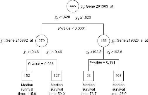
Classification tree for the lung cancer data generated by SSP with α = 0.2. The median survival time is in months.

Figure 3

Kaplan–Meier survival curves for the samples in the terminal nodes of the tree in Figure 2 for the lung cancer data.

As shown in Figure 4, the SDP approach at the type I error level of 0.05 gave two more splits to the tree generated by SSP. Regarding the splits at the children nodes of the root, the adjusted P-value for the split at the left child node is 0.009 (test statistic value 25.3, critical value 23.7) and the adjusted P-value for the split at the right child node is 0.013 (test statistic value 24.5, critical value 20.6). Among the terminal nodes in the third level of the tree in Figure 2, the second node from left is further split on Gene 207307_at at 7.35 (adjusted P-value, 0.005; test statistic value, 18.5; critical value, 16.8), and the fourth node from left is split on Gene 201509_at at 244.6 (adjusted P-value, 0.01; test statistic value, 18.3; critical value, 17.6). The median survival time of the left child node is more than double that of the right child node in each of these splits.

Figure 4

Classification tree for the lung cancer data generated by SDP with α = 0.2. The median survival time is in months.

For lung cancer data, the type I error level was chosen to be 0.2 in order to provide more information on classification using SSP. Because the P-value for the first split was ≫0.0001, we can find the classification tree with two terminal nodes when we use the significance level of 0.05 from Figure 2. This figure provides more information than using the 0.05 level. Because SDP adjusts the significance level at lower levels of the tree, we were able to get a large tree with the initial significance level of 0.05.

Discussion

We have proposed a method to control the type I error rate for tree classification by adopting the multiple testing concept. Our method allows us to avoid overfitting issues in tree classification when there are a large number of candidate predictors as in a prediction problem based on microarray data. Also proposed are two procedures, called SSP and SDP, to control the type I error rate using permutation method. Through simulations, we observe that both procedures control the type I error rate well. While SDP requires more computing time than SSP, the former tends to generate a larger tree than the latter when there exist prognostic predictors. To reduce the computing time, we may use SSP to construct a tree and then apply SDP to the terminal nodes derived from SDP.

Although SDP requires more computing time than SSP, SDP is preferred because it might provide more informative results and the computing power keeps improving. The type I error level was preassigned in this paper. To determine the type I error probability, we may search an optimal type I error probability in cross-validation at the training phase.

Matlab was used for the simulation and real data analysis. In the simulation, the computing time for generating a tree was approximately 20 seconds if there was no split. For trees with several splits, it took 45 seconds to 1 minute. For the gene imprinting data, it took approximately 9 hours to generate the tree by SSP on a Windows Vista 2.0 GHz machine. It will be much more efficient if SAS, R, or C is used. Using parallel computing might be practical for users.

We present an analysis of computing time under general settings. Assume n is the number of patients, m is the number of genes, and B is the number of permutations. Then, the running time of the log-rank statistic is O(n³m), and the running time of the critical value is O(n³mB). Here, we assume that the time spent for permutation for an array is constant. However, it is associated with n.

Once we find a splitting node, the n patients are split into two groups with sample sizes of n₁ and n₂ (n₁ + n₂ = n). We repeat the above process. Then, the running time of SSP is O(n³mB) + L·O(n³m) = O(n³mB). Here, L is the number of splits, which is negligible compared to B. The maximum possible value of L is log(n), which is the depth of a binary tree of n objects. The running time of SDP is L·O(n³mB) + L·O (n³m) = O(Ln³mB). Hence, the SDP approach is sensitive to the size of the tree.

Author Contributions

Conceived and designed the experiments: SHJ. Analyzed the data: YC, HA. Wrote the first draft of the manuscript: SHJ. Contributed to the writing of the manuscript: HA. Agree with manuscript results and conclusions: SHJ, HA, YC. Jointly developed the structure and arguments for the paper: SHJ, HA. Made critical revisions and approved final version: SHJ, HA. All authors reviewed and approved of the final manuscript.

References

Morgan

J.N.

, Sonquist

J.A.

Problems in the analysis of survey data, and a proposal. J Am Statl Assoc. 1963; 58: 415–34.

Breiman

, Friedman

J.H.

, Olshen

R.A.

, Stone

C.J.

Classification and Regression Trees. Belmont, California: Wadsworth; 1984.

Morgan

J.N.

, Messenger

R.C.

THAID: a Sequential Analysis Program for the Analysis of Nominal Scale Dependent Variables. Technical Report. Ann Arbor: Institute for Social Research, University of Michigan; 1973.

Quinlan

J.R.

C4.5: Programs for Machine Learning. San Mateo, California: Morgan Kaufmann; 1993.

Loh

W-Y

, Vanichsetakul

Tree-structured classification via generalized discriminant analysis (with discussion). J Am Stat Assoc. 1988; 83: 715–28.

Loh

W-Y

, Shih

Y.S.

Classification trees with unbiased multiway splits. Stat Sin. 1997; 7: 815–40.

Kim

, Loh

W-Y

. Split selection methods for classification trees. J Am Stat Assoc. 2001; 96: 589–604.

Kass

G.V.

An exploratory technique for investigating large quantities of categorical data. Appl Stat. 1980; 29: 119–27.

Hawkins

D.M.

FIRM: Formal inference-based recursive modeling, PC Version, Release 2.1. Technical Report 546, University of Minnesota, School of Statistics, 1997.

10.

Quanlan

J.R.

Simplifying decision trees. Int J Man-Mach Stud. 1987; 27: 221–48.

11.

Rissanen

Modeling by shortest data description. Automatica. 1978; 14: 465–71.

12.

Quinlan

J.R.

, Rivest

R.L.

Inferring decision trees using the minimum description length principle. Inf Comput. 1989; 80: 227–48.

13.

Mehta

, Rissane

, Agrawal

MDL-based decision tree pruning. In: Proceedings of the First International Conference on Knowledge Discovery and Data Mining (KDD'95) Montreal, Quebec, Canada. 1995; 216–21.

14.

Niblett

, Bratko

Learning Decision Rules in Noisy Domains, Research and Development in Expert Systems III. Cambridge: Cambridge University Press; 1986: 25–34.

15.

Bernau

, Augustin

, Boulesteix

A-L

. Correcting the optimal resampling-based error rate estimating the error rate of rate of wrapper algorithms. Biometrics. 2013; 69: 693–702.

16.

Tibshirani

, Tibshirani

Correction for the minimum error rate in cross-validation. Annals Appl Stat. 2009; 3: 822–9.

17.

Ding

, Tang

, Liao

S.G.

. Bias correction for selecting the minimal error classifier from many machine learning models. Bioinformatics. 2014: doi: 10.1093/bioinformatics/btu520.

18.

Greally

J.M.

Short interspersed transposable elements (SINEs) are excluded from imprinted regions in the human genome. Proc Nat Acad Sci. 2002; 99: 327–32.

19.

Shedden

, Taylor

J.M.G.

, Enkemann

S.A.

. Gene expression-based survival prediction in lung adenocarcinoma: a multi-site, blinded validation study. Nat Med. 2008; 14: 822–7.

20.

Reik

, Walter

Genomic imprinting: parental influence on the genome. Nat Rev Genet. 2001; 2(1): 21–32.

21.

, Dudoit

, Speed

T.P.

Resampling-based multiple testing for microarray data analysis. TEST. 2003; 12: 144.

22.

Dudoit

, Fridlyand

, Speed

T.P.

Comparison of discrimination methods for the classification of tumors using gene expression data. J Am Stat Assoc. 2002; 97: 77–87.

Type I Error Control for Tree Classification

Abstract

Keywords

Introduction

Methods

Single-step procedure

Step-down procedure

Permutation procedure for øl,α

Simulations

Real Examples

Gene imprinting data

Lung cancer data

Discussion

Author Contributions

References

Permutation procedure for ø_l,α