Sage Journals: Discover world-class research

Abstract

A new simulation model was created with a transfemoral prosthesis including a residual limb muscle model during the swing phase. The optimal knee joint friction value was calculated to minimize muscle metabolic energy expenditure. Using this model to examine how an amputee could walk as fast as possible, the minimum swing duration was calculated. The obtained optimal joint friction value was close to the value the subject preferred when walking normally. The calculated minimum swing duration was close to the time the subject could achieve. The method of dynamic optimization with a musculoskeletal model used in this study indicated the possibility of obtaining optimal mechanical properties suited to each amputee' capability of mastering control of his/her residual limb.

Keywords

Biomechanics of prosthetic/orthotic devices transfemoral prosthesis swing phase dynamic optimization musculoskeletal modeling

Introduction

Prosthetic knee joint mechanisms have a major influence on the swing phase control of the prosthetic gait of transfemoral amputees, which is one of the important factors in determining a gait pattern. Accordingly, determining the mechanical parameters of a prosthetic knee joint is an important problem, and several swing phase forward dynamic simulations have been performed to address it. 1–3 Compared to the inverse dynamics method for analyzing a prosthetic gait, 4,5 forward dynamic simulations have the advantages of being able to easily change parameters to test and evaluate prosthesis designs, and to analyze various gait conditions since the subject is not actually required to walk.

However, in previous simulation studies, the muscle properties of each residual limb were not included in the calculations; instead, a specific gait trajectory or the hip moment data of a particular amputee were used. Therefore, it was difficult to obtain the optimal prosthetic parameters suited to each amputee' physical capability, and to understand how the residual limb muscles control the prosthesis.

Meanwhile, musculoskeletal models, which consider muscle properties, have been used to perform forward dynamic simulations of a normal human gait, 6–8 but not of an amputee' gait. One reason is that a normal person' musculoskeletal data are not applicable to simulation of an amputee' gait because his or her muscle conditions have changed. In this

study, residual limb muscle properties were obtained from one subject using MR images and isometric force measurements.

There are two distinct and important types of gait problems, related to minimum and maximum effort. The first problem is that of obtaining prosthetic parameters that enable walking with minimum energy expenditure, i.e., those parameters enabling an amputee to walk most comfortably. In this study, knee joint friction was selected as the mechanical parameter to be optimized. This was because such friction markedly affects swing motion, 9 and an amputee can readily perceive the influence of any changes in joint friction. The second problem is to investigate whether a given prosthesis can effectively respond to an amputee' maximum effort, in other words, to examine to what extent an amputee can control the prosthesis in exerting his or her physical capabilities. One typical gait performance test is to have the amputee walk as fast as possible. With that in mind, we posed a minimum swing duration problem. The objectives of this study were to solve two problems, i.e., to obtain the optimal prosthetic mechanical parameters and to show how well the muscles could control the prosthesis, using a forward dynamic simulation with a musculoskeletal model of a residual limb.

Methods

Models

The model for the transfemoral prosthetic swing phase simulation consisted of an amputee' residual limb and a prosthesis. Because the swing motion is virtually limited to the sagittal plane, a two-dimensional planar model was constructed.

The patient modeled was a 19-year-old male, 173 cm in height and 55 kg in weight with a medium-length (18 cm) residual limb. This study was approved by the ethics review board of Rosai Rehabilitation Engineering Center, and informed consent was obtained from the patient. The iliopsoas, rectus-femoris, gluteus-maximus and hamstrings were selected for the musculoskeletal model of the residual limb since they are major muscles that contribute to hip-joint flexion and extension. 6,7 As atrophy of the amputated limb musculature is commonly observed, and as the muscle condition differs with each amputee, each muscle cross-section area and the origin and insertion points and pathways of those muscles were estimated using MR images of the subject. The MR images were analyzed using image-processing software (NIH image 1.62). The centroids of the attachment areas of muscles to bone were chosen as the origin and insertion points. The insertion points of the amputated muscles (rectus-femoris and hamstrings) were located at the distal end of the femur. The iliopsoas and the gluteus-maximus were considered to pass through via-points. The iliopsoas via-point was located in front of the iliopectineal eminence, and the gluteus-maximus via-point was located in back of the ischial tuberosity. The iliopsoas was divided into two muscles of psoas major and iliacus. The gluteus-maximus was divided into two muscles of the pass-through via-point muscle and straight line muscle. The force ratios of the divided muscles were assumed to be proportional to the ratio of muscle cross-section areas. The hip joint position was estimated to be at the center of the circle formed by the femoral head circumference on MR images. The moment arms were the perpendicular distance from the hip joint to the muscle pathways. Figure 1 shows the subject' residual limb muscle orientation. The model of each musculo-tendon unit was represented as a Hill-type muscle in series with an elastic tendon. 10 Using an isometric force-measuring device (Kawasaki Heavy Industries, Ltd, Japan), the relationship between the maximal isometric extension/flexion moment and the angle of the hip joint was obtained. In addition, the hip

Figure 1.

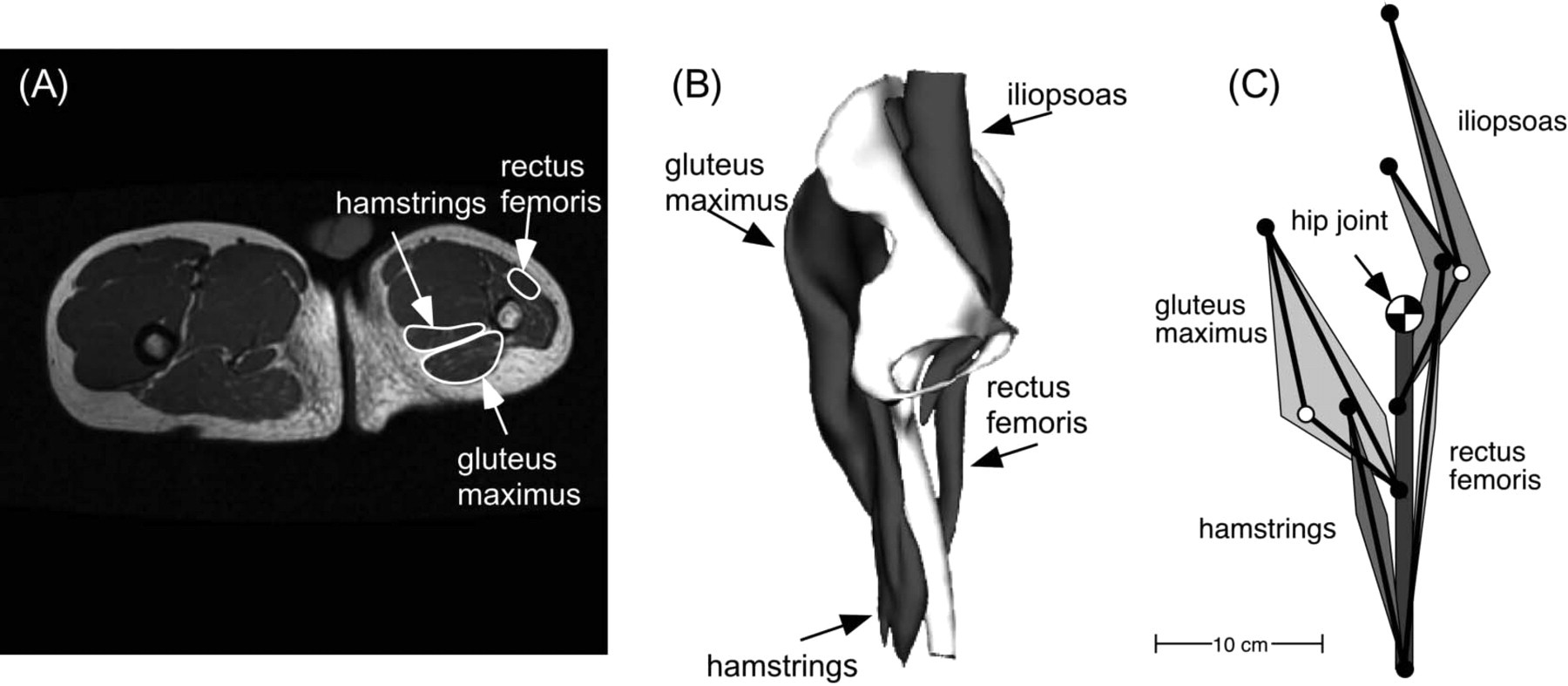
(A) MR image of subject' lower limb. Right side of the image shows residual limb. Slice is 10 cm below hip joint. (B) 3-D image of subject' residual limb. (C) Residual limb muscle diagram used in the model.

moment in the model was calculated using the muscle force exerted by a musculo-tendon unit and the moment arm. The musculo-tendon parameters (peak isometric force L^M _O, optimal muscle-fiber length L^M _O, and tendon slack length F^T _S) were obtained using a curve-fitting technique of the simplex method, 11 so that the calculated moments matched the measured moments. Here, F^M _O was assumed to be proportional to the muscle cross-section areas, non-amputated muscles (the iliopsoas and the gluteus-maximus) of L^M _O and L^T _S were assumed to be proportional to normal limb data, 22 and muscles were assumed to be fully activated.

The fabricated knee joint used and modeled in the present study was LAPOC-M730 (Imasen Engineering Corp., Japan) that had a single flexion-extension axis joint with adjustable friction, and was characterized by an extension-assist spring and a pneumatic cylinder to facilitate knee flexion and extension movements. Figure 2 shows a diagram of the knee joint mechanism. The displacement δ of spring and cylinder from the knee' full extension position is determined as a function of the knee flexion angle θ_k,

The spring force F_s is in proportion to δ,

where k is spring stiffness. The pneumatic cylinder force F_c is generated by cylinder pressures,

where P₁ is the pressure of the lower cylinder chamber, P₂ is the pressure of the upper cylinder chamber, and A is the piston area. The cylinder pressures are derived from

Figure 2

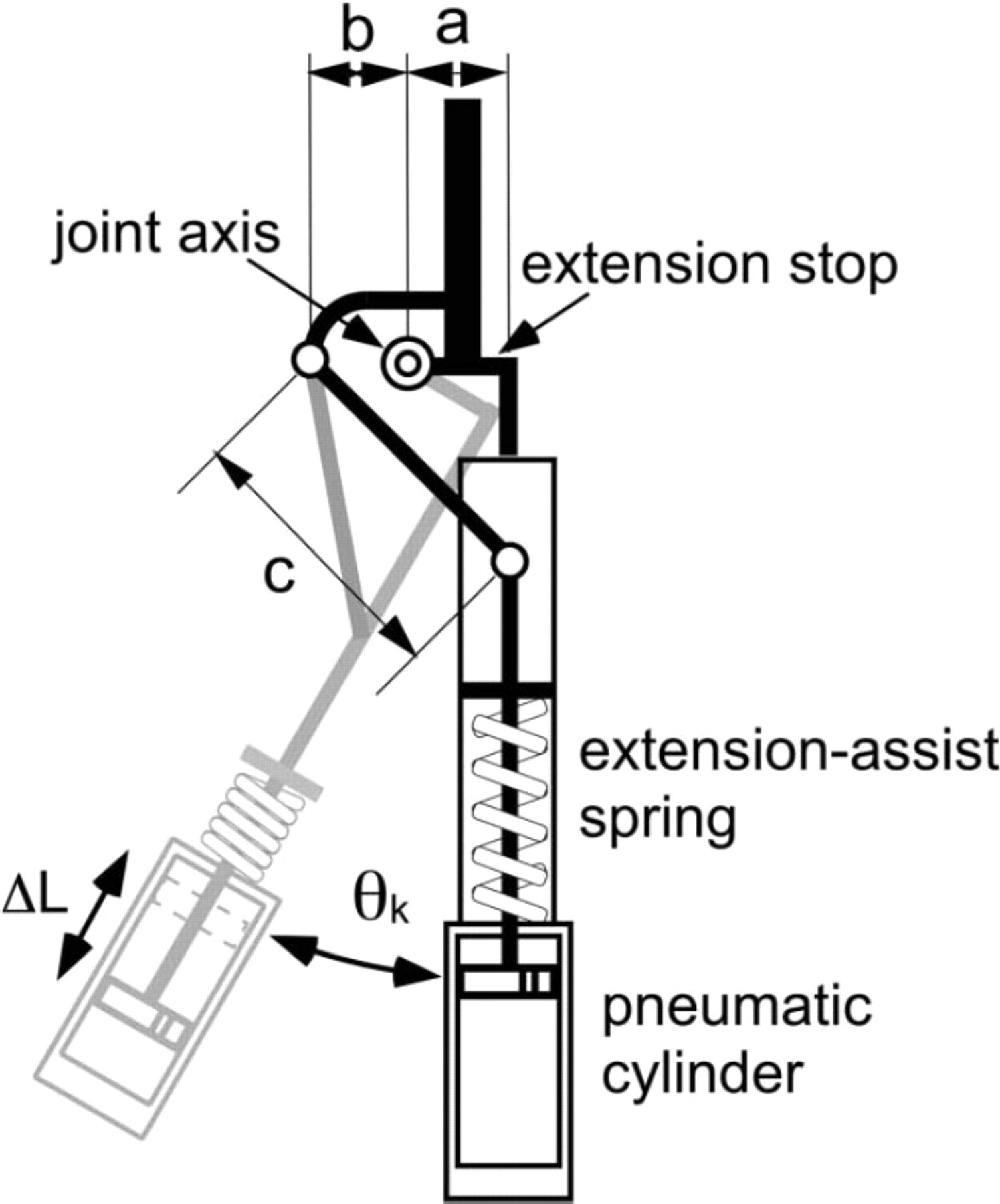
Knee joint mechanism. When knee flexion (angle θ_k) occurs in early swing phase, extension-assist spring is compressed and pneumatic cylinder piston is pushed downward to damp swing speed and prevent excess flexion. When knee extension occurs, extension-assist spring assists swing motion, pneumatic cylinder piston is pushed upward.

Navier-Stokes equations, and each cylinder pressure is the function of a differential equation including the cylinder volume and time-derivative of the cylinder volume. 12 Since the cylinder volume is changed by δ, the cylinder pressure P is expressed as

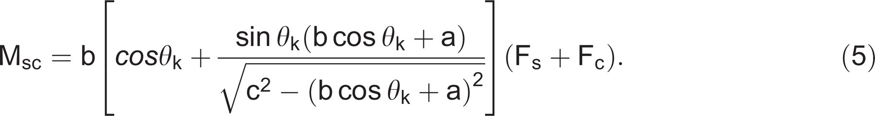
Through a link mechanism, the extension-assist spring force F_s and the pneumatic cylinder force F_c generate the knee moment M_sc,

The knee joint axis friction moment M_f is considered as constant, and its sign depends on the direction of flexion-extension. Accordingly, the knee joint moment M_k is expressed as,

The extension-assist spring stiffness, the pneumatic cylinder volume and the cylinder orifice diameter were obtained from engineering drawings of the knee joint.

As the socket of the prosthesis was considered to attach firmly to the residual limb, the prosthesis and the residual limb were modeled as one segment. Thus, the swing phase prosthesis model was assumed to be a double pendulum with a moving base. The equations of the double pendulum are formulated using Lagrange' Laws as

where I(θ) is the inertial matrix, and h(θ, θ) is the Coriolis, centripetal and gravitational moments, and hip acceleration, M=[M_h,M_k]^T is the vector of hip and knee moments and θ = [θ_t, θ_s]^T is the vector of thigh and shank angles in relation to the vertical. The hip joint moment M_h is generated by the residual limb musculoskeletal model. The mass and center of the mass of the prosthesis were measured directly, and the moment of inertia of the prosthesis was determined by the pendulum method. The mass and center of the mass and moment of inertia of the residual limb were calculated using human density and by stacking slices of the residual limb circumferences on MR images. The hip acceleration data were obtained from the subject' measured gait data.

Measurement of swing-phase kinematics

Swing-phase kinematics was measured using a motion-capture system with five cameras (VICON250, UK), and sagittal plane data were used. The subject was the same as the amputee modeled. Two reflective markers were attached to the lateral surface of the prosthetic ankle and knee joints. A hip joint marker was attached to the skin surface on the lateral side of the hip joint center. A force platform (Kistler, Switzerland, 40 × 200 cm) was used to determine the timing of heel contact and toe off of the prosthetic foot. The subject walked at his self-selected speed while kinematics and ground reaction forces were measured. The data were collected at a 200 Hz sampling frequency while the kinematics data were low-pass filtered using a Butterworth filter with a cut-off frequency of 8 Hz. For those measurements, the knee joint axis friction was changed randomly at five different values. Under each condition, five gait trials were performed. After each trial, the walking subject informed us of his comfort level, and at the end of the trial, he selected the most preferable knee joint friction value for comfortable walking.

For evaluation of the minimum swing duration, the subject was asked to walk at maximum speed while the swing duration was measured. When trying to maximize walking speed, the subject felt discomfort upon terminal impact, i.e., the impact experienced when the knee extension was mechanically forced to stop at full extension. Then the subject began to control the knee joint angular velocity to reduce the impact.

Simulations and dynamic optimization problem

An optimal control method was applied to solve the dynamic optimization problem of the transfemoral prosthesis during the swing phase. The optimal control involved a process of determining the control variables of a dynamic system to minimize an objective function. The dynamic system is described by the following differential equation:

In this system, the state variables x were muscle activations a_m(t) 10 (m being the muscle numbers 1 to 4) in the musculoskeletal model, the knee joint pneumatic cylinder pressures P₁ and P₂ (Equation 4), the lower limb angles (θ_t, θ_s), and the angular velocities ( $\dot{θ}$ _t, $\dot{θ}$ _s). Those angles and angular velocities were derived from double-pendulum equations (Equation 7), which included both the musculoskeletal and knee joint mechanism models. The control variables, u, were muscle excitation signals u_m(t) (0 <u_m(t) < 1) that determine the value of muscle activations a_m(t). For greater calculation efficiency, each muscle excitation signal was divided into twenty periods, u_mi(t) (i = 1 to 20) within the swing phase.

More than 20 periods in the muscle excitation signal requires much calculation time, and a small number of periods produces inaccurate results. 13 To obtain an optimal knee joint friction value, friction was also added to the control variables. A selected objective function, J, in this study was intended to minimize the expenditure of metabolic energy, which had been used as a gait performance criterion. That expenditure was obtained based on the literature 14 using a musculoskeletal model.

The swing phase system includes boundary conditions of the angle and angular velocity of thigh and shank. Using the terminal values of thigh angle θ_tT, shank angle θ_ST, thigh angular velocity $\dot{θ}$ _tT and shank angular velocity $\dot{θ}$ _ST, the terminal conditions at the moment of heel contact t_f can be expressed as terminal equality constraints as follows:

These constraints were added to the object function as a condition to minimize

where the weight factors w were started from 0.001 and gradually increased by the penalty-multiplier method. 15 Additionally, for terminal impact, a constraint condition according to which the knee joint angular velocity must be less than c was added to the calculation. The constant c was the maximum knee extension angular velocity obtained from measured data. If the knee joint angular velocity $\dot{θ}$ _k was greater than c, the object function was modified including the constraint condition to

The values in initial conditions, terminal conditions, joint angular velocity constraints and swing duration were obtained from the subject' average measurements. As a result of these calculations, lower limb joint angle trajectories, muscle excitation signals and knee joint friction were obtained.

Custom-made software written in Fortran 77 was used to solve these problems, while a quasi-Newton method (IMSL Library) 16 was used to solve optimization problems. To avoid convergence to a local minimum, the calculations were performed with different initial control variables.

With a minimum swing duration problem, the objective function J was the swing duration. t_f Instead of joint friction, swing duration was selected as one of the control variables to determine, and the joint friction was set at a constant 1.2 Nm. For calculation convenience, dynamic equations were parameterized by normalized time τ = t/t_f 13 as

Table I.

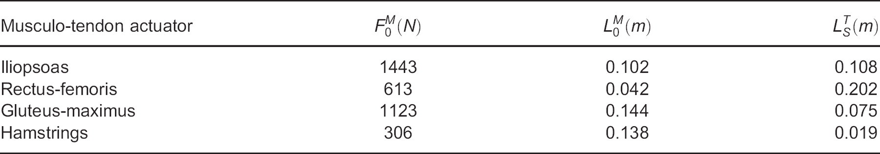
Residual limb musculo-tendon parameters of peak isometric force F^M ₀ optimal muscle-fiber length L^M ₀, and tendon slack length L^T _S

Musculo-tendon actuator	F^M ₀(N)	L^M ₀(m)	L^T _S(m)
lliopsoas	1443	0.102	0.108
Rectus-femoris	613	0.042	0.202
Gluteus-maximus	1123	0.144	0.075
Hamstrings	306	0.138	0.019

Results

The muscle parameters obtained (peak isometric force, F^M ₀, optimal muscle-fiber length, L^M ₀, and tendon slack length, L^T _S) are shown in Table I.

The knee joint friction obtained by the optimal calculation needed to minimize muscle metabolic energy expenditure was 1.8 Nm, and the result of sensitivity analysis showed that the friction differences of 1% from the minimum energy expenditure ranged from 1.0–2.7 Nm (Figure 3). On the other hand, the subject could walk at various knee joint friction values (0.3, 0.7, 1.2, 2.1 and 3.5 Nm), among which he preferred 1.2 Nm for maximum walking comfort. However, he indicated that the differences among 0.7, 1.2 and 2.1 Nm were so small that distinguishing one from another was difficult. He also found it difficult to control gait timing with 0.3 Nm friction, and tended to tire easily with 3.5 Nm friction. A comparison of calculated and measured data for the lower limb motion trajectory and residual limb muscle forces is shown in Figure 4. The calculated trajectory of the lower limb approximated our experimental results. The flexor forces were generated in the early swing phase and the extensor forces in the late swing phase. These muscle output timings were basically similar to those reported in the transfemoral residual limb EMG data. 17,18

The measured swing duration of this subject during normal walking was 0.48 sec. However, he was able to reduce his swing duration to 0.43 sec, and the calculated result of his minimum swing duration was 0.41 sec. The calculated results of hip muscle forces are shown in Figure 5. Compared to Figure 4B, the muscle forces of both flexors and extensors were greater than the normal gait (the iliopsoas was about 1.5 times greater at the initial swing phase, while the gluteus-maximus was 2.1 times greater at the late swing phase). The hip flexor force was temporarily generated just before full knee extension. This timing corresponded to that of the angular velocity constraint to reduce terminal impact.

Figure 3.

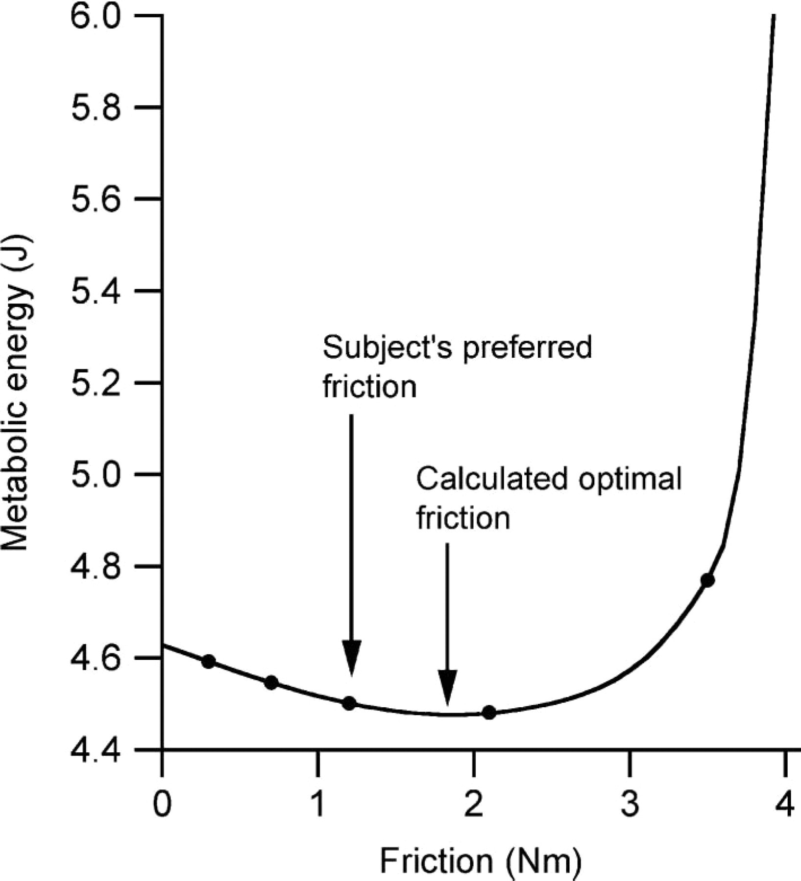
Results of sensitivity analysis of knee joint axis friction for metabolic energy expenditure. Measured friction was 0.3, 0.7, 1.2, 2.1 and 3.5 Nm (dot symbols). Subject' preferred friction was 1.2 Nm, and calculated optimal friction was 1.8 Nm.

Figure 4

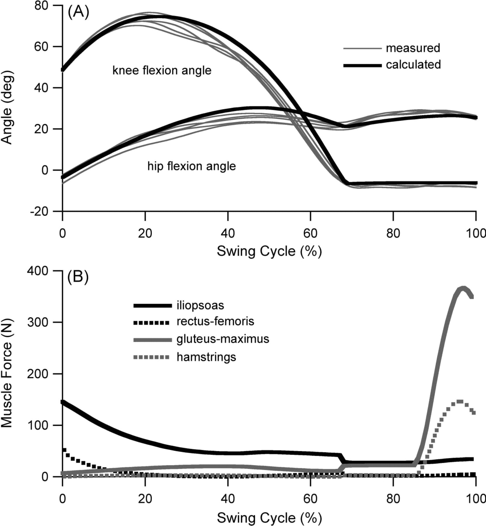
(A) Results of measured (thin grey lines, with subject preferred knee joint friction 1.2 Nm, five repeated trials under the same gait conditions) and calculated (thick black lines, with the same joint friction as measured) lower limb angle during swing phase of normal gait. The hip flexion angle is the thigh angle in relation to the vertical, and the knee flexion angle is the shank angle in relation to the thigh. (B) Result of calculated residual limb muscle forces.

Discussion

The results of sensitivity analysis (Figure 3) indicated that a wide range of knee joint friction was required to minimize energy expenditure, while the change in energy expenditure within this range was small. This may explain why the subject could not clearly distinguish between 0.7, 1.2 and 2.1 Nm. On the other hand, at a friction greater than 3.5 Nm), the sensitivity analysis showed a steep increase in energy expenditure. At the calculated maximum friction of 4.1 Nm, the energy expenditure was 60% greater than the minimum expenditure and might cause considerable fatigue. Therefore, from the standpoint of energy expenditure, though an optimal friction value existed, the allowable friction range was wide.

With regard to minimum swing duration, the calculation results revealed an extensive shortening of the swing duration that was close to that possible for the subject. Although the muscle forces were greater than with a normal gait, maximum forces during the swing phase

Figure 5

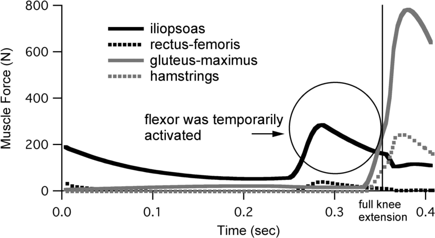
Results of calculated residual limb muscle forces on minimum swing duration calculations. Flexors (iliopsoas and rectus-femoris) were temporarily activated just before full extension occurred at 0.35 sec.

appeared to be smaller than expected. This was because the flexor force had to be restrained in the initial swing phase, while not increasing the swing speed too much in order to reduce the terminal impact. Also, the flexor force had to be generated just before full knee extension to reduce that impact. Once the terminal impact was reduced by a prosthetic mechanism, the subject could walk with a shorter swing duration.

As shown in Figure 4A, the result of simulation of lower limb angles resembled the results of measurements. This showed the validity of our method to emulate the swing phase kinematics of a transfemoral prosthesis. As for kinetic properties, the predicted muscle force patterns in Figure 5 were qualitatively consistent with the EMG data of the transfemoral amputee.

The present study examined one subject with a medium-length residual limb considered to be representative of typical amputees. The ability to control a prosthesis depends on the length of the residual limb. Construction of musculoskeletal models for various lengths of residual limbs using both tomographic images and measured force data of residual limb muscles would enable a variety of amputee gait simulations.

The musculoskeletal model parameters (Table I) that may affect our results should be discussed. The peak isometric muscle force (F^M ₀ is considered to depend on the physiological cross-sectional area (PCSA). The average of the peak isometric muscle force per PCSA in our model was 56 N/cm², higher than the 38 N/cm 2 and 35 N/cm 2 cited in earlier reports. 19,20 Calculation of maximal isometric hip moments using these reported data produced values smaller than our measured values. One reason for this discrepancy might be the limited number of modeled muscles. In fact, there are more muscles involved in hip extension/flexion. For model precision, inclusion of all muscles related to the hip joint would be desirable. However, using more than five muscles can lead to inconsistent results because of the many unknown parameters. When the maximal isometric hip moments were calculated using a musculoskeletal model of a normal limb including all related muscles, 21 the four major muscles alone produced 78% of total moment in extension and 60% in flexion. If our model included all related muscles, peak isometric muscle force per PCSA would become around (56N/cm 2 x 0.78 + 56N/cm 2 x 0.6)/2 = 39N/cm², a value that is close to reported values. Thus, with the four major muscles representing all related hip muscles, the force of each muscle force looked larger than expected. The length-related parameters (optimal muscle-fiber length, L^M ₀ and tendon slack length, L^T _S) of the iliopsoas and the gluteus-maximus were similar to the reported data for healthy humans. 21,22 On the

other hand, the length-related parameters of the rectus-femoris and hamstrings were shorter than the reported data because of amputation.

The models of this study were two-dimensional models. To analyze hip joint motion with adduction/abduction or rotation like circumduction gait, three-dimensional models should be constructed. As normal gait is confined within the sagittal plane, a two-dimensional model is acceptable for analysis of normal swing phase kinematics.

Conclusions

Numerical simulations of the prosthetic swing phase were performed using a musculoske-letal model of the residual limb. Our simulations not only provided the optimal mechanical parameters of a prosthesis, but also showed approximately how the muscles in the residual limb controlled the prosthesis. The simulation results were approximately consistent with the measured data and gave the expected parameter values for the subject. Our results indicate the possibility that the optimal prosthetic mechanical properties for any amputee could be obtained by constructing an individual musculoskeletal model.

Acknowledgements

The author would like to acknowledge Mr T. Yamashita, C.P.O., for technical assistance, and Dr T. Aoyama and Dr E. Genda for clinical comments.

Declaration of interest : The author reports no conflicts of interest. The author alone is responsible for the content and writing of the paper.

References

Tsai

Mansour

. Swing phase simulation and design of above knee prostheses. J Biomech Eng 1986; 108(1): 65–72.

Wang

Tsuei

. Adaptative control of above knee electro-hydraulic prosthesis. J Biomech Eng 1992; 114(3): 421–424.

Beck

Czerniecki

. A method for optimization of above-knee prosthetic shank-foot inertial characteristics. Gait Posture 1994; 2: 75–84.

Yang

Solomonidis

Spence

Paul

. The influence of limb alignment on the gait of above-knee amputees. J Biomech 1991; 24(11): 981–997.

Boonstra

Schrama

Fidler

Eisma

. Energy cost during ambulation in transfemoral amputees: A knee joint with a mechanical swing phase control vs. a knee joint with a pneumatic swing phase control. Scand J Rehabil Med 1995; 27(2): 77–81.

Davy

Audu

. A dynamic optimization technique for predicting muscle forces in the swing phase of gait. J Biomech 1987; 20(2): 187–201.

Yamaguchi

Zajac

. Restoring unassisted natural gait to paraplegics via functional neuromuscular stimulation: A computer simulation study. IEEE Trans Biomed Eng 1990; 37(9): 886–902.

Neptune

Kautz

Zajac

. Contributions of the individual ankle plantar flexors to support, forward progression and swing initiation during walking. J Biomech 2001; 34(11): 1387–1398.

Wilson

Jr.

Transfemoral prosthetic components: Variations, indications, contraindications. In: Bowker

Michael

, editors. Atlas of limb prosthetics: Surgical, prosthetic and rehabilitation principles. St Louis, MO: Mosby; 1992. pp 523–533.

10.

Zajac

. Muscle and tendon: Properties, models, scaling, and application to biomechanics and motor control. Crit Rev Biomed Eng 1989; 17(4): 359–411.

11.

Hatze

. Estimation of myodynamic parameter values from observations on isometrically contracting muscle groups. Eur J Appl Physiol Occup Physiol 1981; 46(4): 325–338.

12.

Zarrugh

Radcliffe

. Simulation of swing phase dynamics in above-knee prostheses. J Biomech 1976; 9(5): 283–292.

13.

Pandy

Anderson

Hull

. A parameter optimization approach for the optimal control of large-scale musculoskeletal systems. J Biomech Eng 1992; 114(4): 450–460.

14.

Bhargava

Pandy

Anderson

. A phenomenological model for estimating metabolic energy consumption in muscle contraction. J Biomech 2004; 37(1): 81–88.

15.

Navon

Villiers

. Combined penalty multiplier optimization methods to enforce integral invariants conservation. Monthly Weather Rev 1983; 111: 1228–1243.

16.

IMSL. Math/Library Bcong/Dbcong. Fortran Subrout Math Applic 1991; 1036–1042.

17.

Jaegers

Arendzen

de Jongh

. An electromyographic study of the hip muscles of transfemoral amputees in walking. Clin Orthop 1996; (328): 119–128.

18.

Hong

Mun

. Relationship between socket pressure and EMG of two muscles in trans-femoral stumps during gait. Prosthet Orthot Int 2005; 29(1): 59–72.

19.

Haxton

. Absolute muscle force in the ankle flexors of man. J Physiol 1944; 103: 267–273.

20.

Cholewicki

McGill

Norman

. Comparison of muscle forces and joint load from an optimization and EMG assisted lumbar spine model: Towards development of a hybrid approach. J Biomech 1995; 28(3): 321–331.

21.

Delp

Loan

Hoy

Zajac

Topp

Rosen

. An interactive graphics-based model of the lower extremity to study orthopaedic surgical procedures. IEEE Trans Biomed Eng 1990; 37(8): 757–767.

22.

Friederich

Brand

. Muscle fiber architecture in the human lower limb. J Biomech 1990; 23(1): 91–95.

Dynamic Optimization of Transfemoral Prosthesis during Swing Phase with Residual Limb Model

Abstract

Keywords

Introduction

Methods

Models

Measurement of swing-phase kinematics

Simulations and dynamic optimization problem

Results

Discussion

Conclusions

Acknowledgements

References