Sage Journals: Discover world-class research

Abstract

Earthquake site responses or site effects are the modifications of surface geology to seismic waves. How well can we predict the site effects (average over many earthquakes) at individual sites so far? To address this question, we tested and compared the effectiveness of different estimation techniques in predicting the outcrop Fourier site responses separated using the general inversion technique (GIT) from recordings. Techniques being evaluated are (a) the empirical correction to the horizontal-to-vertical spectral ratio of earthquakes (c-HVSR), (b) one-dimensional ground response analysis (GRA), and (c) the square-root-impedance (SRI) method (also called the quarter-wavelength approach). Our results show that c-HVSR can capture significantly more site-specific features in site responses than both GRA and SRI in the aggregate, especially at relatively high frequencies. c-HVSR achieves a “good match” in spectral shape at ∼80%–90% of 145 testing sites, whereas GRA and SRI fail at most sites. GRA and SRI results have a high level of parametric and/or modeling errors which can be constrained, to some extent, by collecting on-site recordings.

Keywords

Site response site effects HVSR ground response analysis square-root-impedance earthquake

Introduction

Surface geology can modify incoming seismic waves, and these modifications are denoted as “site effects” or “site responses.” Site effects arise due to the presence of impedance (the product of wave velocity and density) contrasts, surface and subsurface topographies, and so on. Currently, various approaches are available to quantify site effects in seismic hazard and risk assessments.

One approach to capture site effects is to utilize generic prediction models relating amplifications to various predictor variables (Table 1). Predictor variables can be (a) site parameters from in-situ geotechnical/geophysical measurements, for example, average shear-wave velocity in the topmost 30 m (V_S₃₀), sediments thickness, and site resonant frequency (e.g. Hassani and Atkinson, 2018; Kwak and Seyhan, 2020); or (b) proxies from existing regional models or maps, for example, topographic slope, terrain, and geology (e.g. Wald and Allen, 2007; Weatherill et al., 2020; Yong et al., 2012). Models in the first group are often embedded in recent ground-motion models (GMMs; e.g. Boore et al., 2014), whereas those in the second category are applied in regional or global site-response mapping. One needs to balance the spatial coverage and precision when considering these models.

Table 1.

Various techniques to quantify earthquake site responses

Approach	Description	Prerequisite	Reference	Note
SSR	Standard spectral ratio	Simultaneous recordings at the target and its nearby outcrop rock site (free of site effects)	Outcrop rock	Observation
SBSR	Surface-to-borehole spectral ratio	Simultaneous recordings at collocated surface-downhole pair	Rock at depth	Observation
δS2S	Site term from analyses to GMM residuals	Multiple stations with recordings from multiple events to which the selected GMM is applicable	Single site or a set of sites	Observation
GIT	General inversion technique	Multiple stations with recordings from multiple events	Single site or a set of sites	Observation
GRA	Ground response analysis	1D site model (density, velocity and damping profiles, modulus reduction, and damping curves)	Outcrop rock or rock at depth	Numerical modeling
SRI	Square-root-impedance	1D site model (density and velocity profiles, attenuation parameter)	Outcrop rock	Analytical approx.
c-HVSR	Corrected horizontal-to-vertical spectral ratio	Vertical correction functions (and site parameters) and HVSR function	Outcrop rock or rock at depth	Empirical prediction
Amp	Generic site-response models	Site parameter(s)	Outcrop rock	Empirical prediction

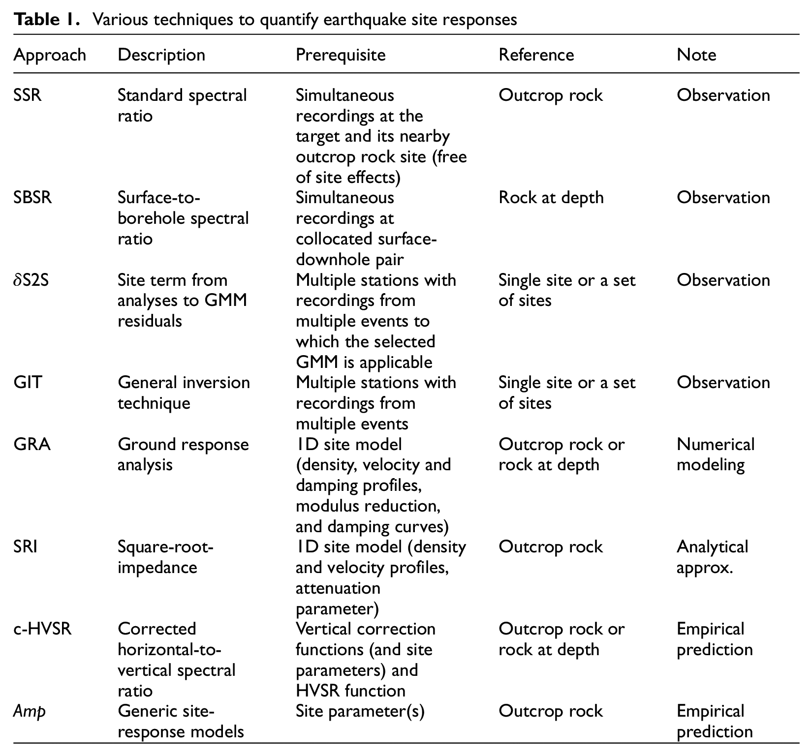
In addition, site responses at specific sites can be estimated using one-dimensional (1D) ground response analysis (GRA) or the square-root-impedance (SRI) method (Table 1). GRA assesses site responses by modeling the propagation of vertically incident plane SH waves through horizontally stratified sedimentary layers (i.e. the “1DSH” assumptions). In contrast, SRI is based on the ray theory and only uses quarter-wavelength (QWL) velocities and densities corresponding to the frequency of interest (Boore, 2003; Joyner et al., 1981). Both approaches require a detailed site model, and GRA also needs soil nonlinear properties for equivalent linear or nonlinear analyses.

Another site-specific technique is the empirical correction to the ratio of the Fourier spectrum of the horizontal component to that of the vertical component, namely the horizontal-to-vertical spectral ratio (HVSR, Nakamura, 2019) (Table 1). We denote this correction to HVSR as the “c-HVSR” method. Based on the diffuse field theory, Kawase’ team (Ito et al., 2020; Kawase et al., 2018b) proposed this technique, and Zhu et al. (2020c) considered it as an empirical approach and evaluated its performance in comparison with GRA using surface-downhole recording pairs. c-HVSR does not require any site models but needs on-site recordings and pre-defined correction functions for the study region.

How well can we predict site effects so far using these estimation techniques (GRA, SRI, c-HVSR, and generic site-response models)? Addressing this question is crucial to identify the current best approach and then adopt and iterate on the best practice. However, there are a few hurdles in comparing various techniques. First, we need reliable site-response observations that could be utilized as “benchmark,”“gold standard,” or “ground-truth” data to evaluate or calibrate other estimation approaches/models. In addition, we need detailed site metadata (e.g. 1D site models and seismic recordings) to test all these approaches at common sites.

However, such a comprehensive and robust evaluation can be realized, thanks to the large volume of ground-motion data accumulated on the dense strong-motion networks, K-NET, and KiK-net, in Japan, with detailed site information (National Research Institute for Earth Science and Disaster Resilience, 2019). Thus, a reliable site-response dataset is established from the recordings for a large number of sites through the general inversion technique (GIT) (Nakano et al., 2015), empirical ground-motion modeling (site term δS2S_s, Loviknes et al., 2021), and surface-to-borehole spectral ratio (SBSR, Zhu et al., 2020b) (Table 1). These site-response data are unique in that they were derived in the Fourier domain, as to our knowledge, the first such dataset. This makes it possible to study the site-response variability at high frequencies, for example, f > 10 Hz. Furthermore, an open-source site database is also recently made available for these stations (Zhu et al., 2021b). Given these latest developments, the effectiveness of current site-response estimation techniques can be tested and compared on the same dataset under one framework. In this article, we focus on the evaluation of GRA, SRI, and c-HVSR. Results on site-response models by classic regressions and machine learning are presented in a separate article.

We first develop a framework to evaluate the effectiveness of different site-response estimation techniques. Then we present the benchmark site-response data, that is, Fourier site responses derived using GIT with reference to outcrop rock conditions (V_S = 3.45 km/s), and the site metadata, at 1725 K-NET and KiK-net sites. Next, we introduce the three approaches, including GRA, SRI, and c-HVSR, before the testing and comparison of their performance in predicting observed site responses. Furthermore, we discuss two strategies to potentially improve the efficacy of GRA and SRI, including using HVSR-consistent V_S profiles and site-specific attenuation measurements.

Evaluation framework

Site-to-site variability $ϕ_{S 2 S}^{m}$

If multiple recordings are available at multiple sites, observed site response at a site s during earthquake e can be expressed as:

A F_{e s} = a + δ S 2 S_{s}^{0} + δ W_{e s},

(1)

δ S 2 S_{s}^{0} ~ N (0, ϕ_{S 2 S}^{0}),

(2)

δ W_{es} ~ N (0, ϕ_{SS}),

(3)

where $A F_{es}$ is the observed site response at a specific site s during an earthquake e, a is a constant and denotes the mean AF_es across all sites in the dataset, $δ S 2 S_{s}^{0}$ is the mean site response at the site s over all events relative to the global mean a, and $δ W_{es}$ represents the deviation of site response of a given earthquake from the site-specific mean response $δ S 2 S_{s}^{0}$ . In ground-motion modeling, $δ S 2 S_{s}^{0}$ and $δ W_{es}$ are often treated as independent and normally distributed random variables with zero means and standard deviations $ϕ_{S 2 S}^{0}$ and $ϕ_{SS}$ , respectively. $ϕ_{S 2 S}^{0}$ and $ϕ_{SS}$ denote the site-to-site (intersite) and within-site (intrasite) variabilities in site response, respectively. All the terms in the above equations are frequency-dependent; however, f is omitted for simplicity.

In this study, we only focus on the repeatable site response at a given site, that is, $a + δ S 2 S_{s}^{0}$ , and the event-specific residual and the randomness in site response are investigated by Zhu et al. (2021a). Currently, the repeatable site response at a target site can be estimated through various methods (m). The estimation can be through the use of a site characterization proxy, for example, V_S₃₀, site resonant frequency f₀, sediment thickness Z_x (x = 0.8, 1.0, 1.5, and 2.5 km/s), topographic indices, or their combinations, and GRA, SRI, and c-HVSR. When multiple sites are investigated, the residual between observation ( $a + δ S 2 S_{s}^{0}$ ) and prediction ( $μ_{s}^{m}$ ) using method m can be partitioned into a constant term $c^{m}$ and a site-specific term $δ S 2 S_{s}^{m}$ :

Resi d_{s} = (a + δ S 2 S_{s}^{0}) - μ_{s}^{m} = c^{m} + δ S 2 S_{s}^{m},

(4)

δ S 2 S_{s}^{m} ~ N (0, ϕ_{S 2 S}^{m}),

(5)

where $a + δ S 2 S_{s}^{0}$ is the repeatable site response at site s, $μ_{s}^{m}$ is the site-specific prediction of site response using method m, $c^{m}$ represents the overall bias of the method m in site effect estimation at selected sites, and $δ S 2 S_{s}^{m}$ is the remaining site effects at site s and represents the portion not captured by the estimation technique m. $δ S 2 S_{s}^{m}$ is also considered as a normally distributed variable with zero mean and standard deviation $ϕ_{S 2 S}^{m}$ . $ϕ_{S 2 S}^{m}$ represents the site-to-site (intersite) variability in the residual site response uncaptured by m across all sites in a dataset, and it includes all sources of uncertainties, both parametric and modeling uncertainties, in applying the approach m to assess site effects.

Though $ϕ_{S 2 S}^{m}$ is often treated as aleatory variability within the GMM framework, it is epistemic. In an ideal case, site-specific amplification could be fully captured, and thus $ϕ_{S 2 S}^{m}$ can be reduced to zero. However, conventional site-response estimation techniques can only partially capture $a + δ S 2 S_{s}^{0}$ , thus $ϕ_{S 2 S}^{m}$ is well above zero (lower bound) but lower than $ϕ_{S 2 S}^{0}$ (upper bound) to different extents. The degree of reduction of $ϕ_{S 2 S}^{m}$ relative to $ϕ_{S 2 S}^{0}$ reveals to what extent the approach m can capture the site-specificness of amplification at these sample sites.

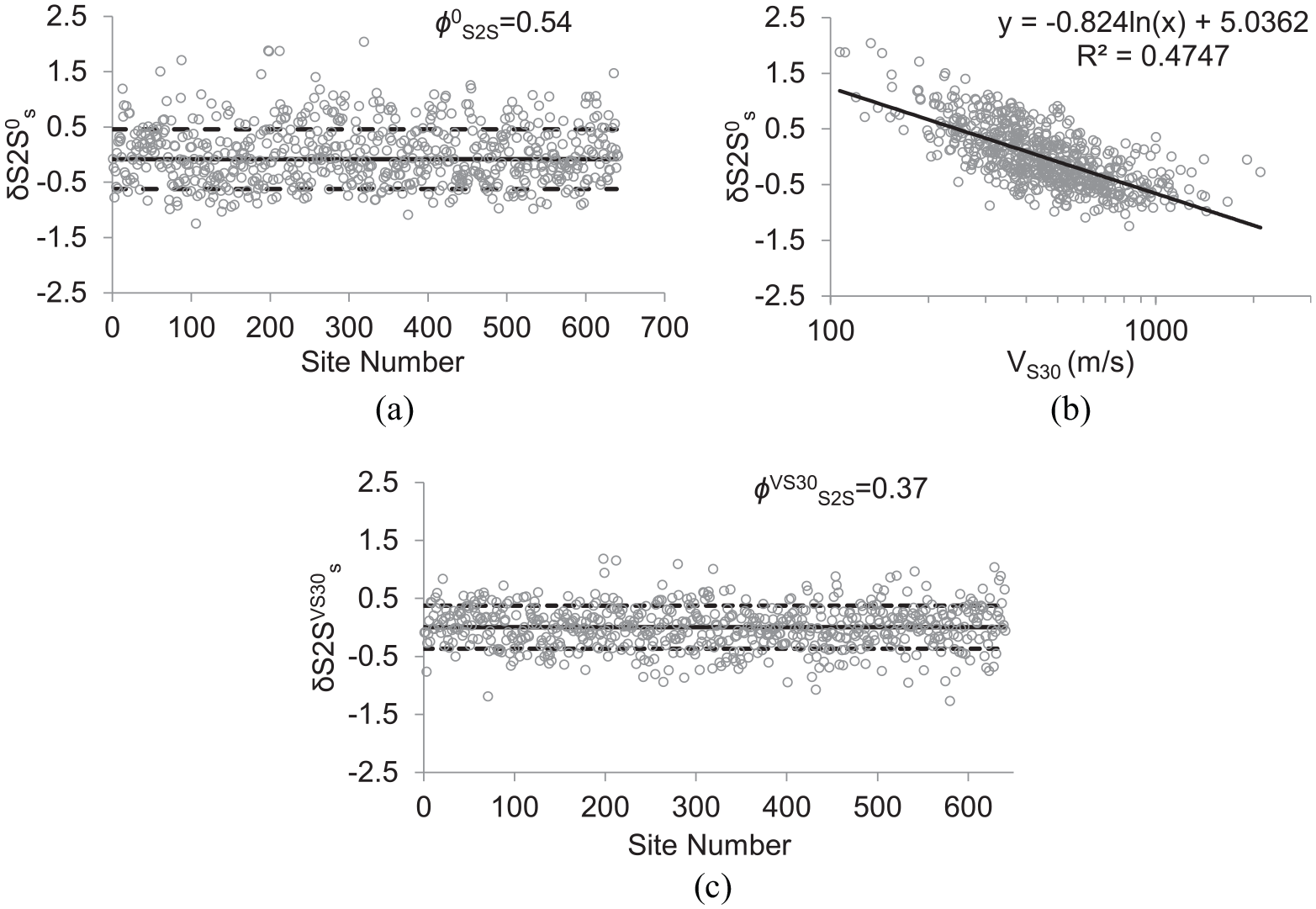
Figure 1 further illustrates this issue. Figure 1a depicts the site responses $δ S 2 S_{s}^{0} s$ (after removing their mean a) at f = 1.0 Hz for 641 KiK-net stations. The standard deviation of $δ S 2 S_{s}^{0}$ is $ϕ_{S 2 S}^{0}$ = 0.54 for this dataset. $δ S 2 S_{s}^{0}$ is linearly correlated with V_S₃₀, as shown in Figure 1b. Thus, for illustration purposes, we simply model $δ S 2 S_{s}^{0}$ as a linear function of V_S₃₀. Residual site responses, that is $δ S 2 S_{s}^{VS 30}$ , are plotted in Figure 1c with standard deviation ϕ^VS30_S2S = 0.37. ϕ^VS30_S2S is much lower than $ϕ_{S 2 S}^{0}$ by 0.17 (ln scales). The amount of reduction quantifies the effectiveness of V_S₃₀ in modeling site response at f = 1.0 Hz.

Figure 1.

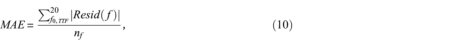
(a) Observed site responses $δ S 2 S_{s}^{0}$ (ln scales) at f = 1.0 Hz at KiK-net sites, and ϕ⁰_S2S is the standard deviation of $δ S 2 S_{s}^{0}$ . Solid and dashed lines correspond to the mean and mean ± one standard deviation values, respectively. (b) $δ S 2 S_{s}^{0}$ is modeled as a linear function of V_S₃₀ (ln scales), and the solid line represents the linear fit. (c) Residual site response $δ S 2 S_{s}^{VS 30}$ after removing the portion associated with V_S₃₀, and ϕ^VS30_S2S is the standard deviation of $δ S 2 S_{s}^{VS 30}$ and is lower than ϕ⁰_S2S.

Goodness-of-fit metrics

$ϕ_{S 2 S}^{m}$ represents the overall performance of a given approach over sample sites, but it does not reflect its efficacy at any individual site. Thus, to evaluate the degree of match between observation and prediction at a specific site, we also use goodness-of-fit (GoF) measures: Pearson’s r (Equation 6), Spearman’s ρ (Spearman, 1907, Equation 7), and Kendal’s τ. Pearson’s r measures the strength of linear correlation between two variables and is adopted by many preceding studies (e.g. Thompson et al., 2012). However, Pearson’s r requires normality and no extreme outliers of two variables, thus we also utilize two nonparametric metrics without such prerequisites, that is, Spearman’s ρ and Kendal’s τ which assess the ordinal relationship between two variables. All three GoF metrics measure the closeness in spectral shape (alignment of peaks and troughs) and have values ranging from −1 (a total negative correlation) to 1 (a total positive correlation). Since theoretical transfer functions (TTFs) from GRA and SRI are not so meaningful to use for frequencies below f_{0, TTF} (fundamental resonant frequency on TTF at a given site), these GoF metrics are derived in the frequency range from f_{0, TTF} to 20 Hz.

r = \frac{\sum_{i = 1}^{n} (x_{i -} \bar{x}) (y_{i -} \bar{y})}{\sqrt{\sum_{i = 1}^{n} {(x_{i -} \bar{x})}^{2}} \sqrt{\sum_{i = 1}^{n} {(y_{i -} \bar{y})}^{2}}},

(6)

ρ = \frac{cov (r g_{x}, r g_{y})}{σ_{r g_{x}} σ_{r g_{y}}},

(7)

τ = \frac{2 \sum_{i = 1}^{n - 1} \sum_{j = i + 1}^{n} [sgn (x_{i -} x_{j}) sgn (y_{i -} y_{j})]}{n (n - 1)},

(8)

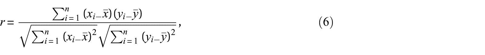
where n is the sample size (the number of stations in this research); x and y are the vectors of observation and prediction, respectively; x_i and y_i denote the ith (i = 1, 2, ..., n) elements of x and y; $\bar{x}$ and $\bar{y}$ denote means of x and y; rg_x and rg_y denote the vectors of rank values of elements in x and y; $σ_{r g_{x}}$ and $σ_{r g_{y}}$ denote the standard deviations of rg_x and rg_y; cov denotes covariance operation; and sgn denotes the sign function. In addition to the three relative GoF measures, the degree of match in amplitude between observed and predicted site responses is gauged in the absolute term using mean absolute error (MAE):

Resid (f) = lnAm p_{obs} (f) - lnAm p_{pred} (f),

(9)

MAE = \frac{\sum_{f_{0, TTF}}^{20} | Resid (f) |}{n_{f}},

(10)

where $Am p_{obs} (f)$ and $Am p_{pred} (f)$ represent the observed and predicted amplification functions, respectively. n_f is the number of frequency points between f_{0, TTF} and 20 Hz.

Fourier absolute site responses from GIT

We utilize the observed site responses derived by Nakano et al. (2015) using GIT. Nakano et al. (2015) selected strong-ground motions recorded by K-NET, KiK-net, and JMA networks from 1996 to 2011 using the following criteria: (a) JMA magnitude ≥ 4.5; (b) focal depth ≤ 60 km; (c) hypocentral distance ≤ 200 km; (d) peak ground acceleration (PGA) ≤ 2.0 m/s²; and (e) number of records per event ≥ 3. These selection criteria resulted in 77,213 surface seismographs (three components: NS, EW, and UD) recorded by 2105 sites during 967 events. Then, the wave section immediately following S-wave arrival was extracted from each waveform. The length of the S-wave window depends on the JMA magnitude: 5 s for 4.5 < M_JMA ≤ 6.0, 10 s for 6.0 < M_JMA ≤ 7.0, and 15 s for 7.0 < M_JMA ≤ 8.0. After tapering and zero-padding, these acceleration time series were transformed to Fourier amplitude spectra (FAS) which were smoothed using a Parzen window of 0.1 Hz.

Following data processing, Nakano et al. (2015) separated the repeatable site responses at each site in the database using GIT. The KiK-net site YMGH01 was selected as the reference site. The surficial layer of this site is classified as late cretaceous granite (Zhu et al., 2021b). The S-wave velocities at the ground surface (V_S₀) and in the topmost 30 m (V_S₃₀) are 1000 m/s and 1388 m/s, respectively. Besides, this site has a relatively flat HVSR curve from 0.1 to 30 Hz. However, to derive site responses with reference to seismological bedrock, surface ground motions at YMGH01 were deconvolved to the top of seismological outcrop rock with V_S = 3450 m/s before spectral modeling. Thus, the resultant site responses in horizontal and vertical directions, that is, HH_bR(f) and VH_bR(f), at each of the 2105 sites are referenced to horizontal ground motions on seismological outcrop rock (H_b) and thus can be considered to be “absolute” site responses. f is a frequency scalar with values ranging from 0.1 to 20 Hz. We note that vertical site responses are also referenced to H_b, rather than V_b in this study as will be explained in the following subsection “Empirical Correction to HVSR (c-HVSR).”

The whole site-response dataset contains average HH_bR(f), VH_bR(f), and HVSR(f) over many events at each of the 2105 sites. In this study, we only utilized stations (a) belonging to either K-NET or KiK-net network and (b) recorded at least five events. In total, 1725 sites remain in our database (Figure 2). Next, we divide these sites into two independent subsets: training (1580 sites) and testing (145 sites) datasets (Figure 3). The training set is to derive empirical correction functions for c-HVSR and proxy-based predictive models. The testing set, which is not utilized during the training, is randomly selected for an independent evaluation of models/approaches, for example, c-HVSR, proxy-based generic models, GRA, and SRI (Figure 3). The 145 testing sites are also considered to be representative of the full dataset (Figure 4).

Figure 2.

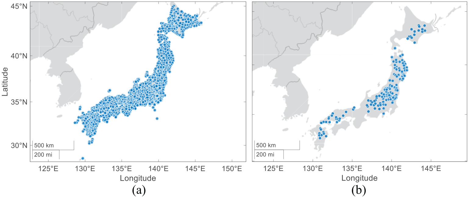
Spatial distribution of the 1725 K-NET and KiK-net recording sites (Japan) used in this study. (a) 1580 training sites. (b) 145 testing sites.

Figure 3.

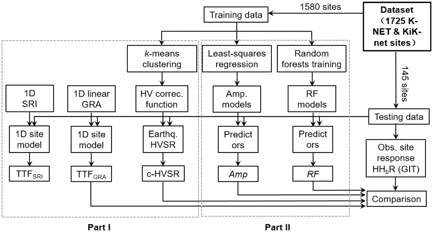
Flowchart illustrating the evaluation of different site-response estimation approaches. SRI—the square-root-impedance method; GRA—1D ground response analysis; c-HVSR—corrected HVSR; Amp—parametric amplification predictive models by least-squares regressions; and RF—random forests (supervised machine learning) models. Ergodic approaches are evaluated in a separate study.

Figure 4.

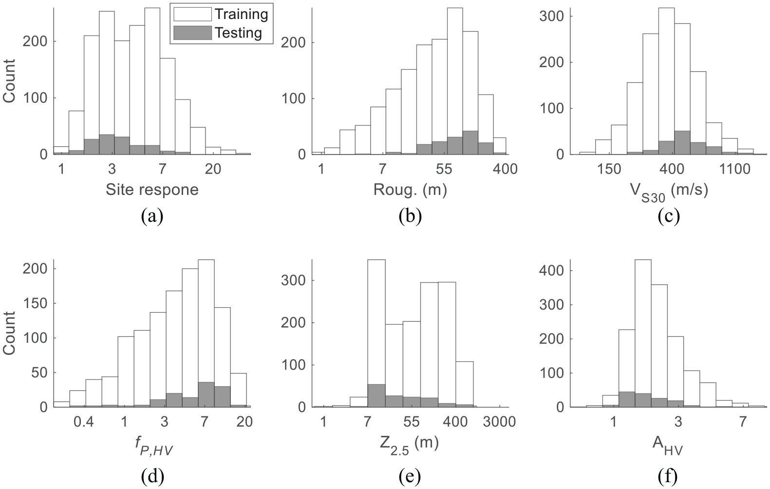
Histograms at the 1580 training and the 145 testing sites. (a) Site responses (from GIT) at f = 1.0 Hz. (b) Topographic roughness. (c) V_S_30. (d) Peak frequency on HVSR (f_{P, HV}). (e) Depth to 2.5 km/s velocity horizon inferred from a 3D velocity model J-SHIS (Z_2.5). (f) Amplitudes of HVSR at f = 1.0 Hz (A_HV). All site parameters are collected from the site database by Zhu et al. (2021b).

Site metadata

Site data, including V_S₃₀, surface geology, topographic roughness (the largest difference in elevation between the target pixel and the surrounding cells on a digital elevation model (DEM)), and geomorphological category, at the 1725 selected sites are collected from an open-source site database developed by Zhu et al. (2021b). We note that in the open site database, V_S₃₀ was only derived for sites at which velocities were logged to a depth reaching or exceeding 30 m (Zhu et al., 2021b). Thus, for sites with borehole depth z < 30 m (e.g. most K-NET sites), we estimate V_S₃₀ from its correlation with V_Sz (average S-wave velocity to z = 20, 15, and 10 m) using the equations established in this study (Figure S1, see Data and Resources). In addition, for the very few sites without V_Sz measurements (no published Vs profiles), we use V_S₃₀ values from the Japan Seismic Hazard Information Station (J-SHIS, see Data and Resources), where V_S₃₀ is inferred from other easy-to-measure proxies, for example, surface geology. Distributions of site proxies at sites in the training and testing databases are presented in Figure 4.

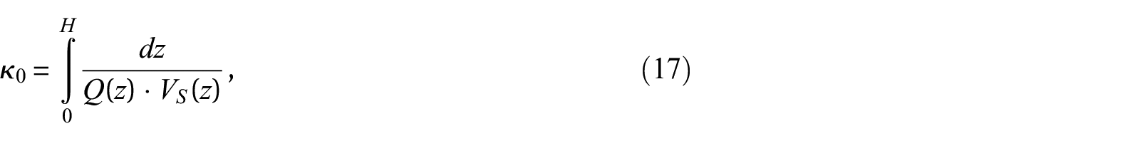
In addition, we also derive the attenuation parameter kappa (κ) at K-NET and KiK-net recording sites (Figure 5a) using the same FAS dataset (Nakano et al., 2015) as described above. The spectra are further smoothed by a Parzen window of 1 Hz length to assure that the high-frequency decay is not influenced by dominant troughs or peaks. κ is computed as the slope of the high-frequency decay of acceleration FAS in 10–25 Hz in log-linear space. Then the κ values of two horizontal components are combined by their geometric mean if their difference is within 10 ms (otherwise rejected). κ is assumed to be a linear function of source-site distance (Anderson and Hough, 1984). The intercept (i.e. zero-distance κ) is denoted as κ₀ which represents the attenuation of seismic waves within the geological structure immediately beneath the site.

Figure 5.

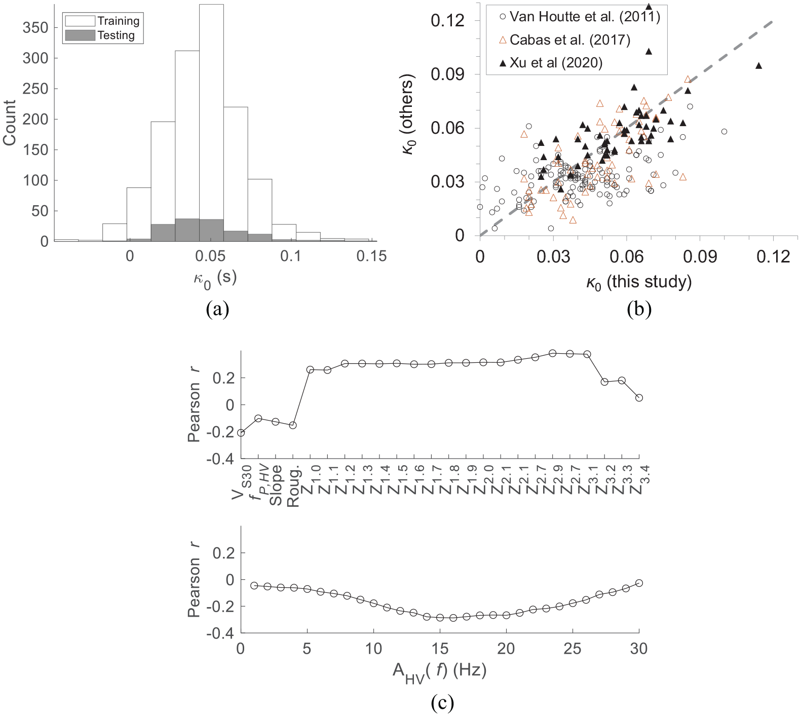
(a) Histograms of kappa (κ₀) values at the 1580 training and the 145 testing sites derived from surface recordings in this study. (b) Comparison of κ₀ from different studies at common sites. (c) Pearson’s correlation of κ₀ with various site parameters and HVSR amplitudes at different frequencies based on the training sites. Z_x (x = 1.0, 1.1, 1.2, ..., 3.4) is from the J-SHIS 3D velocity model which has velocity reversals.

Our κ₀ values are considered to be consistent with those in the literature (Cabas et al., 2017; Van Houtte et al., 2011; Xu et al., 2020) at common sites (Figure 5b). Some deviations are expected since κ₀ results are affected by many factors in the computation (Ktenidou et al., 2013). κ₀ is often used as a site parameter (e.g. Cotton et al., 2006) and it exhibits low correlations with other site parameters examined here (Figure 5c). The strongest correlation is achieved with depth parameters, for example, r = 0.38 for Z_3.1. In this study, we use κ₀ as an attenuation operator in SRI (Boore, 2003; Joyner et al., 1981) and will publish the κ₀ data at K-NET and KiK-net sites in the open-source site database (Zhu et al., 2021b).

Site-specific approaches in site-response estimation

Empirical correction to HVSR (c-HVSR)

For any site on the ground surface, its HVSR can be expressed as:

HVSR (f) = \frac{H (f)}{V (f)} = \frac{H (f)}{H_{b} (f)} \cdot \frac{H_{b} (f)}{V (f)} = \frac{H H_{b} R (f)}{V H_{b} R (f)},

(11)

where $H (f)$ and $V (f)$ represent the geometrical mean of the smoothed FAS of the two horizontal components (NS and EW) and the smoothed FAS of the vertical component (UD), respectively, of a ground motion recorded on the ground surface. Correspondingly, $H_{b} (f)$ is that at the reference rock site, where subscript b denotes outcrop “bedrock” herein, though Zhu et al. (2020c) used the bedrock at depth.

To obtain the site amplification in the horizontal direction, Equation 11 can be rewritten as:

H H_{b} R (f) = HVSR (f) \cdot V H_{b} R (f) .

(12)

Equation 12 indicates that $HVSR (f)$ should be compensated by the vertical amplification $V H_{b} R (f)$ to obtain site amplification in the horizontal direction, $H H_{b} R (f)$ . It is worth noting that the vertical amplification is referenced to the horizontal ground motion at a reference rock site $H_{b} (f)$ , rather than $V_{b} (f)$ . All the three terms in Equation 12 are site-specific. However, a site of interest often lacks a priori information on the site-specific $V H_{b} R (f)$ , which inhibits the direct application of Equation 12 in routine engineering practices. Instead, a generic vertical amplification function $< V H_{b} R (f) >$ averaged over multiple sites (Kawase et al., 2018b) is utilized in Equation 12, and the resultant amplification in the horizontal direction is termed as pseudo-amplification $pH H_{b} R (f)$ , and we refer to this approach as “c-HVSR” in this study:

pH H_{b} R (f) = HVSR (f) \cdot < V H_{b} R (f) > .

(13)

Based on the 1580 training sites, we derive correction spectra $< V H_{b} R (f) >$ (Equation 13) under two different schemes (Table 2). In Scheme I, no clustering is conducted, and the correction spectrum is simply obtained by averaging VH_bRs over all 1580 training sites. In this scheme, no site information is required.

Table 2.

Clustering analysis to VH_bR functions

Scheme	Site proxy	Approach	No. of clusters
I	None	Averaging across all sites	1
II	f_Pv and log₁₀(V_S₃₀)	k-means clustering	5

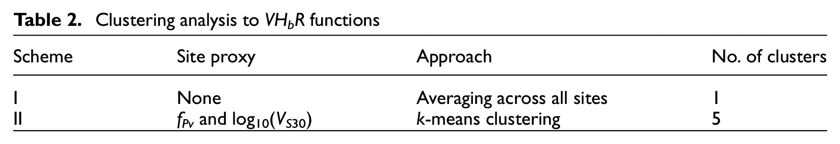
In Scheme II (Table 2), we adopt a similar approach as Zhu et al. (2020c). Under this scheme, each site is characterized by f_Pv and log₁₀V_S₃₀. f_Pv represents the peak frequency on VH_bR and is determined by following an automatic procedure (Zhu et al., 2020a). Among the 1580 sites in the training dataset, 880 stations have their f_Pv identified. Then we utilize an unsupervised machine learning technique, k-means clustering, to partition the 880 stations into k number of mutually exclusive clusters based on a chosen distance metric. K-means clustering needs prior knowledge of the number of clusters. According to the within-cluster sum of distances (Figure 6a), we set the optimal number of clusters k to 5. 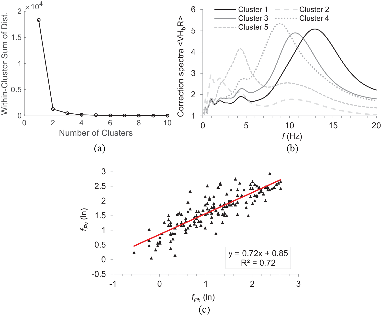The within-cluster mean VH_bR, that is, $< V H_{b} R >$ (Figure 6b), is then taken as the correction function for sites in the corresponding cluster. Subsequently, for a test site with f_Pv and log₁₀V_S₃₀, which existing cluster it belongs to is determined by that of its nearest cluster centroid. In forward applications, if f_Pv is unavailable but there exists the resonant frequency in the horizontal direction (f_Ph), then f_Pv can be estimated from f_Ph using the empirical relationship in Figure 6c. Correction functions for both schemes are provided as supplemental material (Table S1, see Data and Resources).

Figure 6.

(a) Determination of the optimal number of clusters using the within-cluster sum of distances. (b) Generic correction spectra $< V H_{b} R >$ for each cluster. (c) Empirical relationship between f_Ph and f_Pv established using SBSR observations in horizontal and vertical directions at KiK-net sites.

1D outcrop site-response analyses (GRA and SRI)

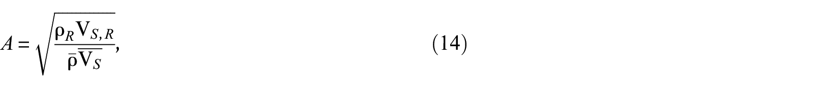
In site-specific seismic hazard evaluations, GRA is widely adopted to assess the effects of surface geology on ground motions. In GRA, the propagation of complex wave fields (P-SV, SH, and surface waves) in 3D media is simplified as the propagation of vertically incident plane SH waves through 1D soil columns (i.e. “1DSH” assumptions). In contrast, SRIs are based on ray theory (Boore, 2003; Joyner et al., 1981) and utilize the QWL velocities and densities to compute attenuated amplifications:

A = \sqrt{\frac{ρ_{R} V_{S, R}}{\bar{ρ} \bar{V_{S}}}},

(14)

where $ρ_{R}$ and $V_{S, R}$ are the density and shear-wave velocity, respectively, at reference depth; $\bar{ρ}$ and ${\bar{V}}_{S}$ are the average density and velocity, respectively, over a depth corresponding to one-quarter of a wavelength for each frequency being considered. SRI can only capture the impedance effects but cannot precisely capture the resonance effects as GRA, thus SRI is a mathematically less exact approach than GRA (Boore, 2013).

For the 145 testing sites, TTFs are computed using both GRA and SRI. For GRA, the software Strata (Kottke et al., 2013) is adopted, whereas the Fortran package site_amp_batch (Boore, 2003) is utilized for SRI. Given the fact that site-response observations are obtained from recordings with PGA ≤ 2.0 m/s² (i.e. linear site responses) with reference to outcrop bedrock (V_S = 3450 m/s), GRA and SRI are thus conducted in the linear domain with the same reference condition, namely outcrop bedrock (V_S = 3450 m/s).

Both GRA and SRI require a 1D physical model, including mass density (ρ), shear-wave velocity (V_S), and damping profiles or κ₀ which govern two competing effects in site responses: amplification and attenuation. Density information is unavailable at the 145 testing sites (KiK-net) and thus is estimated from V_S (Zhu et al., 2020c). Velocity profiles at these sites are established from the boring data published by NIED (2019) and are referred to as the original “V0” profiles (Figure 7a).

Figure 7.

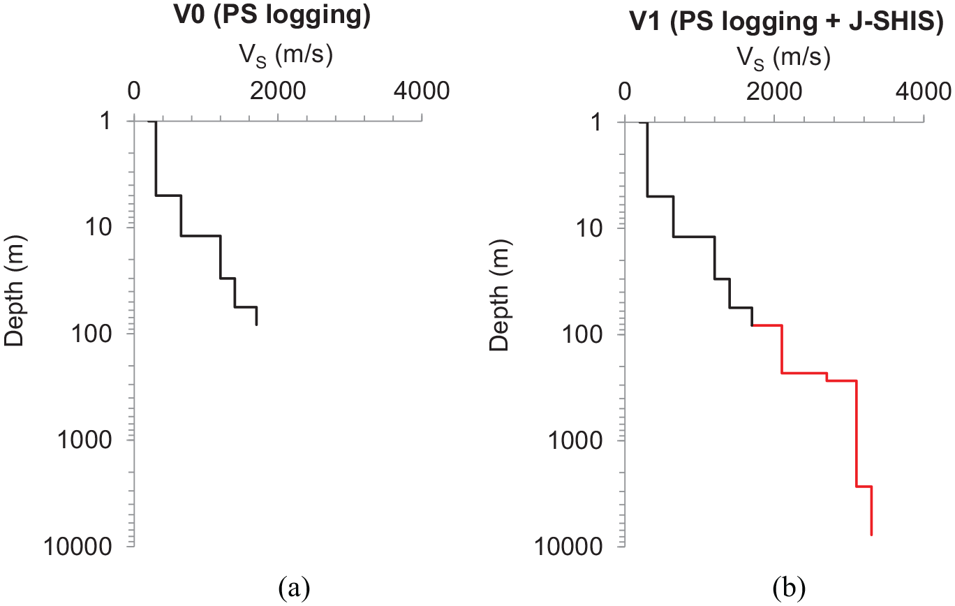
1D velocity profiles for the KiK-net site FKSH06. (a) V0 (PS logging). (b) V1 (PS logging + J-SHIS).

Since KiK-net boreholes do not reach the seismological bedrock (V_S = 3450 m/s), especially for sites in deep sedimentary basins, for example, the Kanto (Tokyo) basin, we thus combine the boring data with velocity structures from the J-SHIS three-dimensional (3D) velocity model, which is developed by NIED (Fujiwara et al., 2012) for the whole of Japan. When combining the two profiles, we give a priority to the KiK-net velocity structure down to the bottom of the boring data, from which to the 3450 m/s V_S horizon we switch to the velocity structure of the J-SHIS model. These composite velocity models are denoted by “V1” profiles (Figure 7b).

Seismologists have long recognized that the amplitude decay of seismic waves within the Earth’s crust, defined herein as the effective attenuation of shear (S) waves, can be approximated by Equation 15 (Anderson and Hough, 1984):

A (r, f) = A_{0} \cdot e^{- π \cdot κ (r) \cdot f},

(15)

where r is distance, f is frequency, and $κ$ is a linear function of distance r (Equation 16) (Anderson and Hough, 1984; Hough and Anderson, 1988):

κ (r) = κ_{0} + κ_{1} \cdot r .

(16)

The slope $κ_{1}$ represents the attenuation due to the horizontal propagation of seismic waves within the crust, and the intercept of $κ_{0}$ represents the attenuation of seismic waves within the geological structure beneath the site and can be expressed as (Campbell, 2009):

κ_{0} = \int_{0}^{H} \frac{dz}{Q (z) \cdot V_{S} (z)},

(17)

where Q is the effective seismic quality factor of S waves. The above equation assumes that the value of Q within the sedimentary column is independent of frequency and represents the combined intrinsic and scattering attenuation.

The value of Q is often estimated from V_S. Campbell (2009) proposed a Q-V_S model (Equation 18) for sites in eastern North America. In this study, we also use this model and refer it to as damping model “D1.” In addition, we also select another Q-V_S relation (Equation 19) established by NIED specifically for Japan. The NIED damping model is available on J-SHIS and is referred to as “D2” in the following.

D1: Campbell (2009) attenuation

Q = 7.17 + 0.0276 \cdot V_{S},

(18)

D2: J-SHIS attenuation model

Q = 40.71 + 0.0725 \cdot V_{S} .

(19)

Comparing D1 and D2 damping models (Figure 8), D1 gives much lower Q estimates (stronger damping) than D2 by a factor of around 3.3. Another widely adopted relation $Q = V_{S} / 10$ (Olsen et al., 2003) gives similar Q values to D2.

Figure 8.

(a) Shear-wave quality factor (Q) models considered in this study, and (b) small-strain damping (D_min) profiles for the KiK-net site FKSH06 with dashed and solid lines corresponding to damping models D1 (Equation 18, Campbell, 2009) and D2 (Equation 19, J-SHIS), respectively.

For GRA, small-strain soil damping (D_min) is required as input and can be derived from Q (Goodman, 1988):

D_{\min} = 1 / (2 \cdot Q) .

(20)

In SRIs, attenuation is accounted for by utilizing $κ_{0}$ as an attenuation operator to un-attenuated amplifications (Equation 14):

e^{- π κ_{0} f},

(21)

where $κ_{0}$ represents the attenuation to seismic waves over the length of the soil column. $κ_{0}$ can be estimated from recordings (Figure 5a) or Q (Equation 17).

Results

Intra-method comparison

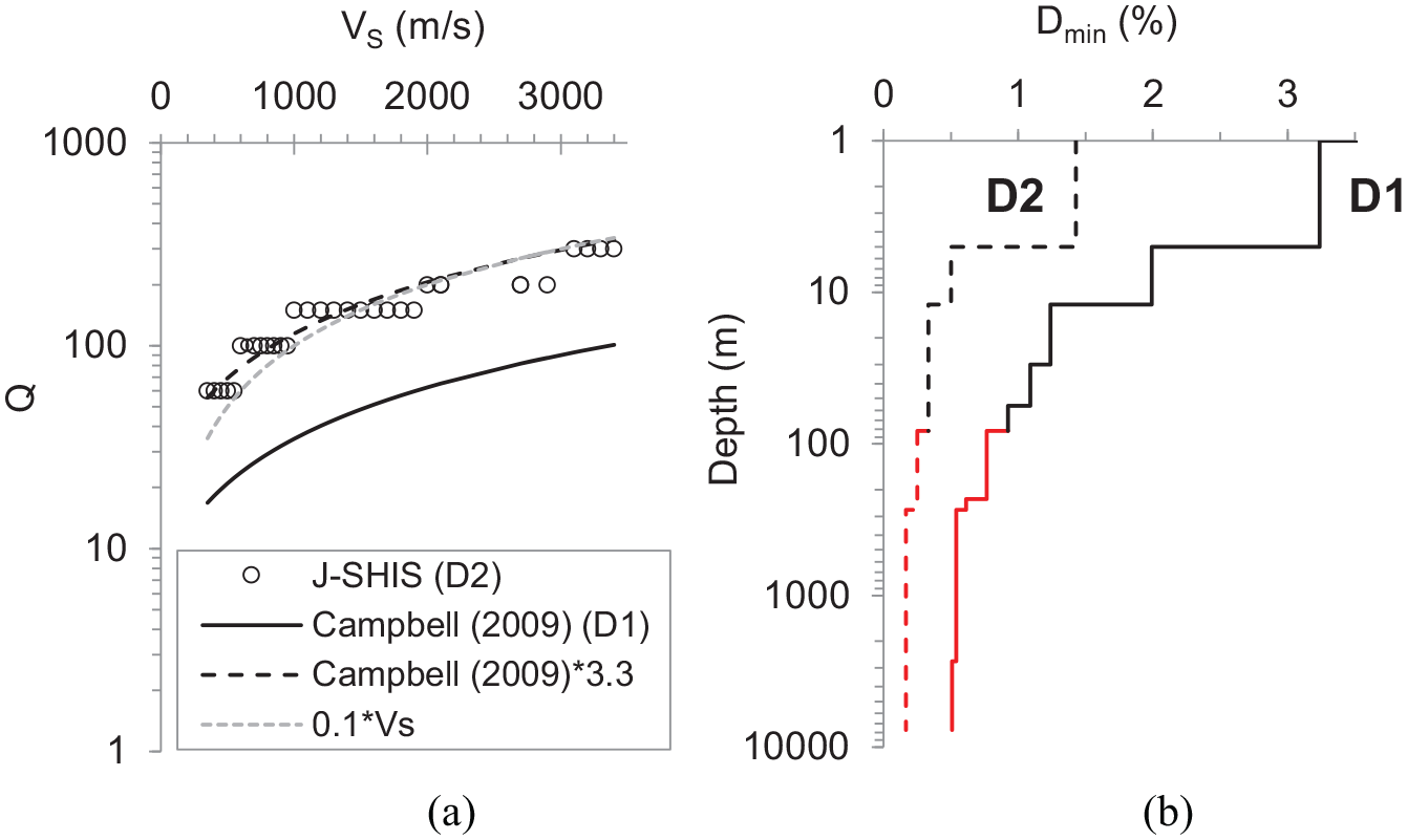
First, we compare the effectiveness of the empirical correction to HVSR (c-HVSR, Equation 13) under two different schemes (Table 2) using the training dataset (1580 sites). In Scheme I, there is only one vertical correction spectrum, and thus site information is not needed. In contrast, there are five correction spectra in Scheme II under which site-specific parameters f_Pv and V_S₃₀ are prerequisites to determine the corresponding correction spectrum. “Scheme I & II” means the mixed use of Scheme I and II in which Scheme II is applied for the sites with site-specific data (i.e. f_Pv or log₁₀V_S₃₀), otherwise Scheme I is utilized. Scheme I and Scheme I & II are applied to all the 1580 training sites, whereas Scheme II is only applied to 880 sites with f_Pv and V_S₃₀.

In terms of standard deviations of residuals between site-response observations (through GIT) and predictions (through c-HVSR under different schemes), Scheme II has the lowest level of dispersion and is followed by Scheme I & II and then Scheme I (Figure 9a). This demonstrates that utilizing site-specific information whenever available will lead to more accurate predictions. Considering both the performance and required input data, we use the combined Scheme I & II hereafter. As an example, c-HVSR is applied to one test site FKSH05 (Figure 9b), and the estimated site response shows a very good match with the observation from GIT.

Figure 9.

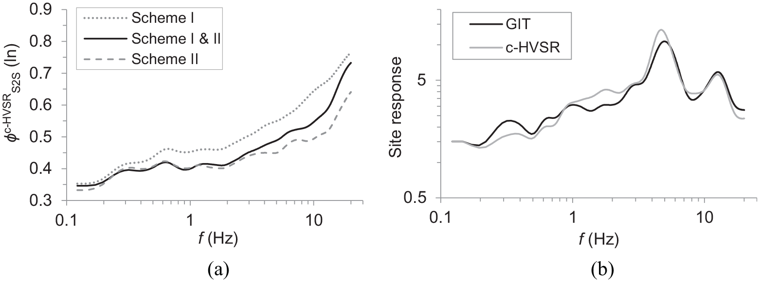
(a) Standard deviation of residuals ( $ϕ_{S 2 S}^{c - HVSR}$ ) between site-response observation (through GIT) and prediction from c-HVSR at the training sites. (b) Site-response estimate from c-HVSR at the test site FKSH05 in comparison with observed site response.

Next, we evaluate GRA predictions using different generic damping models, that is, D1 (Equation 18, Campbell, 2009) and D2 (Equation 19, J-SHIS). We utilize the MAE (Equation 10) between observation and GRA prediction as evaluation criteria. At the 145 testing sites, GRA results using D1 have larger MAE than those using D2 at 92% of the sites (Figure 10a). Considering that D1 gives higher damping values than D2 (Figure 8), the comparison implies that the D1 damping model overpredicts the attenuation effects at sites in Japan. The D1 damping model was initially proposed by Campbell (2009) for sites in eastern North America and may not apply to Japan. GRA and SRI predictions using D2 damping are illustrated for the site FKSH05 (Figure 10b). Both GRA and SRI results still underestimate observed site response in a broad frequency range at this site.

Figure 10.

(a) MAE (Equation 10) of GRA predictions using generic damping models D1 (Equation 18, Campbell, 2009) and D2 (Equation 19, J-SHIS) at each of the 145 testing sites. (b) Site-response predictions from SRI and GRA using D2 damping at the test site FKSH05 in comparison with observed site response through GIT.

Inter-method comparison

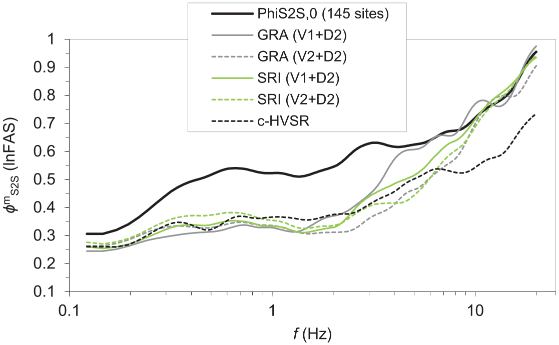
In this section, we evaluate the effectiveness of different approaches (GRA, SRI, and c-HVSR) in reproducing the observed site response (GIT) at the 145 testing sites. We assess the overall performance of a given technique m at the testing sites as a whole, and its performance at the individual sites. The overall performance is measured using the reduction in the standard deviation of residual $ϕ_{S 2 S}^{m}$ (Equation 2) with reference to the standard deviation of full site response HH_bRs (through GIT) at the 145 testing sites, namely $ϕ_{S 2 S}^{0}$ (Equation 5). The reduction reflects the extent to which one approach can capture the site-specificness of site response at sample sites. We note that all approaches are tested on the same dataset in this study, thus $ϕ_{S 2 S}^{0}$ is identical for different techniques (Figure 11). Besides the overall performance of each technique, the efficacy of each approach at individual sites is assessed using three GoF measures (Equation 6–8): Pearson’s r, Spearman’s ρ, and Kendal’s τ (Figure 12 and Table 3). At each site, a “good match” in shape is declared if the GoF metric is larger than 0.6.

Table 3.

Success rates of different methods/models in reproducing observed outcrop site responses at the 145 testing sites

Methods/models	Pearson’s r > 0.6 (%)	Spearman’s ρ > 0.6 (%)	Kendal’s τ > 0.6 (%)
GRA (V1 + D2)	41	40	23
GRA (V2 + D2)	70	66	39
SRI (V1 + D2)	50	48	27
SRI (V2 + D2)	41	49	32
SRI (V1 + κ₀)	71	64	47
c-HVSR	89	85	79

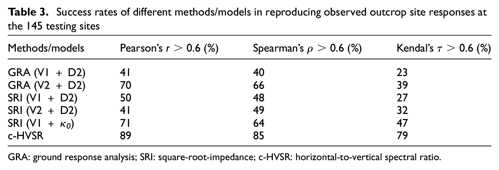
GRA: ground response analysis; SRI: square-root-impedance; c-HVSR: horizontal-to-vertical spectral ratio.

Figure 11.

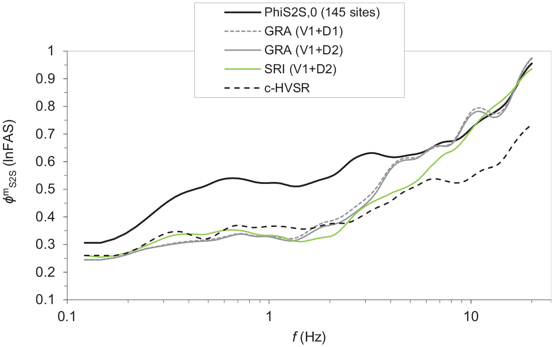
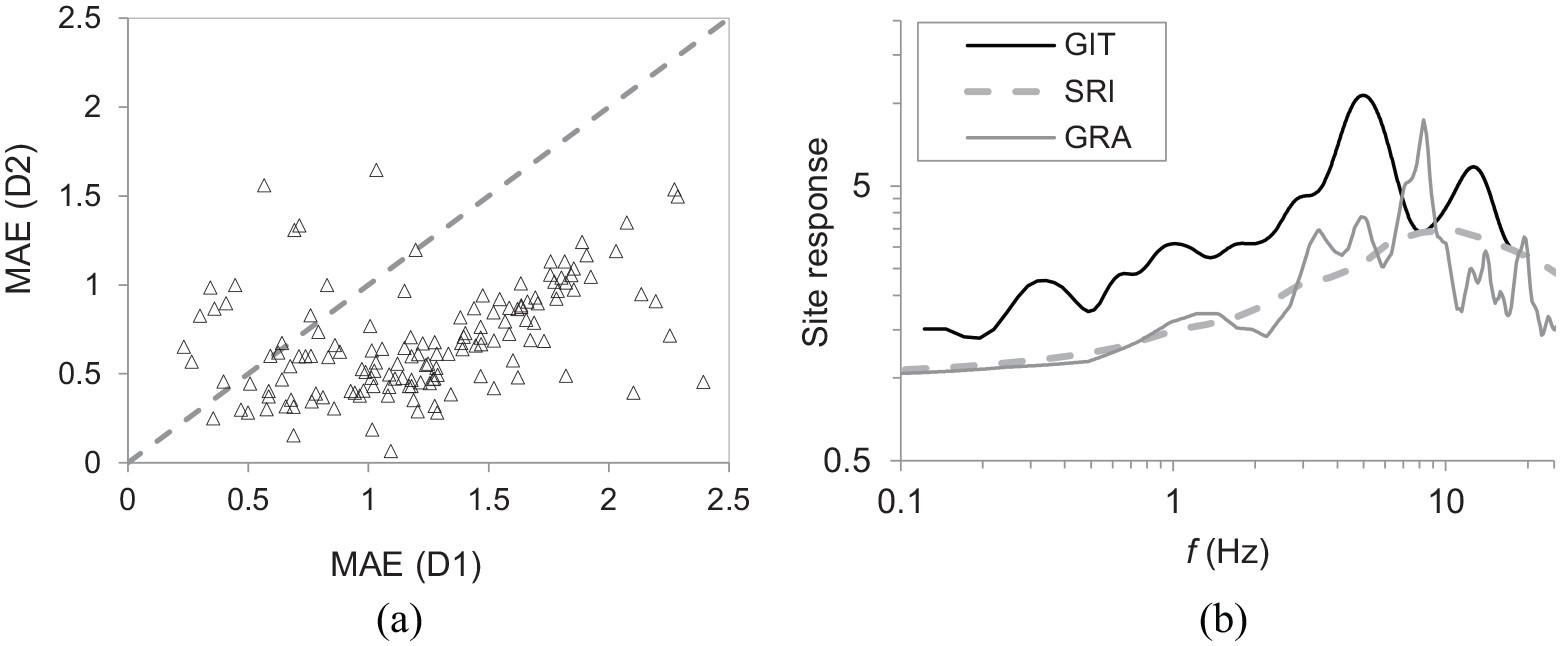
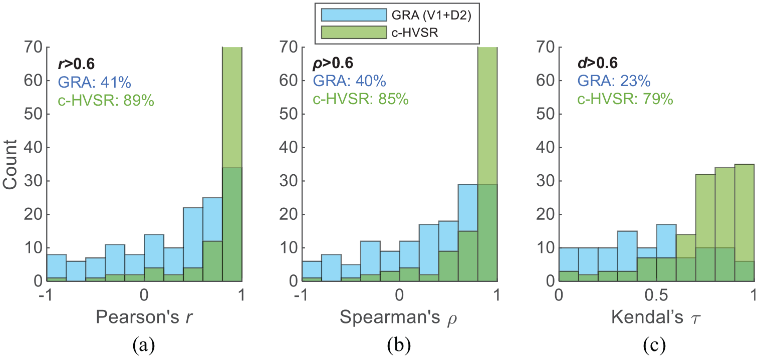
Comparison of the standard deviation of prediction residuals ( $ϕ_{S 2 S}^{m}$ ) of different site-response estimation approaches at the 145 testing sites. Also presented is $ϕ_{S 2 S}^{0}$ for those 145 testing sites.

Figure 12.

Histograms of (a) Pearson’s r, (b) Spearman’s ρ, and (c) Kendal’s τ, between site-response observation (GIT) and predictions (from GRA and c-HVSR) at the 145 testing sites. Each GoF metric is computed in the frequency range between f_{0, TTF} and 20 Hz where f_{0, TTF} is the fundamental resonant frequency on TTF using GRA. Success rates (GoF > 0.6) of each approach are also displayed in each plot.

Generic damping models, that is, D1 (Equation 18, Campbell, 2009) and D2 (Equation 19, J-SHIS), have negligible impacts on $ϕ_{S 2 S}^{GRA}$ (Figure 11). This can be explained by the fact that both damping models are based on V_S profiles and thus capture a similar degree of site-specific attenuation features, resulting in nearly identical standard deviations.

GRA is effective in capturing the site-specific features of site responses at frequencies lower than ∼3.0 Hz but performs poorly at frequencies higher than ∼4.0 Hz (Figure 11). It is known that GRA results should not be utilized for f < f₀ due to the limited length of velocity profiles. In the mid-frequency range ∼0.4–4.0 Hz, $ϕ_{S 2 S}^{GRA}$ is lower than $ϕ_{S 2 S}^{0}$ by ∼0.2 (ln scales). At relatively high frequencies (> ∼4 Hz), the ineffectiveness is because GRA requires finer velocity structures and more accurate site-specific damping estimates, which are critical in modeling the amplification and attenuation of seismic waves at high frequencies.

Comparing SRI with GRA, $ϕ_{S 2 S}^{SRI}$ is lower than $ϕ_{S 2 S}^{GRA}$ by as large as ∼0.1 (ln) in the frequency range between ∼4.0 and ∼7.0 Hz, but at other frequencies, the two are comparable (Figure 11). In addition, SRI achieves good matches in spectral shape at more sites than GRA (Table 3). Thus, SRI exhibits a better overall performance than GRA at the 145 testing sites, which is also reported by Thompson et al. (2011). Mathematically, GRA gives more exact solutions than SRI when the velocity structure used in the computation is accurate. However, since many velocity profiles contain different levels of parametric errors, thus both GRA and SRI predictions are only approximations to observations. However, SRI is insensitive to the details of 1D site models (Boore, 2013), and thus it could perform better than GRA when site models are faulty. However, we will demonstrate, in the following section “HVSR-Consistent Velocity Structure,” that the opposite is true (lower dispersion for GRA than for SRI) when improved V_S structures are utilized.

c-HVSR achieves a better overall performance than both GRA and SRI (Figure 11 and Table 3). $ϕ_{S 2 S}^{c - HVSR}$ is comparable to $ϕ_{S 2 S}^{GRA}$ at frequencies below ∼3 Hz. However, at higher frequencies $ϕ_{S 2 S}^{c - HVSR}$ is lower than $ϕ_{S 2 S}^{GRA}$ . Zhu et al. (2020c) used SBSR as observation and came to the same conclusion. In addition, $ϕ_{S 2 S}^{c - HVSR}$ is also lower than $ϕ_{S 2 S}^{SRI}$ , though the “turning point” is at f = ∼6 Hz (Figure 11). When we examine the efficacy at individual sites, GRA (V1 + D2) achieves a “good match” at 41%, 40%, and 23% of sites using r, ρ, and τ, respectively (Figure 12 and Table 3), whereas c-HVSR achieves a “good match” at 89%, 85%, and 79% of sites. In other words, c-HVSR doubles the success rates of GRA (V1 + D2), which is also consistent with the results of Zhu et al. (2020c) using SBSR as observation.

Using single-station recordings to constrain site models

Besides the simplifications to wave propagations in 1D site-response analyses, another main reason for the poor performance of GRA and SRI is the erroneous or inaccurate velocity and damping profiles. For instance, some of the boring data at KiK-net sites are found to be unable to reproduce the resonant frequencies derived experimentally, for example, using SBSR or HVSR (e.g. Pilz and Cotton, 2019). Besides, accurate characterization of soil attenuation properties is crucial in wave propagation modelings, especially for high-frequency components, but remains a challenge. In the following, we discuss two strategies based on the single-station recordings to potentially improve predictions from 1D site-response analyses: using HVSR-consistent velocity structure and site-specific kappa (κ₀) measurements.

HVSR-consistent velocity structure

HVSR-consistent velocity structures are defined as those of which theoretical HVSR (Kawase et al., 2011) can reproduce the one from earthquake weak-motion recordings. To obtain HVSR-consistent velocity profiles for the 145 testing sites, we invert the complete velocity structures from the ground surface down to the seismological bedrock (3.45 km/s) from HVSR of earthquakes using the program by Nagashima et al. (2014). We utilize the existing V1 velocity structure as a reference model and search for the optimal one using the hybrid heuristic search method. The inversion algorithm only searches among candidate profiles of which velocities are within the ± 50% range of the reference value for shallow portion (from surface to borehole) and thicknesses within the ± 50% range of the reference for the deeper part (borehole to 3.45 km/s).

The HVSR inversion is made to reproduce the observed HVSR by searching for the best values in terms of the S-wave velocity in the boring layer or the thickness in the J-SHIS structure for the whole frequency range of 0.12–20 Hz. Because we use the V1 structure as a reference to determine the searching range, we will get the V1 structure as the resultant structure from the inversion if it is the best, but it is quite unlikely for almost all the sites. Note that the inversion should have a direct constraint to the absolute velocity or thickness values because we use the fixed seismological bedrock velocity and the whole HVSR as spectral amplitudes as evidenced by Nagashima et al. (2014) and Kawase et al. (2018a). These newly inverted V_S structures are referred to as “V2” profiles. As an example, the V2 profile for the same site FKSH06 as shown in Figure 7 is illustrated in Figure 13a. Its corresponding small-strain damping profiles estimated from V_S (Equation 18 and 19) are given in Figure 13b.

Figure 13.

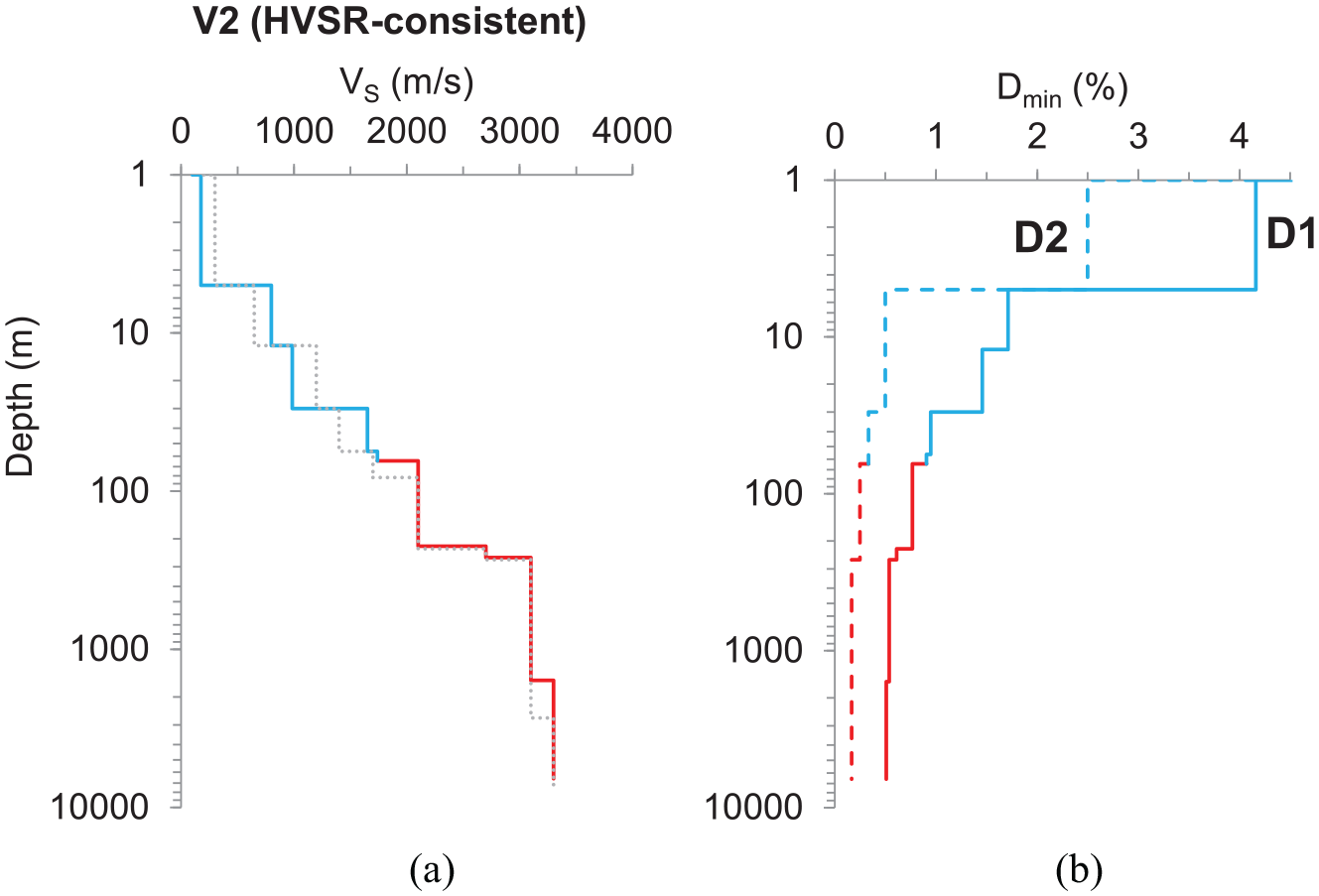
(a) Earthquake HVSR-consistent V_S structure (V2) for the KiK-net site FKSH06 of which the V1 profile (Figure 7b) is also displayed here, and (b) its small-strain damping (D_min) profiles using models D1 (Campbell, 2009) and D2 (J-SHIS), respectively.

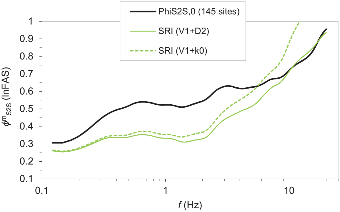
Comparing to V1 profiles, the newly inverted V2 structures results in much lower $ϕ_{S 2 S}^{GRA}$ by as large as 0.16 (ln) in the frequency range from ∼2 to ∼10 Hz (Figure 14), but out of this frequency range, $ϕ_{S 2 S}^{GRA}$ remains nearly unchanged. This demonstrates the benefits of utilizing HVSR-consistent velocity structures in GRA in the mid-to-high frequency range. When we examine the GoF at each site, GRA using V2 can secure a “good match” at 70%, 66%, and 39% of tested sites using r, ρ, and τ, respectively, which are significantly higher than 41%, 40% and 23% using V1 models (Table 3).

Figure 14.

Improvement in GRA and SRI predictions using HVSR-consistent velocity profiles (V2) at the 145 testing sites comparing with those using V1 profiles. The result for c-HVSR is also displayed.

Similarly, improvement can be also achieved in SRI predictions but to a less extent compared with GRA (Figure 14). This can be attributed to the insensitivity of SRI results to model details. In addition, it is interesting to see that utilizing the improved structures (V2), the advantage of SRI over GRA, as observed between ∼4.0 and ∼7.0 Hz when V1 is used (Figure 11), diminishes. If we examine the GoF measures for V2 profiles (Table 3), GRA achieves higher success rates than SRI using all three metrics, indicating GRA results have a better match with observations in shape than SRI predictions. Thus, considering both $ϕ_{S 2 S}^{m}$ and GoF, GRA performs better than SRI when improved structures (V2) are utilized. Therefore, the performance of GRA relative to SRI depends on the quality of velocity structures.

Even if the improved V2 profiles are employed, GRA and SRI predictions, in the aggregate, are still outperformed by c-HVSR (Figure 14 and Table 3). The underperformance of GRA and SRI is due to their ineffectiveness at high frequencies (f > ∼8 Hz), which is primarily attributable to the inaccurate estimation of small-scale velocity variations and attenuation properties in 1D site models.

Site-specific kappa (κ₀) measurements

We then examine the direct use of kappa (κ₀) as an attenuation operator in SRI (Equation 21). κ₀ at each site (Figure 5a) in this study is estimated from surface recordings and thus represents the attenuation effect of the complete geological structure beneath a site. However, κ₀ in SRI (Equation 21) corresponds to the attenuation over the length of the soil column, namely from the ground surface to seismological bedrock (V_S = 3.45 km/s). Thus, the contribution from the structure deeper than 3.45 km/s (κ_0.rock) needs to be separated from surface κ₀ (i.e. κ_{0, surface}):

κ_{0} = κ_{0, surface} - κ_{0, rock},

(22)

where κ_{0, surface} is directly estimated from surface recordings using the approach of Anderson and Hough (1984), but site-specific value for κ_{0, rock} is unavailable and thus is set to κ_0.rock = 0.007 s considering the suggested value for hard-rock sites in other regions (Campbell et al., 2014). Hence, SRI predictions can be obtained using Equations 14, 21, and 22 at the 145 testing sites.

Comparing with the damping model D2 (J-SHIS), SRI results using κ₀ lead to a higher $ϕ_{S 2 S}^{SRI}$ at examined frequencies (Figure 15). This suggests that κ₀-informed damping, albeit from a site-specific procedure, does not improve the closeness in amplitudes between predictions and observations compared with the damping from a generic Q-V_S model (D2). However, it is the opposite when it comes to spectral shape (Table 3). GoF metrics indicate that using κ₀ leads to a better match in spectral shape than D2 damping. This mixed result also suggests that it can be misleading to rely on only a single performance measure.

Figure 15.

Comparison between SRI predictions using site-specific kappa (κ₀) measurements (Figure 5a) and those using κ₀ estimates from Q(V_S) profiles (D2, Equation 19) through Equation 17 at the 145 testing sites.

The lack of reduction in $ϕ_{S 2 S}^{SRI}$ might be due to the absence of site-specific κ_{0, rock} estimates. κ_{0, rock} varies significantly from site to site (e.g. Xu et al., 2020), and thus a constant value for κ_{0, rock} may partially offset the benefits of utilizing site-specific κ_{0, surface} (Equation 22). We note that results may be different if one implements the κ₀-informed damping in GRA which is more physical than a κ₀ operator (Equation 21). For instance, Stewart and Afshari (2020) and Wang (2020) reported that GRA predictions using the κ₀-informed damping led to a slightly lower $ϕ_{S 2 S}^{GRA}$ than those using generic damping models in the mid-frequency range. Nevertheless, the estimation of site-specific $κ_{0}$ needs on-site earthquake recordings with a good distance coverage and is rather susceptible to many factors, for example, ambient noises and resonances at high frequencies. The mixed results on the use of κ₀ entail more work before we could implement κ₀ measurements in site-response analyses.

Discussion

Performance of GRA under within and outcrop conditions

Our results on GRA denote its performance under outcrop boundary conditions (i.e. TTF_out) in predicting observed site responses with reference to motions on outcrop rock (Figure 16a). There exist many studies examining the efficacy of GRA at KiK-net sites (Table 4), but many of these investigations used empirical borehole responses (i.e. SBSR) as targets due to the availability of downhole recordings, and correspondingly TTF from GRA was computed with reference to the motions at borehole bedrock at the base of soil column (i.e. within boundary conditions, TTF_in).

Table 4.

Effectiveness of 1D GRA at KiK-net sites, Japan

GRA	Reference	Observation	V_S and D_min	No. of sites	Good match	Frequency range	Success rate (%)
TTF_out	This study	GIT	V1 + D2	145	r > 0.6	f_{0, TTF} to 20	41
TTF_in (random)	Zhu et al. (2020c)	SBSR	V0 + D1	90	r > 0.6	f_{0, TTF} to 25	27
TTF_in	Zhu et al. (2020c)	SBSR	V0 + D1	90	r > 0.6	f_{0, TTF} to 20	16
TTF_in	Kaklamanos and Bradley (2018)	SBSR	V0 + Optimal D_min	114	r > 0.6	f_{0, TTF} to min(4 f_{0, TTF}, 20)	18
TTF_in	Thompson et al. (2012)	SBSR	V0 + Optimal D_min	100	r > 0.6	f_{0, TTF} to min(4 f_{0, TTF}, 20)	18

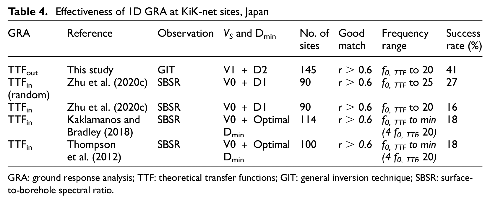
GRA: ground response analysis; TTF: theoretical transfer functions; GIT: general inversion technique; SBSR: surface-to-borehole spectral ratio.

Figure 16.

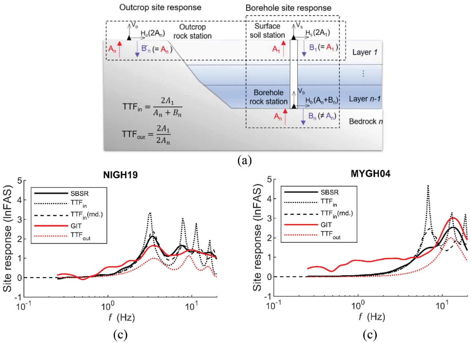
(a) Illustration of borehole and outcrop site responses. A_n and B_n are the amplitudes of up- and downgoing waves, respectively, within bedrock, and A₁ and B₁ are those at the ground surface of soil site. Theoretical borehole (TTF_in) and outcrop (TTF_out) site responses from GRA in comparison with corresponding observations from SBSR (Zhu et al., 2020c) and GIT (Nakano et al., 2015), respectively at sites, (b) NIGH19, and (c) MYGH04. rnd. denotes the average site response over 30 random profiles at a given site. Note SBSR and GIT have different reference conditions.

In practice, outcrop site responses from GRA are needed to adjust the seismic hazards on reference outcrop rock conditions from probabilistic seismic hazard analyses. Thus, it is imperative to check whether GRAs under within and outcrop conditions have similar efficacy; in other words, whether the effectiveness inferred from borehole response analyses applies to outcrop conditions. Herein, we only compiled some results on KiK-net sites, Japan (Table 4) since velocity profiles of other regions may have a different level of parametric uncertainty.

The success rates of GRA borehole responses are lower than that of GRA outcrop responses (Table 4). This can be explained by the fact that GRA borehole responses significantly overpredict the effects of downgoing waves which would be largely scattered by lateral heterogeneities in reality (e.g. Bonilla et al., 2002). As a result, TTF_ins contain significant resonant peaks that either do not exist (i.e. pseudo-resonances, Figure 16b) or are less significant than the peaks on observed borehole responses, that is, SBSR (Figure 16c), as also noted by Tao and Rathje (2020). Thus, TTF_ins have a low success rate in matching SBSR in shape. However, when the effects of downgoing waves on TTF_in are mitigated using 30 random profiles generated by Monte Carlo simulations at each site, Zhu et al. (2020c) realized a higher success rate than using only base-case profiles (Table 4).

One needs to account for the effects of downgoing waves on TTF_ins when inferring the intended effectiveness of GRA (outcrop conditions) from borehole response analyses. Nevertheless, outcrop response analyses (TTF_out vs GIT) should be preferred. Despite the higher success rate of GRA under outcrop conditions than under within conditions, GRA using V1 structures still fails to reproduce the observed site responses at the majority of examined KiK-net sites (Table 4). In another similar study, Pilz and Cotton (2019) excluded sites at which f_{0, TTFs} from GRA are inconsistent with the ones from observations, and then a higher success rate was found among the remaining sites.

Modeling and parametric uncertainties in GRA predictions

The poor performance of GRA is known to be associated with two types of errors: modeling and parametric uncertainties (Toro, 1995). Modeling uncertainty arises because of the simplifications/assumptions to the complex physical process, that is, the 1DSH assumptions. These assumptions are very likely to break down in cases where a site has prominent 2D or 3D features (non-1D) or is significantly affected by surface waves (non-vertical SH incidence). Even if the 1DSH assumptions hold at a site, we are still limited by our ability to perfectly measure all parameters used to define the site model for GRA, especially small-scale variations within sediments, attenuation parameters, and soil nonlinear properties, and these types of error constitute the parametric uncertainty.

Both parametric and modeling uncertainties in GRA results vary from site to site. In site-specific seismic hazard analyses of safety-critical buildings or infrastructure, the parametric uncertainty is accounted for through sensitivity analyses in which input parameters in GRA (e.g. V_S profile) are varied according to a certain statistic distribution (EPRI, 2013). However, the modeling uncertainty in GRA is not explicitly considered (e.g. Rodriguez-Marek et al., 2021). The underestimation resulting from ignoring the modeling uncertainty may be balanced by the fact that the parametric uncertainty might be overestimated by considering the marginal distributions of parameters (e.g. Strasser et al., 2009).

If on-site recordings are available at a site of interest, both types of errors can be constrained:

To reduce the level of parametric uncertainty, preliminary checks on 1D models can be conducted to identify those of which site signatures (e.g. f_{0, TTF}, theoretical HVSR or dispersion curves) are inconsistent with the ones derived empirically. For these sites, more works on site characterization are warranted.

Similarly, to reduce the degree of modeling uncertainty, prior investigations can be carried out to determine whether a target site has subsurface irregularities. This can be achieved using, for instance, the directionality of HVSR (Matsushima et al., 2017), variability of HVSR from different events (HVSR sigma σ_HV,s, Zhu et al., 2021a), or a combination of indicators (Pilz et al., 2021). Then decisions can be made about the suitability of 1D analyses or the necessity of multi-dimensional models.

Furthermore, to mitigate both types of errors simultaneously, Zhu et al. (2021a) suggested a dual-parameter framework: f_{0, TTF}/f_{0, HV} (the ratio of f_{0, TTF} to f_{0, HV}) and σ_HV,s, to constrain parametric and modeling uncertainty, respectively.

All the above strategies entail on-site recordings, but the reduced estimation uncertainties may incentivize stakeholders/practitioners to instrument the target site and collect records in the early planning stage of a safety-critical project.

The match or mismatch between GRA predictions and observations reflects the combined effects of both modeling and parametric uncertainties, which, though conceptually clear, are difficult to separate. We utilize different GoF metrics to quantify the match or mismatch, but we emphasize that a single GoF measure only tells part of the story. For instance, Pearson’s r only measures the strength of association in spectral shapes. Keeping this partiality in mind, we check the dependency of Pearson’s r on various site characterization proxies. For both borehole (Figure 17a to e) and outcrop (Figure S2, see Data and Resources) site responses, Pearson’s r shows some dependence on these site parameters. Softer and flatter sites with less variable HVSR tend to have higher r values (better matches). However, the strength of dependence is not very strong, though it may be worth further exploring their combinations, for example, σ_HV,s and f_{0, HV} (Figure 17f) from single-station recordings.

Figure 17.

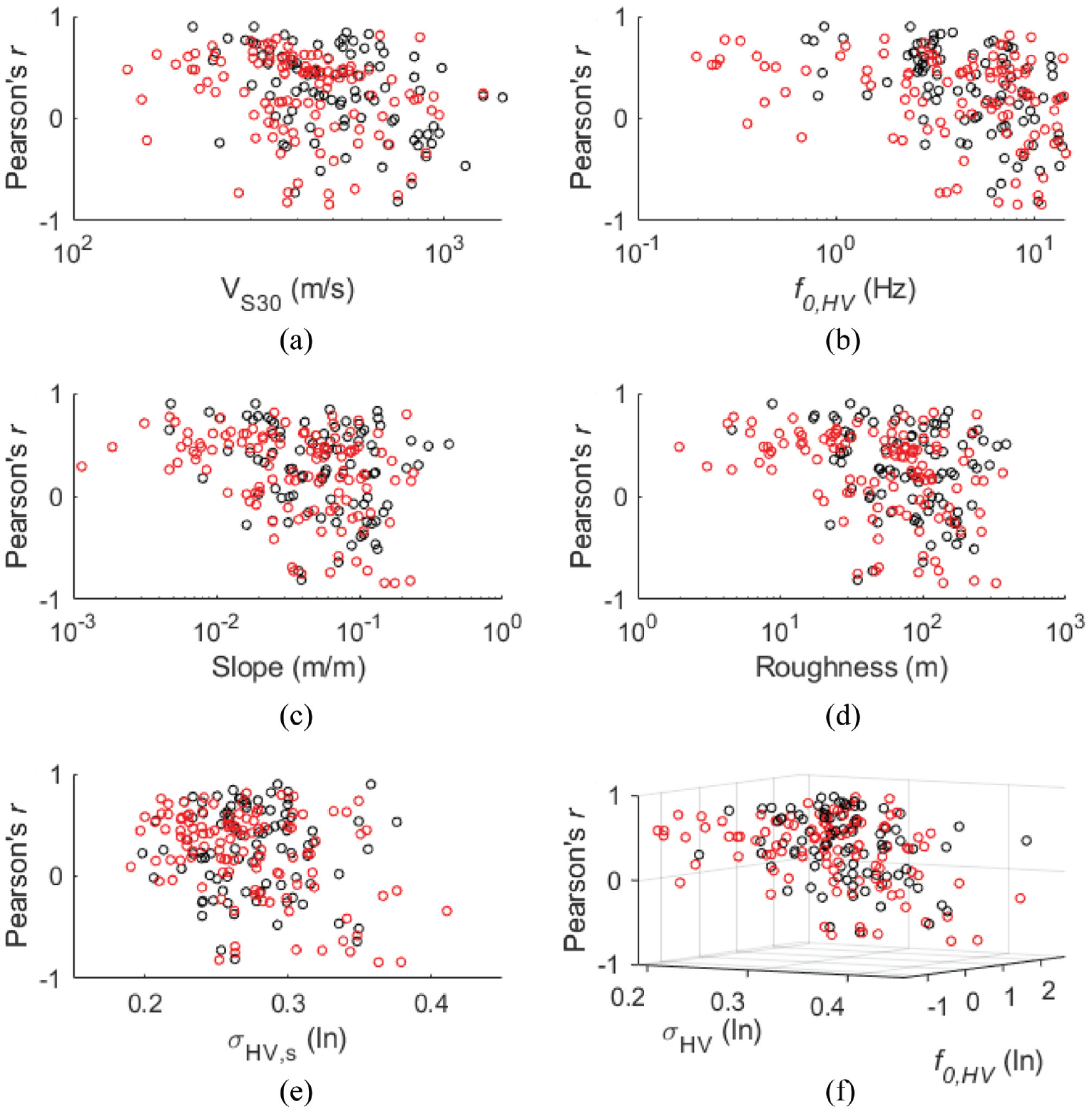
Pearson’s r between SBSR and TTF_in from 1D GRA in the frequency range between f_{0, TTF} and 25 Hz versus various site proxies. (a) V_S_30. (b) f_{0, HV.} (c) Slope gradient. (d) Topographic roughness. (e) σ_HV (ln) averaged over 0.25–25 Hz. (f) σ_HV and f_{0, HV}. Black and red circles represent the results of Zhu et al. (2020c) and Kaklamanos and Bradley (2018), respectively.

Conclusion

To address the question of how well we can predict the average site responses (over many earthquakes) at individual sites, we tested and compared the effectiveness of different estimation techniques using a unique benchmark dataset. The benchmark dataset consists of detailed site metadata (Zhu et al., 2021b) and absolute Fourier outcrop site responses based on observations (Nakano et al., 2015) at 1725 K-NET and KiK-net sites. Evaluated approaches include 1D GRA, the SRI method (also called the QWL approach), the empirical c-HVSR of earthquakes, and regression and machine learning site-response models. The performance of each technique is assessed using the standard deviation of residuals, and GoF in shape, between observations and predictions. The assessment of the regression and machine learning models is presented in a separate paper. In this article, we focus on the evaluation of GRA, SRI, and c-HVSR. Our results show that:

In the aggregate, c-HVSR is very effective in the examined frequency range from 0.1 to 20 Hz and gives significantly more accurate site-response estimates than both GRA and SRI at relatively high frequencies. c-HVSR achieves a “good match” in shape at ∼80%–90% of the 145 testing sites, whereas GRA and SRI fail at most sites.

GRA is effective in capturing site-specific features of site responses at frequencies lower than ∼3.0 Hz but performs poorly at frequencies higher than ∼4.0 Hz. However, the dispersion of GRA predictions can be significantly lowered using ground models inverted from HVSR of weak earthquake motions.

Comparing with generic damping models, utilizing kappa (κ₀) derived from surface recordings as an attenuation operator in SRI realizes a better match in spectral shape but a larger standard deviation of estimation residuals.

These findings suggest that GRA and SRI results have a high level of parametric and/or modeling errors which can be constrained, to a certain extent, by collecting on-site recordings. But additional development is needed in the use of κ₀ to constrain site-specific attenuation properties. c-HVSR is promising in site-specific seismic hazard analyses, and the HVSR correction functions constructed in this study (Table S1, see Data and Resources) can be directly applied to estimate outcrop site responses in Japan. Future studies on developing more site-specific HVSR correction functions and better characterizing site-specific damping profiles are warranted.

Supplemental Material

sj-docx-1-eqs-10.1177_87552930211060859 – Supplemental material for How well can we predict earthquake site response so far? Site-specific approaches

Supplemental material, sj-docx-1-eqs-10.1177_87552930211060859 for How well can we predict earthquake site response so far? Site-specific approaches by Chuanbin Zhu, Fabrice Cotton, Hiroshi Kawase, Annabel Haendel, Marco Pilz and Kenichi Nakano in Earthquake Spectra

Supplemental Material

sj-docx-2-eqs-10.1177_87552930211060859 – Supplemental material for How well can we predict earthquake site response so far? Site-specific approaches

Supplemental material, sj-docx-2-eqs-10.1177_87552930211060859 for How well can we predict earthquake site response so far? Site-specific approaches by Chuanbin Zhu, Fabrice Cotton, Hiroshi Kawase, Annabel Haendel, Marco Pilz and Kenichi Nakano in Earthquake Spectra

Supplemental Material

sj-xlsx-1-eqs-10.1177_87552930211060859 – Supplemental material for How well can we predict earthquake site response so far? Site-specific approaches

Supplemental material, sj-xlsx-1-eqs-10.1177_87552930211060859 for How well can we predict earthquake site response so far? Site-specific approaches by Chuanbin Zhu, Fabrice Cotton, Hiroshi Kawase, Annabel Haendel, Marco Pilz and Kenichi Nakano in Earthquake Spectra

Footnotes

Acknowledgements

The authors thank the National Research Institute for Earth Science and Disaster Prevention (NIED), Japan for making the strong motion and PS logging data available. They also thank three anonymous reviewers who provided very constructive feedback on this work.

Authors Note

Fabrice Cotton is also affiliated from Institute for Earth Sciences, University of Potsdam, Potsdam, Germany.

Declaration of conflicting interests

The author(s) declared no potential conflicts of interest with respect to the research, authorship, and/or publication of this article.

Funding

The author(s) received no financial support for the research, authorship, and/or publication of this article.

ORCID iD

Marco Pilz

Supplemental material

Supplemental material for this article is available online.

Data and resources

Site parameters at K-NET and KiK-net stations used in this study are obtained from an open-source site database https://doi.org/10.5880/GFZ.2.1.2020.006. Seismograms and KiK-net PS logging data (V0 profiles) were downloaded from http://www.kyoshin.bosai.go.jp (profiles were accessed on 5 February 2018). J-SHIS is an integrated online platform developed by NIED for the Probabilistic Seismic Hazard Maps for Japan and various underlying data https://www.j-shis.bosai.go.jp/map/JSHIS2/download.html?lang = en. The Fortran program site_amp_batch for SRI computation is made available by David Boore at www.daveboore.com (last accessed 12 October 2019). The software Strata (Kottke et al., 2013) is used for GRA. Supplemental materials include one table (Table S1) and two figures (Figure S1 and S2). Table S1 tabulates the HVSR correction spectra. Figure S1 displays the relations between V_S₃₀ and V_Sz (z = 10, 15, and 20 m) established in this study. depicts the Pearson’s r between outcrop site-response observation (from GIT) and prediction (from 1D GRA) against various site parameters.

References

Anderson

Hough

(1984) A model for the shape of the Fourier amplitude spectrum of acceleration at high frequencies. Bulletin of the Seismological Society of America 74: 1969–1993.

Bonilla

Steidl

Gariel

Archuleta

(2002) Borehole response studies at the Garner Valley Downhole Array, Southern California. Bulletin of the Seismological Society of America 92: 3165–3179.

Boore

(2003) Prediction of ground motion using the stochastic method. Pure and Applied Geophysics 160: 635–676.

Boore

(2013) The uses and limitations of the square-root-impedance method for computing site amplification. Bulletin of the Seismological Society of America 103: 2356–2368.

Boore

Stewart

Seyhan

Atkinson

(2014) NGAWest2 equations for predicting PGA, PGV, and 5% damped PSA for shallow crustal earthquakes. Earthquake Spectra 30: 1057–1085.

Cabas

Rodriguez-Marek

Bonilla

(2017) Estimation of site-specific kappa (k0)- consistent damping values at KiK-net sites to assess the discrepancy between laboratory-based damping models and observed attenuation (of seismic waves) in the field. Bulletin of the Seismological Society of America 107: 2258–2271.

Campbell

(2009) Estimates of shear-wave q and k0 for unconsolidated and semiconsolidated sediments in Eastern North America. Bulletin of the Seismological Society of America 99: 2365–2392.

Campbell

Hashash

YMA

Kim

Kottke

Rathje

Silva

Stewart

(2014) Reference—rock site conditions for Central and Eastern North America: Part II—Attenuation (Kappa) definition. Report PEER 2014-12. Berkeley, CA: Pacific Earthquake Engineering Research Center, University of California at Berkeley.

Cotton

Scherbaum

Bommer

Bungum

(2006) Criteria for selecting and adjusting ground-motion models for specific target regions: Application to Central Europe and rock sites. Journal of Seismology 10: 137–156.

10.

EPRI (2013) Seismic evaluation guidance: Screening, prioritization and implementation details (SPID) for the resolution of Fukushima near-term task force recommendation 2.1. Seismic. EPRI report no. 1025281, December. Palo Alto, CA: Electrical Power Research Institute.

11.

Fujiwara

Kawai

Aoi

Morikawa

Senna

Azuma

Ooi

Hao

Hasegawa

Maeda

Iwaki

Wakamatsu

Imoto

Okumura

Matsuyama

Narita

. (2012) Some improvements of seismic hazard assessment based on the 2011 Tohoku earthquake. Number 379. Tsukuba, Japan: Technical Note of the National Research Institute for Earth Science and Disaster Prevention.

12.

Goodman

(1988) Chapter 36: Material damping and slip damping. In: Harris

(ed.) Shock and Vibration Handbook. 3rd ed. New York: McGraw Hill, pp. 361–363.

13.

Hassani

Atkinson

(2018) Application of a site-effects model based on peak frequency and average shear-wave velocity to California. Bulletin of the Seismological Society of America 108: 351–357.

14.

Hough

Anderson

(1988) High-frequency spectra observed at Anza, California: Implications of Q structure. Bulletin of the Seismological Society of America 78: 692–707.

15.

Ito

Nakano

Nagashima

Kawase

(2020) A method to directly estimate S-wave site amplification factor from horizontal-to-vertical spectral ratio of earthquakes (eHVSRs). Bulletin of the Seismological Society of America 110: 2892–2911.

16.

Joyner

Warrick

Fumal

(1981) The effect of Quaternary alluvium on strong ground motion in the Coyote Lake, California, earthquake of 1979. Bulletin of the Seismological Society of America 71: 1333–1349.

17.

Kaklamanos

Bradley

(2018) Challenges in predicting seismic site response with 1D analyses: Conclusions from 114 KiK-net vertical seismometer arrays. Bulletin of the Seismological Society of America 108: 2816–2838.

18.

Kawase

Mori

Nagashima

(2018a) Difference of horizontal-to-vertical spectral ratios of observed earthquakes and microtremors and its application to S-wave velocity inversion based on the diffuse field concept. Earth, Planets and Space 70: 1.

19.

Kawase

Nagashima

Nakano

Mori

(2018b) Direct evaluation of S-wave amplification factors from microtremor H/V ratios: Double empirical correction to “Nakamura” method. Soil Dynamics and Earthquake Engineering 126: 105067.

20.

Kawase

Sánchez-Sesma

Matsushima

(2011) The optimal use of horizontal-to-vertical spectral ratios of earthquake motions for velocity inversions based on diffuse-field theory for plane waves. Bulletin of the Seismological Society of America 101: 2001–2014.

21.

Kottke

Wang

Rathje

(2013) Technical Manual for Strata, Geotechnical Engineering Center. Austin, TX: Department of Civil, Architectural, and Environmental Engineering, University of Texas.

22.

Ktenidou

Gélis

Bonilla

(2013) A study on the variability of kappa (κ) in a borehole: Implications of the computation process. Bulletin of the Seismological Society of America 103: 1048–1068.

23.

Kwak

Seyhan

(2020) Two-stage nonlinear site amplification modeling for Japan with VS30 and fundamental frequency dependency. Earthquake Spectra 36: 1359–1385.

24.

Loviknes

Kotha

Cotton

Schorlemmer

(2021) Testing nonlinear amplification factors of ground-motion models. Bulletin of the Seismological Society of America 111: 2121–2137.

25.

Matsushima

Kosaka

Kawase

(2017) Directionally dependent horizontal-to-vertical spectral ratios of microtremors at Onahama, Fukushima, Japan. Earth Planets Space 69: 96.

26.

Nagashima

Matsushima

Kawase Sanchez-Sesma

(2014) Application of horizontal-to-vertical spectral ratios of earthquake ground motions to identify subsurface structures at and around the K-NET site in Tohoku, Japan. Bulletin of the Seismological Society of America 104: 2288–2302.

27.

Nakamura

(2019) What is the Nakamura method? Seismological Research Letters 90: 1437–1443.

28.

Nakano

Matsushima

Kawase

(2015) Statistical properties of strong ground motions from the generalized spectral inversion of data observed by K-NET, KiK-net, and the JMA Shindokei Network in Japan. Bulletin of the Seismological Society of America 105: 2662–2680.

29.

National Research Institute for Earth Science and Disaster Resilience (2019) NIED K-NET, KiK-net, National Research Institute for Earth Science and Disaster Resilience. DOI: 10.17598/NIED.0004.

30.

Olsen

Day

Bradley

(2003) Estimation of Q for Long-Period (>2 sec) Waves in the Los Angeles Basin. Bulletin of the Seismological Society of America 93: 627–638.

31.

Pilz

Cotton

(2019) Does the 1D assumption hold for site response analysis? A study of seismic site responses and implication for ground motion assessment using KiK-net strong-motion data. Earthquake Spectra 35: 883–905.

32.

Pilz

Cotton

Zhu

(2021) Assessing two- and three-dimensional site response from single-station earthquake records. Geophysical Journal International, https://doi.org/10.1093/gji/ggab454

33.

Rodriguez-Marek

Bommer

Youngs

Crespo

Stafford

Bahrampouri

(2021) Capturing epistemic uncertainty in site response. Earthquake Spectra 37: 921–936.

34.

Spearman

(1907) Demonstration of formulæ for true measurement of correlation. American Journal of Psychology 18: 161–169.

35.

Stewart

Afshari

(2020) Epistemic uncertainty in site response as derived from one-dimensional ground response analyses. Journal of Geotechnical & Geoenvironmental Engineering 147. DOI: 10.1061/(ASCE)GT.1943-5606.0002402.

36.

Strasser

Abrahamson

Bommer

(2009) Sigma: Issues, insights, and challenges. Seismological Research Letters 80: 40–56.

37.

Tao

Rathje

(2020) The importance of distinguishing pseudoresonances and outcrop resonances in downhole array data. Bulletin of the Seismological Society of America 110: 288–294.

38.

Thompson

Baise

Kayen

Morgan

Kaklamanos

(2011) Multiscale Site-Response Mapping: ACase Study of Parkfield, California. Bulletin of the Seismological Society of America. 101:1081–1100.

39.

Thompson

Baise

Tanaka

Kayen

(2012) A taxonomy of site response complexity. Soil Dynamics and Earthquake Engineering 41: 32–43.

40.

Toro

(1995) Probabilistic models of site velocity profiles for generic and site-specific ground-motion amplification studies. Technical report no. 779574, 17 November. Upton, NY: Brookhaven National Laboratory.

41.

Van Houtte

Drouet

Cotton

(2011) Analysis of the origins of k (kappa) to compute hard rock to rock adjustment factors for GMPEs. Bulletin of the Seismological Society of America 101: 2926–2941.

42.

Wald

Allen

(2007) Topographic slope as a proxy for seismic site conditions and amplification. Bulletin of the Seismological Society of America 97: 1379–1395.

43.

Wang

(2020) Predictability and repeatability of non-ergodic site response for diverse geological conditions. PhD Thesis, University of California, Los Angeles, CA.

44.

Weatherill

Kotha

Cotton

(2020) Re-thinking site amplification in regional seismic risk assessment. Earthquake Spectra 36: 274–297.

45.

Rathje

Hashash

Stewart

Campbell

Silva

(2020) κ0 for soil sites: Observations from KiK-net sites and their use in constraining small-strain damping profiles for site response analysis. Earthquake Spectra 36: 111–137.

46.

Yong

Hough

Iwahashi

Braverman

(2012) A terrain-based site-conditions map of California with implications for the contiguous United States. Bulletin of the Seismological Society of America 102: 114–128.

47.

Zhu

Cotton

Pilz

(2020a) Detecting site resonant frequency using HVSR: Fourier versus response spectrum and the first versus the highest peak frequency. Bulletin of the Seismological Society of America 110: 427–440.

48.

Zhu

Cotton

Kwak

Kawase

Pilz

(2021a) Within-site variability in earthquake site response. Under Review, Preprint. DOI: 10.13140/RG.2.2.30795.92966.

49.

Zhu

Pilz

Cotton

(2020b) Which is a better proxy, site period or depth to bedrock, in modelling linear site response in addition to the average shear-wave velocity? Bulletin of Earthquake Engineering 18: 797–820.

50.

Zhu

Pilz

Cotton

(2020c) Evaluation of a novel application of earthquake HVSR in site-specific amplification estimation. Soil Dynamics and Earthquake Engineering 139: 106301.

51.

Zhu

Weatherill

Cotton

Pilz

Kwak

Kawase

(2021b) An open-source site database of strong-motion stations in Japan: K-NET and KiK-net (v1.0.0). Earthquake Spectra 37: 2126–2149.

Supplementary Material

Please find the following supplemental material available below.

For Open Access articles published under a Creative Commons License, all supplemental material carries the same license as the article it is associated with.

For non-Open Access articles published, all supplemental material carries a non-exclusive license, and permission requests for re-use of supplemental material or any part of supplemental material shall be sent directly to the copyright owner as specified in the copyright notice associated with the article.

0.00 MB

0.27 MB

0.04 MB

0.12 MB

How well can we predict earthquake site response so far? Site-specific approaches

Abstract

Keywords

Introduction

Evaluation framework

Site-to-site variability ϕ S 2 S m

Goodness-of-fit metrics

Fourier absolute site responses from GIT

Site metadata

Site-specific approaches in site-response estimation

Empirical correction to HVSR (c-HVSR)

1D outcrop site-response analyses (GRA and SRI)

Results

Intra-method comparison

Inter-method comparison

Using single-station recordings to constrain site models

HVSR-consistent velocity structure

Site-specific kappa (κ0) measurements

Discussion

Performance of GRA under within and outcrop conditions

Modeling and parametric uncertainties in GRA predictions

Conclusion

Supplemental Material

sj-docx-1-eqs-10.1177_87552930211060859 – Supplemental material for How well can we predict earthquake site response so far? Site-specific approaches

Supplemental Material

sj-docx-2-eqs-10.1177_87552930211060859 – Supplemental material for How well can we predict earthquake site response so far? Site-specific approaches

Supplemental Material

sj-xlsx-1-eqs-10.1177_87552930211060859 – Supplemental material for How well can we predict earthquake site response so far? Site-specific approaches

Footnotes

Acknowledgements

Authors Note

Declaration of conflicting interests

Funding

ORCID iD

Supplemental material

Data and resources

References

Supplementary Material

Site-to-site variability $ϕ_{S 2 S}^{m}$

Site-specific kappa (κ₀) measurements