Validating alternative methods to account for shallow site effects in hybrid broadband ground-motion simulation of small-magnitude earthquakes in New Zealand

Abstract

Proper incorporation of shallow site effects in hybrid broadband ground-motion simulation is essential to improving predictions at soil sites. This paper validates and compares four methods to account for these effects in the predominantly linear regime, using 1446 ground motions from 213 small-magnitude earthquakes ( $3.5\le M_W\le 5.0$ ) recorded at 38 sites in New Zealand representative of a wide range of soil conditions. These methods require $V_{S30}$ or a shear-wave velocity profile, with the second approach relying on either the square-root-impedance method or the theoretical one-dimensional (SH1D) transfer function. Incorporating shallow site effects with any of the considered methods significantly improves accuracy and precision for several intensity measures, including pseudo-spectral acceleration at short vibration periods. Although the reduction in prediction variability was comparable between methods, the SH1D-based approach showed particular benefits in the case of (1) stiff sites for which the simulation overestimates attenuation effects; (2) relatively stiff sites with high-frequency resonances; (3) relatively soft sites with strong resonances in the intermediate frequency range; and (4) sites with a near-surface predominant frequency lower than the frequency range considered for the application of the $V_{S30}$ -based adjustment. This study shows that the potential prediction improvements obtained by using more advanced site-adjustment methods that incorporate additional site-characterization data are highly dependent on the site characteristics and the quality of the ground-motion simulation in a given region. These findings can help to inform site response method selection in forward applications.

Introduction

Site effects can have a strong influence on the amplitude, frequency content, and duration of ground motion (Kramer and Stewart, 2024), and hence, their proper incorporation is a key aspect to consider when performing hybrid broadband ground-motion simulation (e.g. Graves and Pitarka, 2010; Mai et al., 2010), especially at soil sites. Due to computational constraints and a lack of detailed knowledge of near-surface material properties, shallow site effects are usually not directly modeled in regional-scale ground-motion simulations (some exceptions include Paolucci et al., 2016; Seylabi et al., 2021; Taborda et al., 2012). Instead, they are incorporated through an “uncoupled” approach, where the simulated waveform is adjusted to account for initially unmodeled site effects (e.g. de la Torre et al., 2020; Graves and Pitarka, 2010; Lee et al., 2022; Pilz et al., 2021; Razafindrakoto et al., 2021).

Because of the generally limited site-characterization data available at a given location, this posterior adjustment is usually based on semi-empirical or physics-based approaches that involve certain assumptions and simplifications in the description of the site conditions and wave-propagation phenomena. Kuncar et al. (2025) presented and examined five methods for performing this adjustment, which require different amounts of site-characterization data. Broadly speaking, these methods rely on a combination of some of the following approaches: (1) site-response scaling factors from semi-empirical ground-motion models (GMMs) (e.g. Bayless and Abrahamson, 2019; Campbell and Bozorgnia, 2014), (2) square-root-impedance (SRI) method (Boore, 2013; Joyner et al., 1981), and (3) frequency- or time-domain one-dimensional (1D) site-response analysis (SH1D SRA) (Kramer and Stewart, 2024). In the first approach, the site conditions are described by $V_{S30}$ (30 m time-averaged shear-wave velocity), with potentially other secondary parameters, and the site response is inferred from multiple observations and site-response analyses. Since different sites described by the same $V_{S30}$ can present significant differences in their shear-wave velocity ( $V_S$ ) profiles and other near-surface material properties, inaccurate predictions are expected at sites departing considerably from the average condition represented by the GMM for a particular $V_{S30}$ value (Kamai et al., 2016). Kuncar et al. (2025) also showed that this approach is often inconsistent with the regional ground-motion simulation properties and may double-count deep 3D velocity structure effects. The SRI- and SH1D-based methods are physics-based approaches that use more detailed site-characterization data and can ensure compatibility with the regional ground-motion simulation. However, they are based on a simplified 1D representation of the wave-propagation phenomenon, $V_S$ , and other site properties; with the SRI method modeling impedance and attenuation effects, and SH1D SRA relying on the so-called SH1D assumptions (e.g. Kaklamanos et al., 2013) and also accounting for resonance effects.

As a result of the limitations described above, Kuncar et al. (2025) found considerable method-to-method variability in computed site adjustments for several illustrative examples. Given that these limitations can differently affect the prediction performance of each method at different sites (e.g. at sites for which the SH1D assumptions are more realistic, SH1D SRA should display better performance), a validation of these methods against observations over a wide range of site conditions is essential to inform method selection in forward applications. A key question is whether using more detailed site-characterization data (e.g. a $V_S$ profile vs $V_{S30}$ ) can significantly improve predictions. Numerous studies have evaluated the performance of SH1D SRA using multiple observations from vertical arrays (e.g. Afshari and Stewart, 2019; Kaklamanos et al., 2013; Tao and Rathje, 2020; Thompson et al., 2012) or from surface recordings only (e.g. Bahrampouri and Rodriguez-Marek, 2023; de la Torre et al., 2020; Pilz and Cotton, 2019; Thompson et al., 2011; Zhu et al., 2022). In the aggregate, they have found that SH1D SRA exhibits limited performance at a significant percentage of sites due to uncaptured 3D effects and several sources of parametric and modeling uncertainties. Fewer validation studies have considered the SRI method (e.g. Thompson et al., 2011; Zhu et al., 2022), showing comparable or slightly better performance. Validation of the $V_{S30}$ -based approach in hybrid broadband ground-motion simulations (e.g. de la Torre et al., 2020; Lee et al., 2020, 2022) has shown that it can produce significant overprediction for pseudo-spectral acceleration (SA) at long vibration periods when applied to the low-frequency (LF) simulation component.

Only a few validation studies have evaluated some of the discussed site-response approaches within the context of hybrid broadband ground-motion simulation (e.g. de la Torre et al., 2020; Graves, 2022; Graves and Pitarka, 2010; Lee et al., 2020, 2022; Ojeda et al., 2021; Razafindrakoto et al., 2021; Shi, 2019). Considering this specific context is particularly important when implementing and assessing site-adjustment methods (Kuncar et al., 2025), for example, to avoid double-counting site effects that may already be captured by the simulation. Also, regional simulations can manifest inaccuracies in the modeling of source and path effects, which make the validation of the site-response component more challenging. de la Torre et al. (2020) is considered as the most comprehensive study of this type and one of the few that have used more than one site-adjustment method: it compared a $V_{S30}$ -based site factor derived from the Campbell and Bozorgnia (2014) GMM with an adjustment based on 1D time-domain nonlinear SRA. The study considered 200 ground motions recorded at 20 strong-motion station (SMS) sites in Christchurch (New Zealand), from 11 historical events ( $4.7\le M_W\le 7.1$ ) that induced significant soil nonlinearity. They found that the more sophisticated SH1D-based method only generated significant improvements in a small portion of the sites, which had an exceptionally large site response. However, inaccuracies in the regional simulations (some related to the significant fault rupture complexity of the events considered) likely limited the improvements obtained by this method (de la Torre et al., 2020).

This study presents a comprehensive validation of four methods specifically tailored to account for shallow site effects in hybrid broadband ground-motion simulation (Kuncar et al., 2025). One method only requires $V_{S30}$ and is based on a semi-empirical GMM. The other three methods require a $V_S$ profile and rely on the SRI (two methods) or SH1D approach. The validation considers 1446 ground motions recorded at 38 SMS sites from 213 earthquakes with $3.5\le M_W\le 5.0$ . The use of small magnitude events allows for considering a larger number of ground-motion recordings (e.g. as compared to de la Torre et al., 2020); lowering the uncertainties in the regional-scale simulations due to reduced source modeling complexity (Lee et al., 2022); and reducing the likelihood of significant soil nonlinearity, narrowing the focus of this study to the soil response in the small-to-moderate strain range, as a necessary first step before investigating more complex nonlinear soil responses. The sites considered are located in two broad regions of New Zealand with different geologic and geotechnical features, which allows for assessing these methods for a wide range of conditions. These regions were also selected based on the availability of site-characterization data at multiple stations and the presence of relatively high-quality velocity models. The layout of the paper is as follows: first, the observational and site-characterization data as well as the main regional features are discussed. Next, the methods used for the ground-motion simulation and site adjustments are described; the high-frequency (HF) “normalization factor” is introduced; and the partitioning of the residuals is formulated. Finally, validation results are presented, including a comprehensive assessment of the differences and relative performance of the multiple site-adjustment methods considered.

Strong-motion stations and observational data

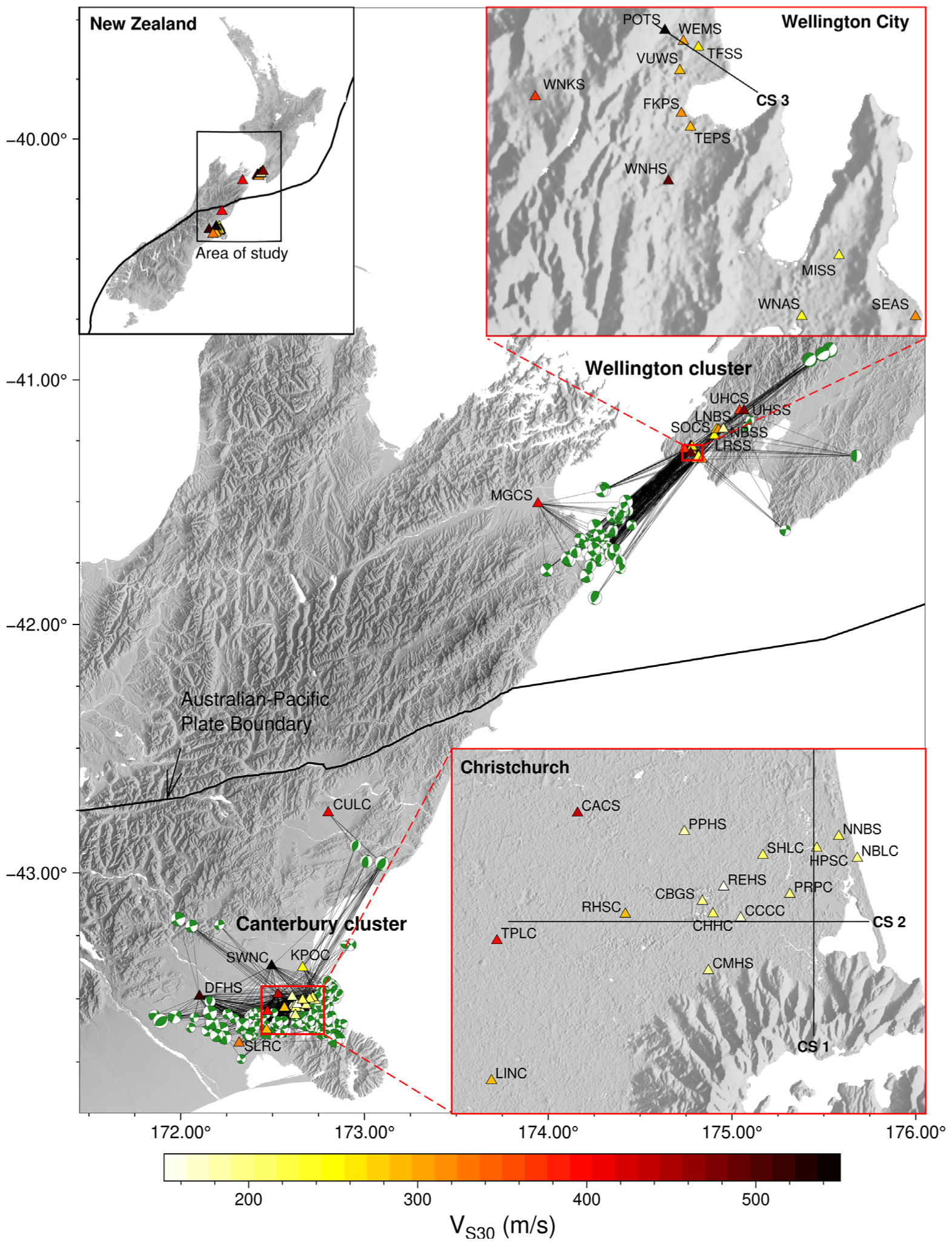
This study uses the observational ground-motion database developed by Lee et al. (2022), which contains active shallow crustal earthquakes with magnitudes $3.5\le M_W\le 5.0$ . In this paper, a high-quality $V_S$ profile was required for the SMSs to be considered. In addition, following Lee et al. (2022), only stations and events with at least three high-quality recordings were included. As a result, a total of 1446 ground motions, recorded at 38 SMS sites and 213 events were considered. Figure 1 shows the spatial distribution of the sites and earthquake sources across New Zealand, which are grouped into two geographic clusters: Canterbury and Wellington. The Canterbury cluster contains 20 sites, most of which are located in the Christchurch metropolitan area, and the Wellington cluster includes 18 sites, 17 of which are distributed across Wellington City and the nearby Hutt Valley further north (the MGCS site is located to the south west in the Blenheim region).

Figure 1.

Distribution of the 38 SMS sites (and the corresponding $V_{S30}$ values) and 213 earthquake sources considered across New Zealand, highlighting the location of the Canterbury and Wellington clusters. Stations are color-coded by $V_{S30}$ . Earthquake sources are shown as green-and-white focal mechanism symbols (“beach balls”), with the symbol size scaled proportionally to the earthquake magnitude. Schematic ray paths corresponding to the 1446 ground motions considered are shown as black lines connecting sources and stations. The location of the cross sections 1 (CS 1), 2 (CS 2), and 3 (CS 3), presented in Figure 3, is shown on the Christchurch and Wellington City insets.

As shown in Supplemental Figure A.1 in Electronic Supplement A, most of the recorded ground motions have a peak ground acceleration (PGA) below $0.1$ g, implying that relatively low levels of soil nonlinearity are expected (e.g. Kaklamanos et al., 2013). However, some stations, mostly with $V_{S30}<220$ m/s, recorded several ground motions with higher PGA, meaning that soil nonlinearity cannot be completely ignored in the site adjustments. In particular, analysis presented in Electronic Supplement A suggests that several sites in the Canterbury cluster could be influenced by soil nonlinearity, but generally to a minor degree.

Site characterization

Site-characterization data used

Site characterization at each of the 38 stations is primarily based on measured $V_S$ profiles (available for all sites), supplemented with borehole, standard penetration test (SPT), cone penetration test (CPT), and microtremor horizontal-to-vertical spectral ratio (mHVSR) data (e.g. Cox and Vantassel, 2018; Deschenes et al., 2018; Stolte et al., 2021; Teague et al., 2018; Wotherspoon et al., 2015), which help constrain or select the most appropriate $V_S$ profile for use in the site-adjustment methods. The data available and used at each site is described in detail in Electronic Supplement B.

While all the sites considered have $V_S$ measurements down to at least 30 m, most of the CPT data available are relatively shallow (as shown in Supplemental Figure B.39 in Electronic Supplement B); for example, CPT data reaching a depth of at least 10 m are only available at 14 sites (37% of the sites included in this study). Considering this, the focus of this paper is on site adjustments that can be applied with only a $V_{S30}$ value or a $V_S$ profile as input. CPT data could be used to constrain nonlinear model parameters for site adjustments involving time-domain site-response analysis (e.g. de la Torre et al., 2020; Kuncar et al., 2025), but given that the expected level of soil nonlinearity is limited in this study, this approach is not considered. The depths of the measured $V_S$ profiles are variable. Most of the profiles in the Christchurch City (e.g. Wotherspoon et al., 2015) are 30 m deep, while for sites west of the city, deep (>1000 m) profiles are available (Deschenes et al., 2018). For most of the sites in Wellington, reliable profiles are available for depths greater than 30 m (e.g. Cox and Vantassel, 2018; Stolte et al., 2021).

Given that alternative sources of site-characterization data are available to constrain the most representative $V_S$ profile at each site (down to the desired depth, corresponding to the main near-surface impedance contrast in each region), including alternative $V_S$ models from surface wave testing, a “best estimate” $V_S$ was heuristically determined at each station. These profiles are presented in Supplemental Figures B.1 to B.38, along with the underlying site-characterization data considered. In most cases, this best estimate is primarily based on surface wave testing. In the case of the NBLC, NNBS, and HPSC sites, located in Christchurch, the profiles determined via surface wave testing were extended down to the Riccarton Gravel unit using the available CPT data along with a Christchurch-specific CPT- $V_S$ correlation (McGann et al., 2015). In Wellington, downhole and seismic CPT (sCPT) data were considered at the POTS, TFSS, WNAS, and MISS sites, and the Hill et al. (2022) basin model was used in some cases (WEMS, TFSS, WNAS, and MISS sites) to extend the profiles down to rock.

Site parameters and regional characteristics

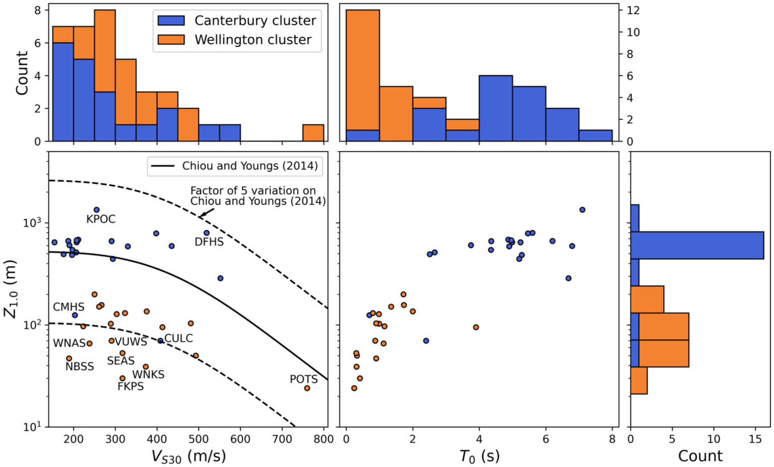
Figure 2 provides the distribution of $V_{S30}$ , $Z_{1.0}$ (depth to the 1 km/s $V_S$ horizon), and $T_0$ (fundamental site period), for the 38 sites considered, disaggregated by cluster. $V_{S30}$ was computed from the best-estimate $V_S$ profiles considered in this study, while $Z_{1.0}$ and $T_0$ are taken from Wotherspoon et al. (2024). Most $Z_{1.0}$ values are inferred rather than constrained by direct measurements, and most of the $T_0$ values were estimated from HVSR measurements or spectral ratio analyses. In some cases, the $V_{S30}$ and $Z_{1.0}$ values provided by Wotherspoon et al. (2024) differ slightly from those computed from the $V_S$ profiles used in this study due to differences in criteria and sources of information (see Supplemental Figure B.40 in Electronic Supplement B). Figure 2 illustrates that the sites in Canterbury have, on average, lower values of $V_{S30}$ than those in Wellington, and higher values of $Z_{1.0}$ and $T_0$ . 79% of the sites characterized by $V_{S30}\le 250$ m/s, and all the sites with $Z_{1.0}\ge 400$ m and $T_0\ge 4$ s, are located in Canterbury.

Figure 2.

$V_{S30}$ , $Z_{1.0}$ , and $T_0$ distributions for the 38 sites considered, disaggregated by cluster. The $V_{S30}$ vs $Z_{1.0}$ plot includes the Chiou and Youngs (2014) $V_{S30}\mathrm{-}{Z}_{1.0}$ correlation for California and non-Japan regions, and boundaries with a factor of five above and below this correlation.

For comparison, Figure 2 displays the Chiou and Youngs (2014) $V_{S30}\mathrm{-}{Z}_{1.0}$ correlation for California and non-Japan regions, based on the NGA-West2 database (Ancheta et al., 2014). Also, in dashed lines, curves with a factor of five above and below this correlation model are presented, allowing for identifying sites that are significantly deeper or shallower, for a given $V_{S30}$ value, than an average site in the NGA-West2 database. All sites in Wellington have $Z_{1.0}$ values falling below the Chiou and Youngs (2014) correlation, with several sites even below the lower factor-of-five boundary. In contrast, most sites in Canterbury have $Z_{1.0}$ values close to or above the Chiou and Youngs (2014) correlation. To better understand these trends, Figure 3 presents three simplified cross-sections (whose locations, in plan view, are indicated in Figure 1) illustrating key geologic features in the Canterbury and Wellington regions, and Figure 4 shows three representative $V_S$ profiles for each cluster.

Figure 3.

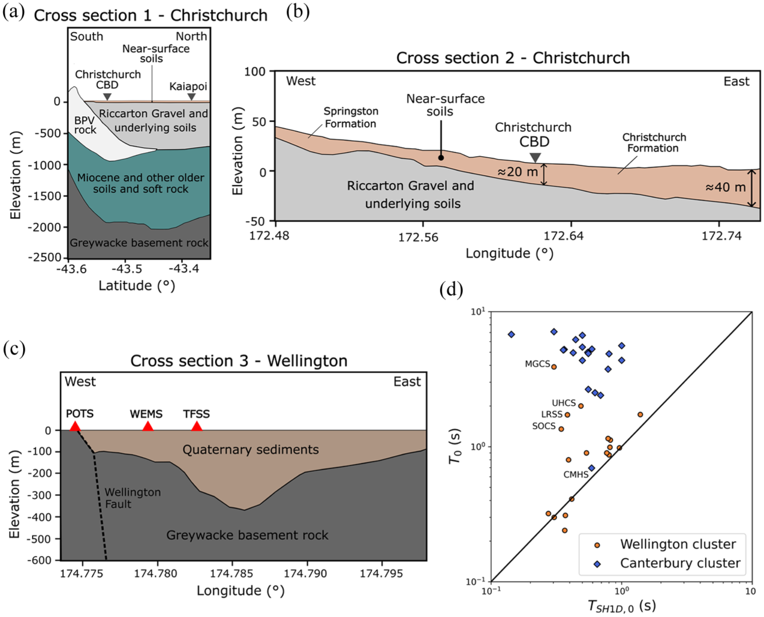
Simplified cross-sections illustrating key geological features in the Canterbury and Wellington regions. (a) Cross section 1: major impedance contrasts beneath the Christchurch metropolitan area (adapted from Lee et al., 2017b; Stolte et al., 2023); (b) Cross section 2: near-surface stratigraphy underlying Christchurch (adapted from Lee et al., 2017a), and (c) Cross section 3: near-surface stratigraphy underlying Wellington (adapted from the Hill et al., 2022 model). (d) Relationship between the $T_{\mathrm{SH}1D,0}$ and $T_0$ values, disaggregated by cluster.

Figure 4.

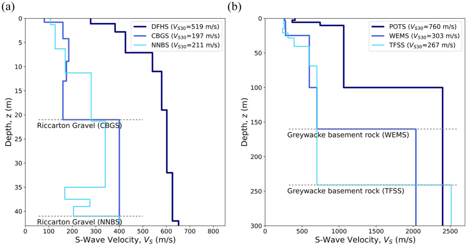
Example $V_S$ profiles for the (a) Canterbury and (b) Wellington clusters. These are the “actual” profiles developed for these sites by combining site-specific data with regional velocity models. The DFHS and POTS sites are characterized by the presence of shallow gravels and rock, respectively (de la Torre et al., 2024a; Deschenes et al., 2018).

Figure 3a illustrates the geologic units that generate the main impedance contrasts beneath the Christchurch metropolitan area, as inferred by Stolte et al. (2023) based on extensive mHVSR data and the 3D Canterbury Velocity Model (Lee et al., 2017b). These are the Riccarton Gravel unit, the Banks Peninsula volcanic (BPV) rock, and the deep greywacke basement rock. Stolte et al. (2023) showed that mHVSR peaks corresponding to the BPV impedance contrasts are generally in the period range 0.5–3 s, and those associated with the basement greywacke rock occur at longer periods (4 + s). Therefore, it is inferred that most of the $T_0$ values presented in Figure 2 for Canterbury correspond to the impedance contrast with the basement rock, typically located at depths greater than 1500 m.

Figure 3b illustrates the surficial stratigraphy beneath Christchurch. On the western side, near-surface soils are associated with the Springston Formation, comprised of alluvial sands and gravels (Teague et al., 2018). In the eastern area of the city, the surficial materials are related to the Christchurch Formation, dominated by Holocene estuarine, lagoon, dune, and coastal swamp deposits of sand, silt, clay, peat, and gravel (Teague et al., 2018). These deposits are characterized by significant spatial variability. For example, near the coast (e.g. NNBS and NBLC sites), the near-surface soils are primarily comprised of dune and beach sands, whereas for the CBGS, CHHC, and CCCC sites, located in the Christchurch CBD, they are dominated by fluvial sands and silts (de la Torre et al., 2020). The relatively soft shallow sediments, mainly associated with the Christchurch Formation, generate a significant impedance contrast with the underlying Riccarton Gravel, which produces mHVSR peaks at periods less than 1 s (Stolte et al., 2023). As illustrated in Figure 3b, the depth to the Riccarton Gravel increases toward the east. Figure 4a shows the $V_S$ profiles at three sites located in the Canterbury Region; from west to east: DFHS, CBGS, and NNBS. The DFHS site, located on the Springston Formation, is characterized by gravels (Deschenes et al., 2018) and exhibits relatively high $V_S$ values, with no significant impedance contrasts near the surface. The CBGS site, in the Christchurch CBD, displays a significant impedance contrast with the Riccarton Gravel at 21 m depth, while the NNBS site, located on the coast, shows this impedance contrast at 41 m depth.

Figure 3c shows that the stratigraphy beneath Wellington is comprised of loose to dense Quaternary sediments deposited on weathered greywacke basement rocks (Hill et al., 2022). The interface between these two units represents the main impedance contrast in the region and, as illustrated in Figure 3c, occurs at relatively shallow depths, with a maximum depth of ≈450 m in the Wellington CBD, and with significant lateral variability (Kaiser et al., 2024). This impedance contrast produces mHVSR peaks in the period range 0.2–2 s in central Wellington (Kaiser et al., 2024). Even though large amounts of geotechnical and geophysical data have been collected (e.g. Cox and Vantassel, 2018; Hill et al., 2022), and gravity surveys have been performed (e.g. Stronach and Stern, 2023), there remains significant uncertainty regarding the depth to the basement rock due to the limited borehole data reaching the basement (Hill et al., 2022; Kaiser et al., 2024). Figure 4b shows the $V_S$ profiles at three sites in Wellington: POTS, WEMS, and TFSS. The approximate location of these sites relative to the Hill et al. (2022) basin model is shown in Figure 3c. POTS is located near the rock outcrop, and therefore, its profile reaches very high $V_S$ values at shallow depths. The WEMS and TFSS sites are located on the Quaternary sediments, at a distance of 340 m from each other. The depth to the basement rock, constrained by the Hill et al. (2022) model, is 160 m and 241 m, respectively, reflecting significant lateral variations. The depth to the basement coincides with $Z_{1.0}$ , which is extensible to most of the sites in this region, explaining the relatively small $Z_{1.0}$ values in Figure 2. The Wellington basin can be subdivided into multiple sub-basins with different geometries and sediment compositions (e.g. de la Torre et al., 2024a).

The above discussion illustrates that significant differences exist between the Canterbury and Wellington clusters regarding their geological features. Particularly, the basement rock is very deep in Canterbury and very shallow in Wellington. Since this study focuses on shallow site effects, the site adjustments in both regions will capture different phenomena. In Christchurch, the site adjustment should be able to account for the near-surface soils and the impedance contrasts with the Riccarton Gravel; whereas in Wellington, it should model the Quaternary sediments and the impedance contrast with the basement rock. In addition to differences in basin characteristics and near-surface layers, the two clusters also exhibit systematic differences in the relative location of seismic sources and stations. Seismic sources in the Canterbury cluster are typically located beneath the modeled Canterbury basin and are relatively shallow. In contrast, seismic sources in the Wellington cluster are generally located outside the modeled Wellington basin, are relatively deep, and typically have larger source-to-site distances than those in Canterbury (see Supplemental Figure A.4 in Electronic Supplement A). This highlights that the two clusters are influenced by very distinct source, path, and site-effect conditions, which may play an important role in the relative performance of different site-adjustment methods.

Methodology

Ground-motion simulation method

This study utilizes physics-based ground-motion simulations performed by Lee et al. (2022) using the hybrid broadband method developed by Graves and Pitarka (2010, 2015, 2016). In this method, a comprehensive 3D physics-based approach is used for the low-frequency (LF) simulation component, and a simplified physics-based approach is adopted for the high-frequency (HF) component. The resulting LF and HF waveforms are then combined using a matched filter, which produces a broadband (BB) ground motion. A LF-HF transition frequency of 1.0 Hz was used in Lee et al. (2022). This value is commonly adopted in previous studies (e.g. Graves and Pitarka, 2010; Razafindrakoto et al., 2021), based on evidence that ground motion can be effectively modeled as a stochastic time series at frequencies above 1.0 Hz (e.g. Hanks and McGuire, 1981). Considering the small magnitude of the events analyzed, a double-couple point source approximation was used in Lee et al. (2022). The LF simulation is based on a kinematic description of the earthquake fault rupture and employs a fourth-order spatial finite-difference algorithm to solve the 3D viscoelastic wave equation. It uses version 2.02 of the New Zealand Velocity Model (NZVM, Thomson et al., 2020), with a grid spacing of 100 m and a minimum $V_S$ of 500 m/s, allowing seismic wave propagation up to 1 Hz (e.g. Baker et al., 2021; Graves and Pitarka, 2010). The HF simulation relies on a stochastic representation of source radiation and a simplified Green’s function that uses a generic 1D $V_S$ structure for the entire country, representative of a basin site. The use of a generic 1D profile, as also adopted in previous studies (e.g. Graves, 2022; Graves and Pitarka, 2010; Razafindrakoto et al., 2018, 2021), is driven by the fundamental inability of the simplified HF simulation approach to account for lateral variations in $V_S$ (e.g. Baker et al., 2021, Ch. 5). Although using site-specific HF 1D $V_S$ profiles is conceptually possible, it would require careful consideration to properly account for the 3D velocity structure, which may vary laterally between the source and site locations. This is beyond the scope of this study. The SRI method (Boore, 2013; Joyner et al., 1981) is used to model impedance effects, while high-frequency spectral decay is captured using a diminution operator based on the site attenuation parameter, ${\kappa }_0$ (Anderson and Hough, 1984), with a generic value of ${\kappa }_0$  = 0.045 s.

Thomson et al. (2020) classified the sedimentary basin subregions included in the NZVM into four types (Type 1 to 4), representing increasing degrees of characterization. In the NZVM v2.02, Wellington is a Type 3 subregion, where the basin geometry is primarily based on boreholes and geophysical surveys, as well as other data sources like SPT and mHVSR. In locations with insufficient data, the sub-surface projection of the topographic slope is considered. More specifically, this subregion utilizes the Semmens et al. (2010) and Boon et al. (2010) models, complemented with the Begg and Johnston (2000) geological map, to constrain the sediment to greywacke bedrock surfaces, along with a generic sediment model. Canterbury is a Type 4 subregion based on detailed geologic and velocity information. This subregion uses a comprehensive basin model (Lee et al., 2017b) based on multiple datasets, including seismic reflection lines, petroleum and water-well logs, cone penetration tests, and geologic maps.

Methods to account for shallow site effects

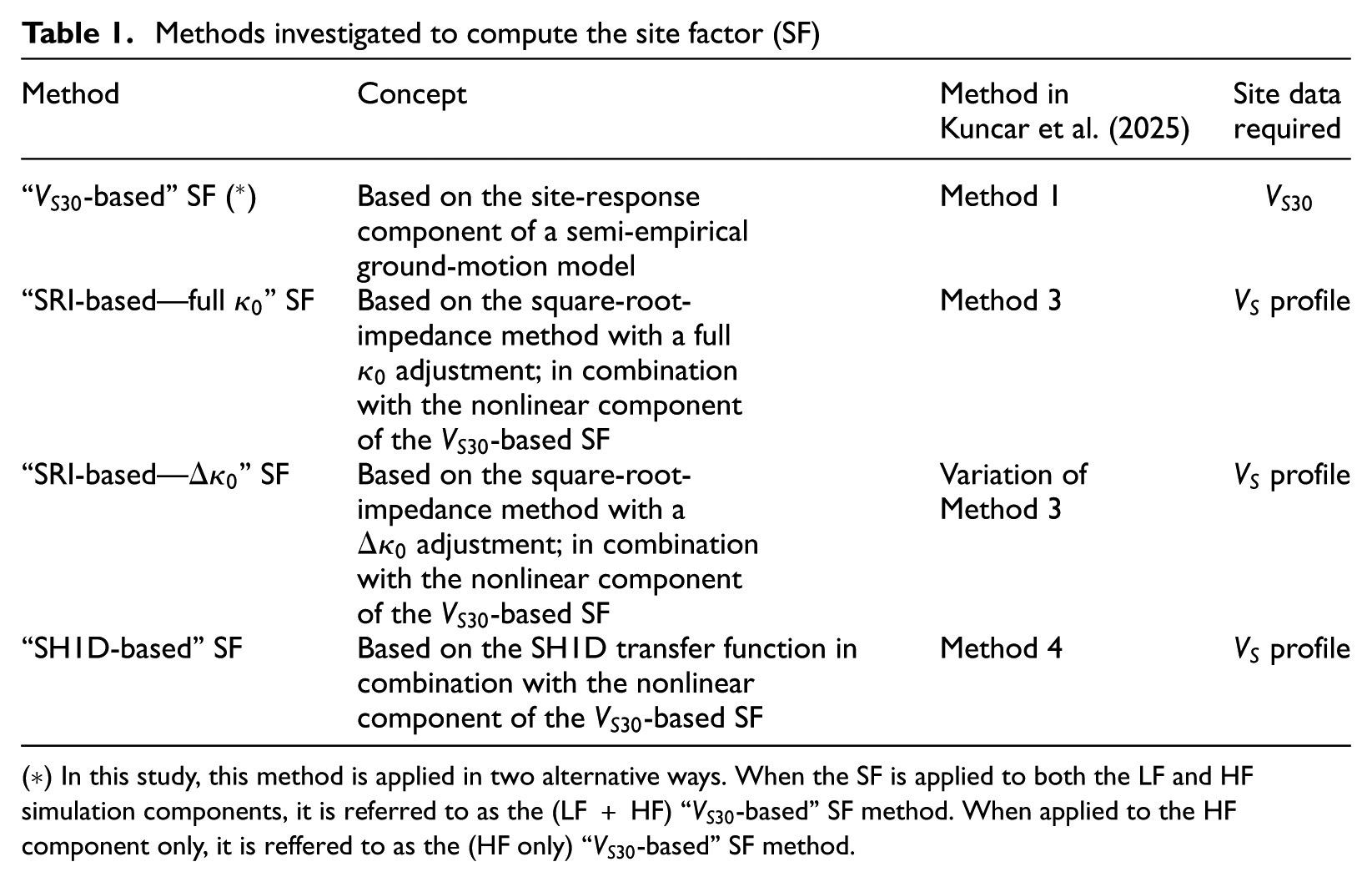
This paper focuses on frequency-domain site adjustments, which consist of the application of a site factor (SF) to the LF and HF waveforms generated through the regional ground-motion simulation, with the aim of obtaining a BB ground motion that includes shallow site effects not captured in the simulation (Kuncar et al., 2025). Table 1 presents the four methods to obtain the SF evaluated in this study. These methods are described and examined in detail in Kuncar et al. (2025), where five approaches were investigated (Methods 1 to 5). Since the focus of this study is on methods that can be used with a site-specific $V_S$ profile, Methods 3 and 4 (including a variation of Method 3) are primarily considered. In addition, the conventional $V_{S30}$ -based Method 1 is included as a reference to evaluate the extent to which a full $V_S$ profile-based adjustment offers improved performance. Since the “ $V_{S30}$ -based” SF method uses a semi-empirical GMM, its linear component is primarily constrained by observations; whereas the other methods approximately model the linear site response through the SRI method or the theoretical SH1D transfer function. All methods use the nonlinear site-response component of existing semi-empirical GMMs to account for the nonlinear site response.

Table 1.

Methods investigated to compute the site factor (SF)

Method	Concept	Method in Kuncar et al. (2025)	Site data required
“ $V_{S30}$ -based” SF (*)	Based on the site-response component of a semi-empirical ground-motion model	Method 1	$V_{S30}$
“SRI-based—full ${\kappa }_0$ ” SF	Based on the square-root- impedance method with a full ${\kappa }_0$ adjustment; in combination with the nonlinear component of the $V_{S30}$ -based SF	Method 3	$V_S$ profile
“SRI-based— $\mathrm{\Delta }{\kappa }_0$ ” SF	Based on the square-root- impedance method with a $\mathrm{\Delta }{\kappa }_0$ adjustment; in combination with the nonlinear component of the $V_{S30}$ -based SF	Variation of Method 3	$V_S$ profile
“SH1D-based” SF	Based on the SH1D transfer function in combination with the nonlinear component of the $V_{S30}$ -based SF	Method 4	$V_S$ profile

(*) In this study, this method is applied in two alternative ways. When the SF is applied to both the LF and HF simulation components, it is referred to as the (LF + HF) “ $V_{S30}$ -based” SF method. When applied to the HF component only, it is reffered to as the (HF only) “ $V_{S30}$ -based” SF method.

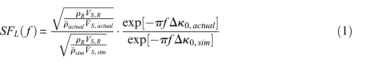
As discussed in Kuncar et al. (2025), the “ $V_{S30}$ -based” SF method is commonly implemented with a truncation at low frequencies (e.g. truncation to a value of 1 for frequencies f < 0.2 Hz, with a taper from f = 0.2–0.5 Hz as considered in Lee et al., 2020), or is applied to the HF component only (e.g. Lee et al., 2022), to avoid overprediction at long vibration periods. Both alternatives are evaluated in this study. Herein, the application of this site factor to both the LF and HF simulation components will be referred to as (LF + HF) “ $V_{S30}$ -based” SF method, and its application to the HF component only as (HF only) “ $V_{S30}$ -based” SF method. In the “SRI-based—full ${\kappa }_0$ ” SF method, the high-frequency site attenuation parameter ( ${\kappa }_0$ ) used in the regional ground-motion simulation (e.g. a generic value of ${\kappa }_{0,\mathrm{sim}}$  = 0.045 s was used in the ground-motion simulations performed by Lee et al., 2022) is replaced by a site-specific ${\kappa }_{0,actual}$ value, which can be estimated, for example, through $V_{S30}$ -based correlations. In contrast, in the “SRI-based— $\Delta {\kappa }_0$ ” SF method, only the portion of ${\kappa }_0$ related to the shallow part of the site ( $\Delta {\kappa }_0$ ), above the half-space considered for the site adjustment, is modified. This second SRI-based approach involves a site attenuation adjustment more consistent with the “SH1D-based” SF method. In this way, the “SRI-based—full ${\kappa }_0$ ” SF adjusts the simulated ground motion for site attenuation effects that can occur over several hundred meters to a few kilometers beneath the site (e.g. Anderson and Hough, 1984; Ktenidou et al., 2015), whereas the “SRI-based— $\mathrm{\Delta }{\kappa }_0$ ” and the “SH1D-based” SFs account only for relatively shallow site attenuation, corresponding to an average depth of ~130 m (with a range of 100–400 m) in this study. The “SRI-based — $\mathrm{\Delta }{\kappa }_0$ ” SF method corresponds to a variation of the “SRI-based— ${\kappa }_0$ ” SF method presented in Kuncar et al. (2025) (see Table 1). The linear “SRI-based— $\mathrm{\Delta }{\kappa }_0$ ” SF is computed as

$$S{F}_L\left(f\right)=\frac{\sqrt{\frac{{\rho }_R{V}_{S,R}}{{\overline{\rho }}_{\mathrm{actual}}{\overline{V}}_{S,\mathrm{actual}}}}}{\sqrt{\frac{{\rho }_R{V}_{S,R}}{{\overline{\rho }}_{\mathrm{sim}}{\overline{V}}_{S,\mathrm{sim}}}}}·\frac{\exp [-\pi f\mathrm{\Delta }{\kappa }_{0,\mathrm{actual}}]}{\exp [-\pi f\mathrm{\Delta }{\kappa }_{0,\mathrm{sim}}]}$$

(1)

where ${\rho }_R$ and $V_{S,R}$ are the soil density and shear-wave velocity, respectively, at the reference condition (i.e. half-space considered); $\overline{\rho }$ and ${\overline{V}}_S$ are the average soil density and travel-time weighted average Vs, respectively, computed at each frequency f (considering a depth equivalent to one-quarter of the wavelength), and the subscript actual and sim represent the “actual” and “simulation” conditions (further explained below); and $\mathrm{\Delta }{\kappa }_{0,\mathrm{actual}}$ and $\mathrm{\Delta }{\kappa }_{0,\mathrm{sim}}$ are the corresponding $\mathrm{\Delta }{\kappa }_0$ values, estimated for each condition. It is worth noting that if $\mathrm{\Delta }{\kappa }_{0,\mathrm{actual}}$ is small compared to $\mathrm{\Delta }{\kappa }_{0,\mathrm{sim}}$ , the attenuation component of this site factor will generate high-frequency amplification rather than deamplification. An example of this behavior is shown in Figure 11, for the SWNC site. Similar formulas for the other three site-adjustment methods are provided in Kuncar et al. (2025).

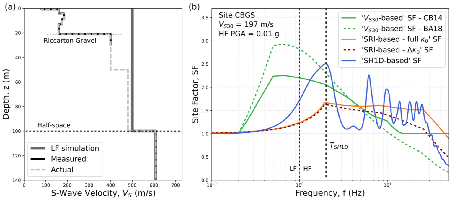
Figure 5 compares the four methods, as implemented in this study, for the CBGS site. Similar figures for all 38 sites are provided in Electronic Supplement C. Figure 5a illustrates the “measured,”“actual,” and LF “simulation” profiles for CBGS, and the half-space considered for the $V_S$ profile-based methods, where the “actual” and LF “simulation” profiles merge. The “measured” profile is determined through site investigation, as explained in the “Site characterization data used” section. The “actual” profile uses the “measured” profile, and if required, combines it with a regional velocity model (e.g. Hill et al., 2022; Thomson et al., 2020) to extend it down to the half-space. The “simulation” profile is the profile considered in the simulation. For the LF simulation component, this profile is extracted from the NZVM v2.02 at the location of interest, enforcing a grid-spacing of 100 m and a minimum $V_S$ of 500 m/s to reproduce the LF simulation conditions; and for the HF simulation, the generic HF profile is used. The depth of the “actual” profile must be sufficient to capture any significant impedance contrast in the shallow subsurface. Figure 5a shows that the “actual” profile for CBGS captures the impedance contrasts with the Riccarton Gravel, which was not modeled in the regional simulation (as observed in the simulation profile). Figure 5b presents the resulting site factors for the different methods, for a representative simulation HF PGA of $0.01$ g, illustrating significant method-to-method variability.

Figure 5.

(a) $V_S$ profiles considered in the computation of the $V_S$ profile-based SFs for the CBGS site, and (2) comparison of the site factors obtained with the different methods, considering a HF PGA of 0.01g. The HF component of the $V_S$ profile-based SFs is presented with the HF normalization factor (introduced in the next section) applied, although this factor has no observable effect at this site.

The “ $V_{S30}$ -based” SF is computed using the response spectra-based CB14 (Campbell and Bozorgnia, 2014) model and the Fourier spectra-based BA18 (Bayless and Abrahamson, 2019) model. The $V_{S30}$ - ${\kappa }_0$ correlation utilized by Bayless and Abrahamson (2019) is used to estimate ${\kappa }_0$ in the “SRI-based—full ${\kappa }_0$ ” SF; and the “Model 1” $V_S$ -Q correlation by Campbell (2009) is used to estimate the quality factor (Q) of the top portion of the actual and simulation profiles, which is then used to compute $\mathrm{\Delta }{\kappa }_0$ and damping ( $D_{\min }$ ) in the “SRI-based— $\mathrm{\Delta }{\kappa }_0$ ” and “SH1D-based” SF methods, respectively (Kuncar et al., 2025). It should be noted that although $V_S$ is constrained using site-specific data in this study, it can still exhibit considerable uncertainty (e.g. Rodriguez-Marek et al., 2021). The use of global $V_S$ -based correlations to estimate attenuation parameters introduces significant additional uncertainty into these estimates (e.g. Ktenidou et al., 2014). Figure 5b also shows the predominant frequency of the near-surface soil profile ( $f_{\mathrm{SH}1D,0}$ ), which is estimated based on the lowest frequency peak in the “SH1D-based” SF. Figure 3d directly compares $T_{\mathrm{SH}1D,0}$ (= $1/f_{\mathrm{SH}1D,0}$ ) and $T_0$ for all 38 sites considered, and shows that in most cases $T_0>T_{\mathrm{SH}1D,0}$ for the Canterbury cluster, illustrating the shallow nature of the SH1D-based adjustment relative to the basement rock depth. In Wellington, the two parameters are in better agreement, showing that in most cases the “SH1D-based” SF captures the impedance contrasts with the underlying rock.

HF simulation profile “normalization factor”

The computation and application of the site factor is performed separately for the LF and HF waveforms for consistency with how the regional-scale hybrid broadband simulation is computed (Kuncar et al., 2025). Since the LF and HF simulation components are obtained using different approaches, the implicit “simulation” profiles in each component may also differ (as explained before, the LF simulation profile is based on the NZVM whereas the HF simulation profile is generic). These differences between the LF and HF “simulation” profiles may lead to inconsistencies in the computation of the SF for the $V_S$ profile-based methods. Since these methods require merging the “actual” and “simulation” profiles at a reference depth (half-space), different “simulation” profiles for LF and HF may also result in different “actual profiles,” reference values, and site factors for the two frequency ranges.

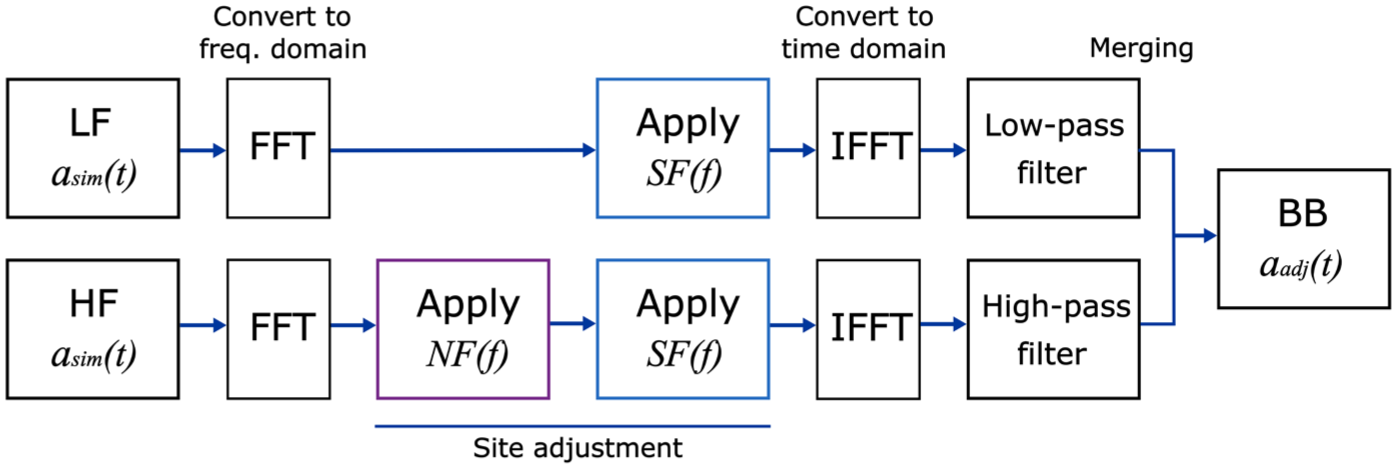
To deal with this issue, a HF “normalization factor” (NF) is proposed in this article. The aim of the NF is to modify the HF waveform such that it represents the ground motion that would have resulted from considering the location-specific LF “simulation” profile instead of the generic HF “simulation” profile in the computation of the impedance-based HF amplification. As shown in Figure 6, the NF is applied to the HF simulated waveform before the site factor, which allows for considering the same “actual” profile, “simulation” profile (corresponding to the LF “simulation” profile), and reference values at the half-space for the LF and HF components, and consequently, the same SF.

Figure 6.

Workflow for the application of the site adjustment for the $V_S$ profile-based methods, including the normalization factor (NF). In this figure, FFT and IFFT correspond to the Fast Fourier Transform and inverse Fast Fourier Transform algorithms, respectively. BB $a_{\mathrm{adj}}\left(t\right)$ is the adjusted broadband acceleration time series that results from the site adjustment.

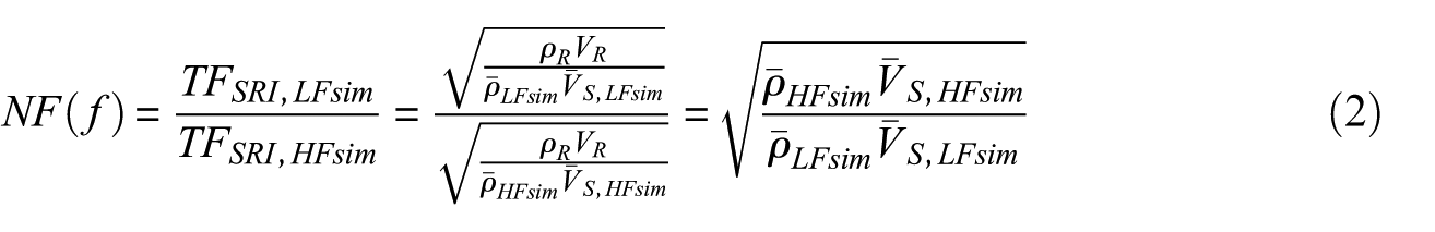
Consistently with the HF simulation methodology (Graves and Pitarka, 2010), the normalization factor is computed using the SRI method, as follows:

$$\mathrm{NF}\left(f\right)=\frac{T{F}_{\mathrm{SRI},\mathrm{LFsim}}}{T{F}_{\mathrm{SRI},\mathrm{HFsim}}}=\frac{\sqrt{\frac{{\rho }_R{V}_R}{{\overline{\rho }}_{\mathrm{LFsim}}{\overline{V}}_{S,\mathrm{LFsim}}}}}{\sqrt{\frac{{\rho }_R{V}_R}{{\overline{\rho }}_{\mathrm{HFsim}}{\overline{V}}_{S,\mathrm{HFsim}}}}}=\sqrt{\frac{{\overline{\rho }}_{\mathrm{HFsim}}{\overline{V}}_{S,\mathrm{HFsim}}}{{\overline{\rho }}_{\mathrm{LFsim}}{\overline{V}}_{S,\mathrm{LFsim}}}}$$

(2)

where $T{F}_{\mathrm{SRI},\mathrm{LFsim}}$ and $T{F}_{\mathrm{SRI},\mathrm{HFsim}}$ are the impedance-based transfer functions for the LF and HF “simulation” profiles, respectively, relative to a reference soil density ( ${\rho }_R$ ) and shear-wave velocity ( $V_{S,R}$ ); $\overline{\rho }$ and $\overline{V_S}$ are the average ρ and travel-time weighted average $V_S$ , respectively, computed at each frequency, f, considering a depth equivalent to one-quarter of the wavelength. The subscripts LFsim and HFsim represent the values associated with the LF and HF simulations, respectively. The above expression assumes that $V_{S,R}$ and ${\rho }_R$ are common for the LF and HF components. Since this normalization factor is purely based on impedance effects, the HF attenuation parameter, ${\kappa }_0$ , remains the same. Also, the HF simulation profile is still used in the “SRI-based— $\mathrm{\Delta }{\kappa }_0$ ” and “SH1D-based” SF methods to remove the near-surface HF attenuation introduced by the simulation (i.e. to compute the simulation $\mathrm{\Delta }{\kappa }_0$ ). This criterion assumes that the generic ${\kappa }_0=0.045$ s used in the HF simulation is associated with the generic HF simulation profile.

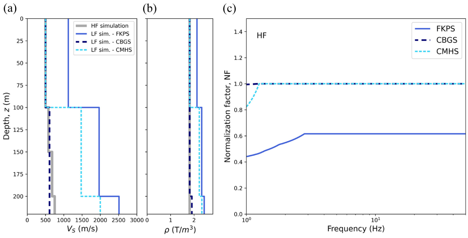
Figure 7 presents the LF and HF “simulation” $V_S$ and ρ profiles for the CBGS, CMHS, and FKPS sites, and the corresponding NFs. Both CBGS and CMHS have the same $V_S$ and ρ values for the LF and HF “simulation” profiles in the top 100 m. Between 100 and 200 m depth, the LF “simulation” $V_S$ profile of CBGS differs only slightly from its HF counterpart; while for CMHS, a substantial increase in the LF simulation $V_S$ and ρ values occurs, generating a significant difference with the corresponding HF “simulation” profiles. In the case of the FKPS site, the differences between the LF and HF “simulation” profiles are even greater and manifest from the surface; for example, the top layer in the HF “simulation” profile has a $V_S=500$ m/s, whereas the LF “simulation” profile has a $V_S\approx 1124$ m/s.

Figure 7.

“Simulation” (a) $V_S$ and (b) ρ profiles, and (c) the resulting normalization factors, for the sites CBGS, CMHS, and FKPS.

Figure 7c presents the resulting normalization factors for the three sites. Since NF is only applied to the HF component, the results are presented only for this frequency range. In the case of CBGS, since the LF and HF “simulation” profiles are almost the same, the NF is close to unity over the entire HF frequency range. For CMHS, $\mathrm{NF}=1$ for $f>1.25$ Hz, reflecting that the top 100 m layer is the same for the LF and HF simulation components. However, NF decreases at lower frequencies due to the differences between the LF and HF “simulation profiles” at greater depths. In the case of FKPS, NF is significantly lower than unity over the entire HF frequency range. Supplemental Figure E.1 in Electronic Supplement E contrasts the effect of NF on the site adjustment for the CMHS and FKPS sites. In this study, 55.3% of the sites display a behavior similar to the CBGS site, 26.3% similar to CMHS, and 18.4% similar to FKPS, and therefore, only a relatively small proportion of the sites are significantly affected by NF over the entire HF frequency range. The application of the proposed normalization factor was required in this study due to the utilization of a generic HF simulation profile in the regional ground-motion simulations used. Alternatively, the same issue could be directly addressed in future studies through the adoption of location-specific HF “simulation” profiles.

Prediction residual partitioning

To consider the entire database of ground motions in the validation of the different methods and to assess systematic prediction effects, a residual analysis is performed. For a given intensity measure (IM), the prediction residual ( ${\mathrm{\Delta }}_{\mathrm{es}}$ ) for the event e recorded at the site s, is defined as

$${\mathrm{\Delta }}_{\mathrm{es}}=\ln {\left(I{M}_{\mathrm{obs}}\right)}_{\mathrm{es}}-{\left(I{M}_{\mathrm{sim}}\right)}_{\mathrm{es}}$$

(3)

where $\ln {\left(I{M}_{\mathrm{obs}}\right)}_{\mathrm{es}}$ and $\ln {\left(I{M}_{\mathrm{sim}}\right)}_{\mathrm{es}}$ are the natural logarithms of the observed and simulated IMs, respectively. The residual ${\mathrm{\Delta }}_{\mathrm{es}}$ is computed for each of the alternative site-adjustment methods considered, where $\ln {\left(I{M}_{\mathrm{sim}}\right)}_{\mathrm{es}}$ is calculated from the site-adjusted simulated waveform (including the HF normalization factor, if applicable). Using a crossed linear mixed-effects regression algorithm (Bates et al., 2015; Stafford, 2014), this residual can be partitioned into the different components of ground-motion variability (Atik et al., 2010), as follows:

$${\mathrm{\Delta }}_{\mathrm{es}}=a+\delta S2S_s+\delta B_e+\delta W_{\mathrm{es}}^0$$

(4)

where a is the (global) model prediction bias and represents the residual fixed effect; $\delta S2S_s$ is the systematic site-to-site residual for the site s; $\delta B_e$ is the between-event residual for the event e; and $\delta W_{\mathrm{es}}^0$ is the “remaining” within-event residual for the event e recorded at the site s, which represents factors that are not systematically captured by a, $\delta S2S_s$ , and $\delta B_e$ .

Noting that the sites and events considered in this paper are grouped into two clusters (Canterbury and Wellington), ${\mathrm{\Delta }}_{\mathrm{es}}$ can be further decomposed as follows:

$${\Delta }_{\mathrm{es}}=a+(\delta C2C_{\mathrm{sc}}+\delta S2S_s^0)+(\delta C2C_{\mathrm{ec}}+\delta B_e^0)+\delta W_{\mathrm{es}}^0$$

(5)

where $\delta C2C_{\mathrm{sc}}$ is the systematic cluster-to-cluster site residual for the site cluster sc and $\delta C2C_{\mathrm{ec}}$ the systematic cluster-to-cluster event residual for the event cluster ec; and $\delta S2S_s^0$ and $\delta B_e^0$ are the “remaining” systematic between-event and site-to-site residuals, respectively, after removing the cluster-to-cluster systematic effects. Since all events belonging to a cluster are recorded only at stations included in the same cluster (Figure 1), this expression can be simplified as

$${\mathrm{\Delta }}_{\mathrm{es}}=a+\delta C2C_c+\delta S2S_s^0+\delta B_e^0+\delta W_{\mathrm{es}}^0$$

(6)

where $\delta C2C_c$ is the total systematic cluster-to-cluster residual for the cluster c (i.e. $\delta C2C_c=\delta C2C_{\mathrm{sc}}+\delta C2S_{\mathrm{ec}}$ ). The sum ( $a+\delta C2C_c+\delta S2S_s^0$ ) is herein referred to as the systematic residual at the site s, and represents the addition of global, cluster, and site systematic residuals. Assuming that $\delta C2C_c$ , $\delta S2S_s^0$ , $\delta B_e^0$ , and $\delta W_{\mathrm{es}}^0$ are independent and normally distributed random variables, with zero mean and variances of ${\varphi }_{C2C}^2$ , ${\varphi }_{S2S_0}^2$ , ${\tau }_0^2$ , and ${\varphi }_{\mathrm{ss}}^2$ , respectively, the total variance ( ${\sigma }^2)$ can be expressed as

$${\sigma }^2={\varphi }_{C2C}^2+{\varphi }_{S2S_0}^2+{\tau }_0^2+{\varphi }_{\mathrm{ss}}^2$$

(7)

The IMs considered in this article are: 5%-damped pseudo-spectral accelerations (SA) for 200 vibration periods logarithmically spaced between 0.01 and 10 s; peak ground acceleration (PGA); peak ground velocity (PGV); cumulative absolute velocity (CAV); Arias intensity (AI); and $5\%-75\%$ and $5\%-95\%$ significant durations ( $D_{s575}$ and $D_{s579}$ , respectively). These IMs are computed from the two horizontal components and are combined using the geometric mean. Although vertical ground motion can be relevant in certain engineering applications (e.g. Taslimi et al., 2024), it was beyond the scope of this study.

Results

This section presents and discusses the main results of the validation study. First, the global model prediction bias and site-to-site variability for the different methods considered are compared. Then, residuals are investigated for a subset of stiff soil and rock sites, and subsequently, for a subset of relatively soft sites. Finally, an alternative method for validating the modeling of shallow site effects based on the site response relative to a nearby reference station is used for five Wellington sites.

Model prediction bias and site-to-site variability

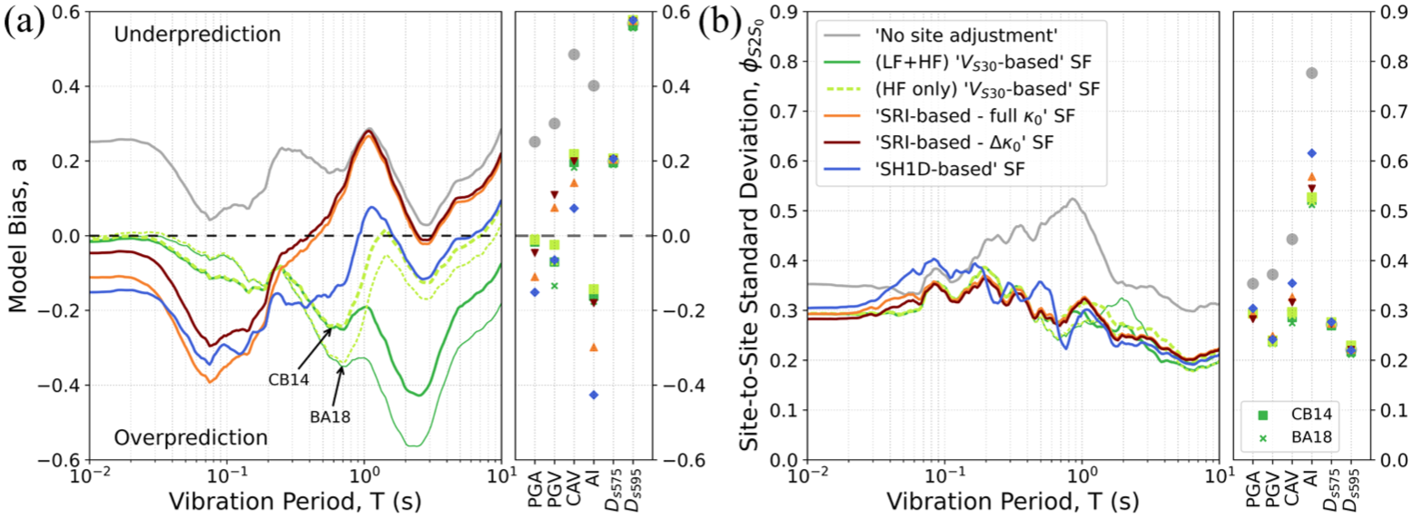
Figure 8 presents the model bias, a, and site-to-site standard deviation, ${\varphi }_{S2S_0}$ , for SA and the other IMs considered. In addition to the four site-adjustment methods investigated, Figure 8 also displays the “no site adjustment” results, which corresponds to the BB ground motions generated by merging the LF and HF simulated waveforms before applying any site adjustment. Hence, this result allows better assessment of the effects of the different SFs from the four methods investigated. Figure 8a shows that the “no site adjustment” simulation underpredicts all IMs considered. The “ $V_{S30}$ -based” SF method significantly reduces the model bias for PGA, PGV, CAV, and SA at $T<0.05$ s, but produces considerable overprediction for AI and SA at longer periods. The (LF + HF) “ $V_{S30}$ -based” SF application generates strong SA overprediction at $T>1$ s, which is more significant for the BA18 model; whereas the (HF only) “ $V_{S30}$ -based” SF application substantially improves prediction bias in this period range. This suggests that deep 3D effects are generally accounted for in the LF simulations for Canterbury and Wellington. The SRI-based SF methods only modify the “no site adjustment” SA bias at $T<0.8$ s, and result in more overprediction than the “ $V_{S30}$ -based” SF approach at $T<0.2$ s, and less overprediction for $T=0.2-0.4$ s. The “SRI-based—full ${\kappa }_0$ ” SF method produces slightly more negative SA model bias than the “SRI-based— $\Delta {\kappa }_0$ ” SF method, which also manifests in other IMs, such as AI. The “SH1D-based” SF method exhibits a similar SA model bias to the SRI-based approaches at $T<0.2$ s, but at $T>0.3$ s it follows a trend more similar to the (HF only) “ $V_{S30}$ -based” SF method, although improving predictions relative to this method for $T=0.4-0.9$ s.

Figure 8.

(a) Model prediction bias, a, and (b) site-to-site standard deviation, ${\varphi }_{S2S_0}$ , for the entire dataset considered, for SA, PGA, PGV, CAV, AI, $D_{s575}$ , and $D_{s595}$ .

For AI, all SFs, and particularly the “SH1D-based” and “SRI-based—full ${\kappa }_0$ ” SF methods, produce overprediction. This can be explained by the substantial overprediction at high frequencies produced by these methods and the strong correlation between AI and high-frequency ground-motion amplitudes (e.g. Bradley, 2015). Both significant durations, $D_{s575}$ and particularly $D_{s595}$ , are underpredicted with all methods, which may be due to wave propagation effects not captured by the LF simulation due to the adopted 3D velocity model (Lee et al., 2022; Pinilla-Ramos et al., 2024), and limitations in the path duration model used in the HF simulation (Lee et al., 2022). Lee et al. (2022) speculated that more comprehensive modeling of near-surface site response may improve significant duration prediction at soft sites for small-magnitude events. However, Figure 8a illustrates that different site adjustments considered in this study have no material effect on the significant duration underprediction. Increasing the near-surface realism of the 3D velocity model, for example by introducing stochastic fluctuations (e.g. Paolucci et al., 2021), may help improve predictions of significant duration.

Figure 8b shows that all site adjustments investigated considerably reduce ${\varphi }_{S2S_0}$ for PGA, PGV, CAV, AI, $\mathrm{SA}(T<0.03s)$ , and $\mathrm{SA}(T>0.2s)$ , relative to the “no site adjustment” case. This reduction is particularly significant at $T=0.4-1$ s, which corresponds to the period range of most of the near-surface predominant periods, $T_{\mathrm{SH}1D,0}$ (Figure 3d). The site-to-site standard deviation for the four methods considered is comparable for all IMs, with the “SH1D-based” SF method exhibiting slightly higher prediction variability for some IMs. This illustrates that the use of more advanced site-response approaches (e.g. the SH1D-based method versus the $V_{S30}$ -based method) does not directly translate into an overall improvement in simulation precision. This can be explained by the recognized modeling limitations of the SRI- and SH1D-based methods, such as the simplified representation of site conditions and wave propagation phenomena through a 1D profile, and parametric uncertainties involved in the site adjustments and regional simulation (e.g. Bahrampouri and Rodriguez-Marek, 2023; de la Torre et al., 2020; Rodriguez-Marek et al., 2021; Thompson et al., 2011, 2012; Zhu et al., 2022). In addition, the relatively shallow site-specific data available at most sites may limit the effectiveness of these site-adjustment methods in improving predictions. Finally, it should be noted that the site-to-site variability reflects simulation precision across all sites, which may mask prediction improvements at individual stations (e.g. different sites may display improvements at different vibration periods).

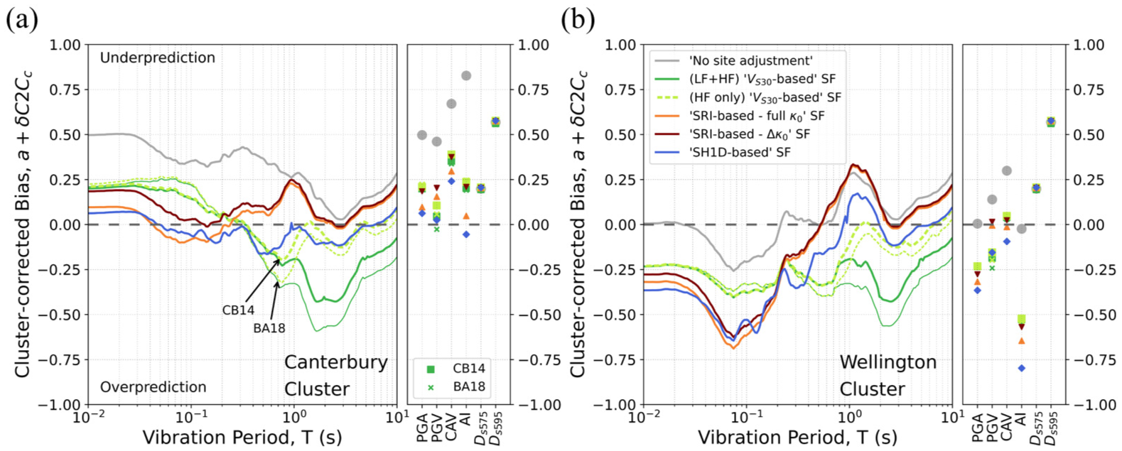
To further investigate the overall results in Figure 8, Figure 9 presents the model bias disaggregated by cluster (i.e. in terms of the systematic cluster residual, $a+\delta C2C_c$ ), revealing significant inter-cluster differences. Figure 9a shows that for the Canterbury cluster, the “SRI-based” and “SH1D-based” SFs reduce the underprediction exhibited by the “ $V_{S30}$ -based” SF method for PGA, CAV, AI, and $\mathrm{SA}(T<0.2s)$ , and overall, the “SH1D-based” SF method produces the lowest residuals for most of the IMs considered. The “SRI-based” SF methods produce underprediction in the period range associated with most of the $T_{\mathrm{SH}1D,0}$ values, suggesting that resonance effects are prominent in this cluster. In the case of the Wellington cluster, the “no site adjustment” simulation already exhibits a near-zero or negative bias for PGA, AI, and $\mathrm{SA}(T<0.6s)$ , and consequently, the site adjustments produce stronger overprediction for these and other IMs. The fact that this short-period overprediction is observed in the simulation before applying any site adjustment suggests that it corresponds to inaccuracies in the modeling of source and path effects for the Wellington cluster, as further illustrated in the following section. This shows the challenges involved in assessing the site adjustment performance based on the results of simulations, which involve source, path, and site components, as also alluded to by de la Torre et al. (2020).

Figure 9.

Cluster-corrected bias ( $a+\delta C2C_c$ ) for the (a) Canterbury and (b) Wellington clusters.

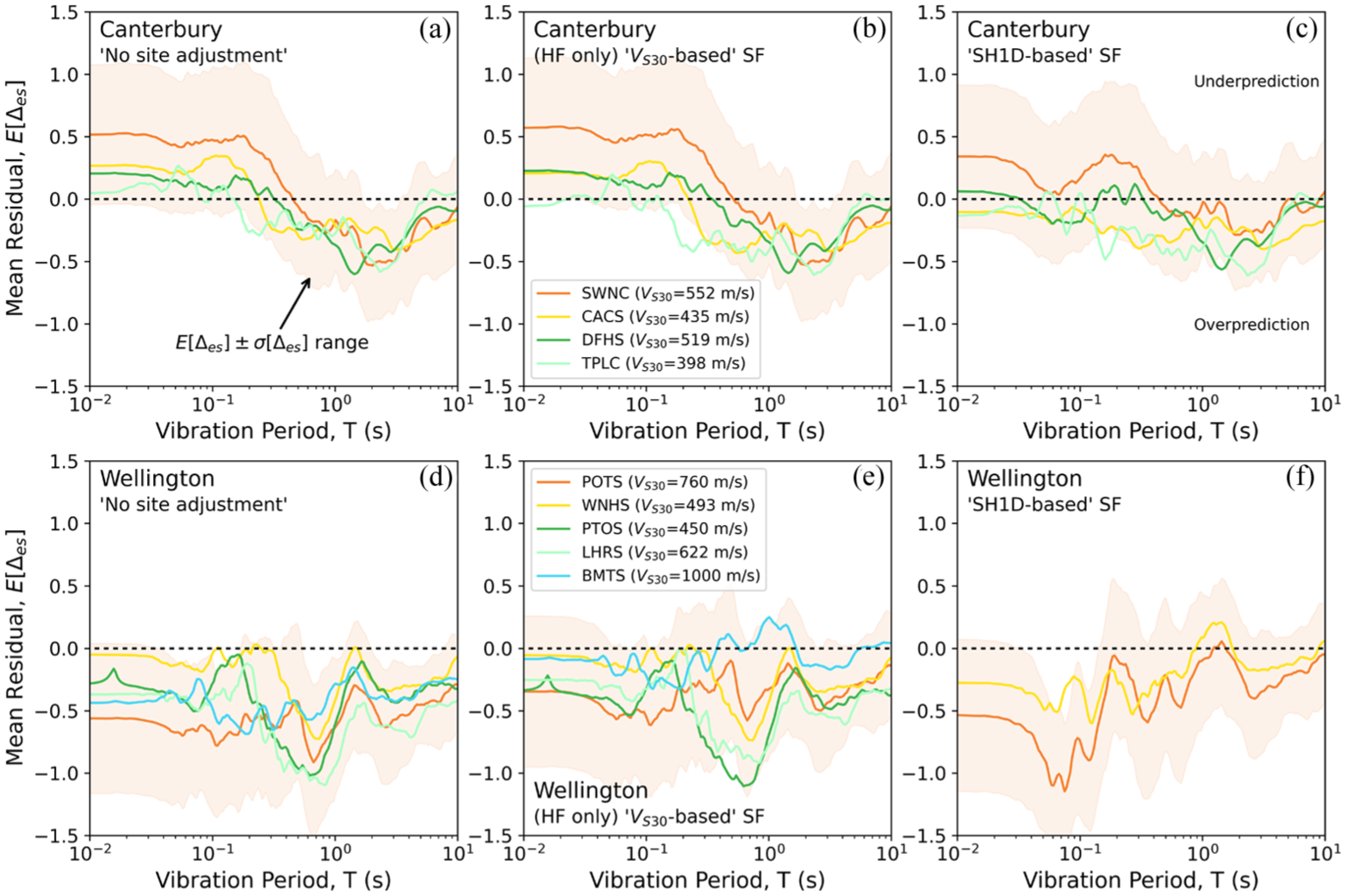
Prediction residuals at stiff soil and rock sites

Prediction residuals are first evaluated at stiff soil and rock sites to further investigate the accuracy of the regional ground-motion simulation and site-adjustment methods. For the Canterbury cluster, the four stiffest sites in the western side of Christchurch are considered (CACS, SWNC, DFHS, and TPLC), which are characterized by shallow gravels with $V_{S30}=398-552$ m/s. For the Wellington cluster, the stations POTS and WNHS located in Wellington City are used, which are classified as hill sites (de la Torre et al., 2024b; Nweke et al., 2022; Tiwari et al., 2023) and have $V_{S30}$ values of 760 m/s and 493 m/s, respectively. As explained in Electronic Supplement E, the $V_{S30}$ for POTS was inferred (based on de la Torre et al., 2024a; Kaiser et al., 2024) and its $V_S$ profile was estimated by modifying a $V_S$ measurement obtained near the station. Moreover, three additional rock sites located in Lower Hutt, not considered in the main validation study, have been included in this assessment to broaden the spatial coverage and obtain more robust inferences: PTOS, LHRS, and BMTS. These are hill sites without high-quality $V_S$ profiles available, but with inferred $V_{S30}$ values provided in Wotherspoon et al. (2024). The nine stiff soil and rock sites display a relatively flat site response as inferred from spectral decomposition using the generalized inversion technique (GIT) (Zhu et al., 2024), which suggests that strong site effects are absent.

Figure 10 presents the mean total residual, $E[{\mathrm{\Delta }}_{\mathrm{es}}]$ , for the “no site adjustment” simulation, and for the (HF only) “ $V_{S30}$ -based” (using the CB14 model) and “SH1D-based” SF methods (in the case of PTOS, LHRS, and BMTS the “SH1D-based” SF method is not considered). $E[{\mathrm{\Delta }}_{\mathrm{es}}]$ is used in this figure instead of systematic residuals because the PTOS, LHRS, and BMTS sites were not included in the mixed-effects regression. For the Canterbury sites, the “no site adjustment” simulation and the simulation adjusted by the (HF only) “ $V_{S30}$ -based” SF generally underpredict SA at short periods and overpredict it at long periods. The “SH1D-based” SF method reduces the bias, centering the residuals around zero. For the Wellington sites, the “no site adjustment” simulation generally overpredicts SA over the entire period range. The “ $V_{S30}$ -based” adjustment reduces this overprediction for the stiffest sites, but all the sites still maintain negative bias (overprediction) at short periods, which is also true for the “SH1D-based” SF method. This systematic overprediction at short periods for stiff soil and rock sites in Wellington provides additional evidence that the trend observed for the Wellington cluster in Figure 9b is likely caused by inaccuracies in the ground-motion simulation attributed to source and path effects. However, it should be noted that inaccuracies in the modeling of site effects (both in the simulation and in the posterior site adjustments) may also affect residuals for these stiff sites, and further investigation is needed to better understand the relative contributions of source, path, and site effects to the systematic residuals observed in Wellington.

Figure 10.

Mean residual for stiff and rock sites in Christchurch (a, b, and c) and Wellington (d, e, and f), for the “No site adjustment” simulation, the (HF only) “ $V_{S30}$ -based” SF method (using the CB14 model), and the “SH1D-based” SF method, respectively. The shaded area represents the ± one standard deviation range for the sites SWNC (top plots) and POTS (bottom plots).

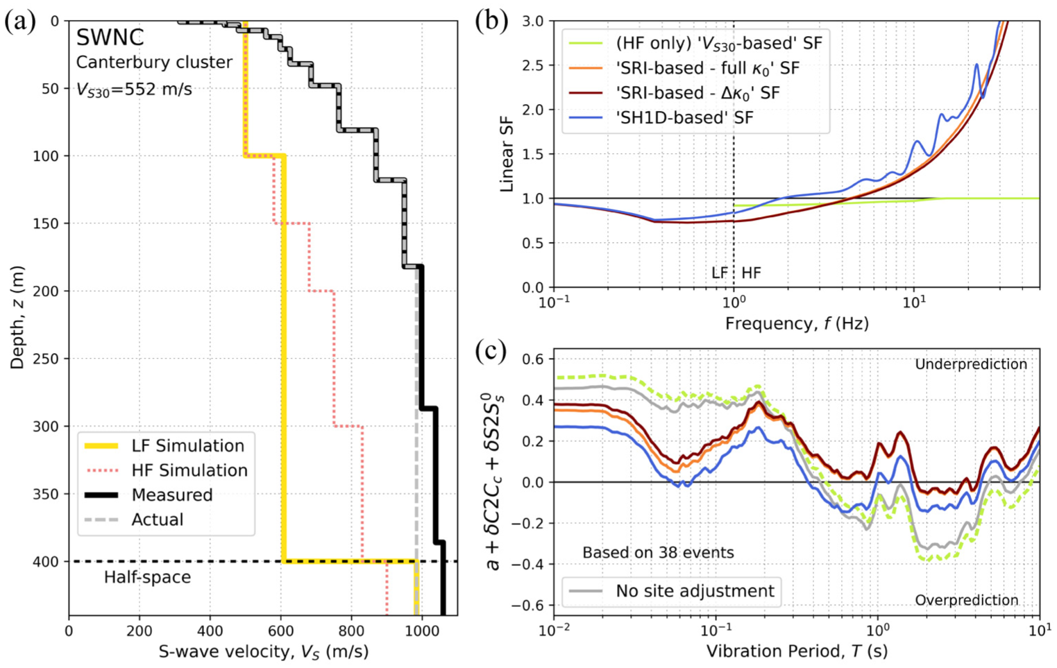
Figure 10c illustrated a case where the “SH1D-based” SF method improves prediction residuals for stiff sites relative to the (HF only) “ $V_{S30}$ -based” SF method. Figure 11 explains this residual reduction for the SWNC site. Figure 11a shows that the “measured” $V_S$ is significantly higher than the LF and HF “simulation” values in the top 400 m. An evaluation considering deep $V_S$ measurements at nine locations (Deschenes et al., 2018), presented in the Electronic Supplement E, reveals that this is a systematic trend in the western part of the Canterbury Plains. Figure 11b shows that the “SRI-based” and “SH1D-based” SFs are lower than unity at low frequencies and significantly higher at high frequencies. The deamplification at low frequencies results from correcting impedance effects (by using the “actual” profile, which is stiffer than the LF “simulation” profile) and brings the SA systematic residuals closer to zero at long periods (Figure 11c). The amplification at high frequencies results from adjusting attenuation effects. The stiffer “actual” profile produces less damping than the HF “simulation” profile, leading to the observed amplification in the computed site factors. This adjustment reduces the SA systematic residuals at short periods (Figure 11c). Hence, the “SRI-based” and “SH1D-based” adjustments improve the prediction for all vibration periods of interest. In contrast, the “ $V_{S30}$ -based” SF method is not able to capture these effects, and produces systematic residuals very similar to the regional simulation given that the $V_{S30}=552$ m/s of this site is close to the one considered in the simulation (500 m/s). A more rigorous treatment of the impedance effects discussed above should consider the explicit modification of the 3D velocity model in the western part of the Canterbury Plains, but the SFs derived here give an indication of the effect that this modification will have on the LF simulations.

Figure 11.

(a) $V_S$ profiles used to compute the $V_S$ profile-based SFs for the SWNC site, and comparison between (b) the linear SFs and (c) systematic residuals, for the different methods. The HF component of the $V_S$ profile-based SFs is presented with the HF normalization factor applied (i.e. $\mathrm{NF}·\mathrm{SF}$ ), although this factor has no observable effect at this site.

Comparison of site adjustments for soil sites

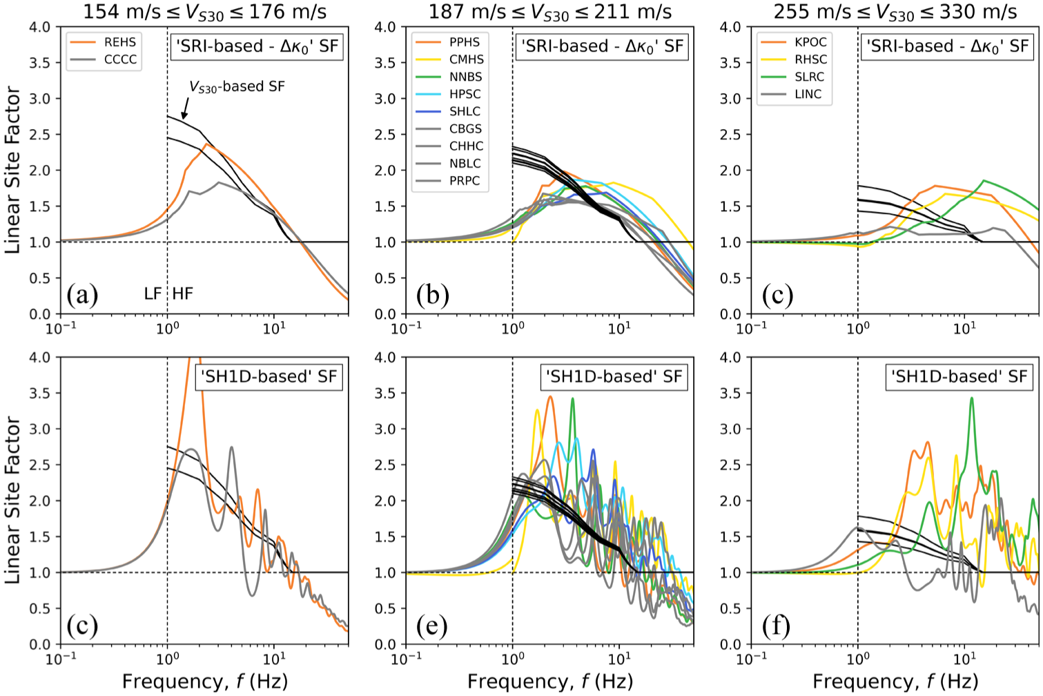
One question this article aims to answer is: do the $V_S$ profile-based methods (“SRI-based” or “SH1D-based” SFs) provide a significant improvement in ground-motion predictions at soil sites relative to the conventional “ $V_{S30}$ -based” SF method? To answer it, it is useful to first identify the situations where these SFs deviate more significantly from each other. The fact that soil nonlinearity is a second-order aspect in this study allows valuable insights to be obtained by simply comparing the linear components of the alternative SFs. Figure 12 displays the linear SFs computed with the alternative methods for 15 soil sites in Christchurch with $V_{S30}=154-330$ m/s. The sites have been grouped into three $V_{S30}$ bins, such that the within-bin variability of the “ $V_{S30}$ -based” linear SF is low. The (HF only) “ $V_{S30}$ -based” linear SF, computed with the CB14 model, is shown in the HF range only, to illustrate the approximate frequency range of influence. For the “SRI-based” approach, only the case with a $\Delta {\kappa }_0$ adjustment is considered, which allows for a more consistent comparison with the “SH1D-based” SF method. For the $V_S$ profile-based methods, the SFs are presented with the HF normalization factor applied. Figure 12 illustrates that the $V_S$ profile-based approaches, and particularly the “SH1D-based” SF method, result in significant within-bin variability, as opposed to the “ $V_{S30}$ -based” SF method. The sites where more significant differences are observed between the “ $V_{S30}$ -based” and “SH1D-based” SF methods have been heuristically selected and highlighted using different colors, whereas the rest of the cases are shown in gray.

Figure 12.

Comparison between the (HF only) “ $V_{S30}$ -based” linear SFs (computed with the CB14 model) and $V_S$ profile-based linear SFs, for soil sites in Christchurch grouped by different $V_{S30}$ bins. Narrow $V_{S30}$ ranges are considered such that the “ $V_{S30}$ -based” SFs are practically equivalent within a bin. a–c represent low, intermediate, and high $V_{S30}$ values, respectively, for the “SRI-based— $\Delta {\kappa }_0$ ” SF method; and d–f represent low, intermediate, and high $V_{S30}$ values, respectively, for the “SH1D-based” SF method. The HF component of the $V_S$ profile-based linear SFs is presented with the HF normalization factor applied (i.e. $\mathrm{NF}·\mathrm{SF}$ ). The peak of the “SH1D-based” SF for the REHS site reaches a peak of $\approx 4.5$ .

As shown in Figure 12, the maximum value of the (HF only) “ $V_{S30}$ -based” SF always occurs at $f=1$ Hz, with a decreasing trend at higher frequencies, up to f = 15 Hz, where it is truncated to unity. As discussed in Kuncar et al. (2025), the semi-empirical GMM used in the “ $V_{S30}$ -based” SF method implicitly accounts for deep 3D velocity structure effects, which in addition to host-to-target inconsistencies between the GMM and the ground-motion simulation properties, results in the high amplification at $f=1$ Hz. The maximum SF for the $V_S$ profile-based methods (i.e. “SRI-based— $\Delta {\kappa }_0$ ” and “SH1D-based” SF methods) occurs at $f>1$ Hz for these sites, with a considerable site-to-site variability. For all sites, the “SRI-based— $\Delta {\kappa }_0$ ” SF is significantly lower than its “ $V_{S30}$ -based” counterpart in the vicinity of $f=1$ Hz. This low amplification is explained by the the fact that the SRI-based adjustment is solely based on the shallow portion of the site (which, for these 15 sites, corresponds to the top 100 to 116 m), significantly influencing only $f>1$ Hz. The “SH1D-based” SF is also generally lower than the “ $V_{S30}$ -based” SF at 1 Hz, but higher than the “SRI-based— $\Delta {\kappa }_0$ ” SF, due to the consideration of resonance effects. When the near-surface predominant frequency, $f_{\mathrm{SH}1D,0}$ , is close to $f=1$ Hz, a significant level of amplification is generally exhibited at $f=1$ Hz by the “SH1D-based” SF. For the six sites identified as displaying less differences between the “SH1D-based” and “ $V_{S30}$ -based” SFs (CCCC, CBGS, CHHC, NBLC, PRPC, and LINC), $f_{\mathrm{SH}1D,0}$ is in the range $1-2$ Hz. As observed in Figure 12d for CCCC, in most of these sites the “SH1D-based” SF oscillates around the “ $V_{S30}$ -based” SF, with a similar average amplification in the range $f=1-15$ Hz.

Cases identified as displaying significant differences between the “SH1D-based” and “ $V_{S30}$ -based” linear SFs are those where (1) for relatively soft sites, there is large resonance-based amplification in the “SH1D-based” SF over narrow frequency bands (e.g. REHS and PPHS), and (2) for relatively stiff sites, significant amplification occurs at frequencies considerably higher than 1 Hz, where the “ $V_{S30}$ -based” SF is low (e.g. sites KPOC, RHSC, and SLRC). As shown in Figure 12f, the relatively high $V_{S30}$ of these sites results in low $V_{S30}$ -based amplification and low attenuation in the “SH1D-based” SF, accentuating the differences at high frequencies. This generates frequency bands with very large differences between the two methods. For example, for SLRC, the $V_{S30}$ -based amplification at $f\approx$ 12 Hz is close to 1, whereas the SH1D-based prediction is 3.4. Figure 12c shows that the “SRI-based— $\Delta {\kappa }_0$ ” SF also predicts higher levels of high-frequency amplification than the $V_{S30}$ -based approach for these sites.

Supplemental Figure E.4 in Electronic Supplement E shows equivalent results for 13 soil sites in the Wellington cluster with $V_{S30}=223-375$ m/s, and illustrates another situation where large differences can occur between methods: sites with $f_{\mathrm{SH}1D,0}$ considerably lower than the transition frequency of 1 Hz (e.g. TFSS), where a significant amplification is predicted near $f_{\mathrm{SH}1D,0}$ by the “SH1D-based” SF method and no amplification is considered by the (HF only) “ $V_{S30}$ -based” SF method.

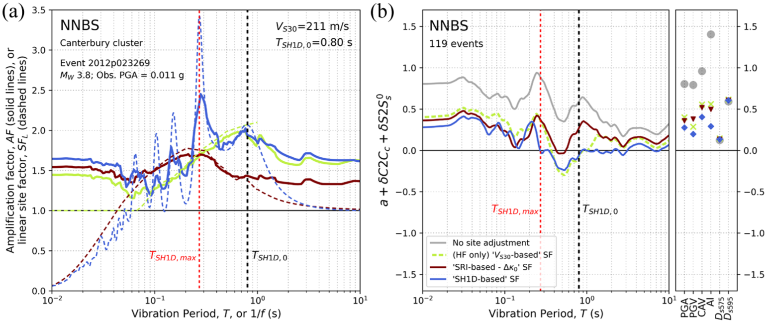
Once the sites with more (and less) differences between the $V_S$ -based and $V_{S30}$ -based SFs are identified, the following question is: what is the effect of these differences on the prediction residuals? Figure 13 illustrates this effect for the NNBS site, identified in Figure 12b as presenting significant between-method differences. Figure 13a first shows the effect of the SF (which is applied in the Fourier spectral domain) on the SA amplification factor, AF (which is computed in the response spectral domain as AF = $S{A}_{\mathrm{adj}}$ / $S{A}_{\mathrm{sim}}$ ; where $S{A}_{\mathrm{adj}}$ is the adjusted SA for a given method and $S{A}_{\mathrm{sim}}$ is the SA for the “no site adjustment” simulation). The linear SFs (plotted with dashed lines) are presented as a function of 1/f, to superimpose them with the AFs (plotted with solid lines) computed for one particular event. The overall shapes of the linear SFs and the corresponding AFs are similar in the period range $T=0.09-0.8$ s, but in the case of the “SH1D-based” SF method the amplitude of the peaks is lower (and the amplitude of the troughs is higher) for the AF than for the SF. For example, the maximum resonant peak at this site (illustrated in the figure at $T=T_{\mathrm{SH}1D,\max }$ ), presents a reduction of ≈ 30% in its amplitude, from the linear SF to the AF. This smoothing of the resonant peaks and troughs implies that large differences in the SFs between the “SH1D-based” and “ $V_{S30}$ -based” SF methods are reduced when comparing the SA prediction residuals. This is illustrated in Figure 13b, where it is shown that the SA systematic residual for the “ $V_{S30}$ -based” and “SH1D-based” SF methods are relatively similar over the entire period range, with a more considerable difference at $T_{\mathrm{SH}1D,\max }$ (consistent with the AF difference observed in Figure 13a for one event), where the “SH1D-based” SF method improves predictions. At very short ( $T<0.09$ s) and long ( $T>1.0$ s) vibration periods, the SFs departs considerably from corresponding AFs (for all methods), which is explained by the fact that response spectra at these periods are dominated by a wide range of (signal) frequencies for small-magnitude events (Stafford et al., 2017). As a result, the significant differences observed in Figure 13a between the SFs for the SH1D- and $V_{S30}$ -based approaches, particularly at short periods, do not manifest as a significant difference in the corresponding AFs and systematic residuals (Figure 13b).

Figure 13.

Illustration of the effect of different site factors on systematic residuals for different IMs, for the NNBS site. (a) Comparison between the amplification factors (AFs) for an individual event, plotted with solid lines, and linear site factors ( $S{F}_L$ s), shown with dashed lines, for different methods; and (b) comparison of systematic residuals for different methods and IMs.

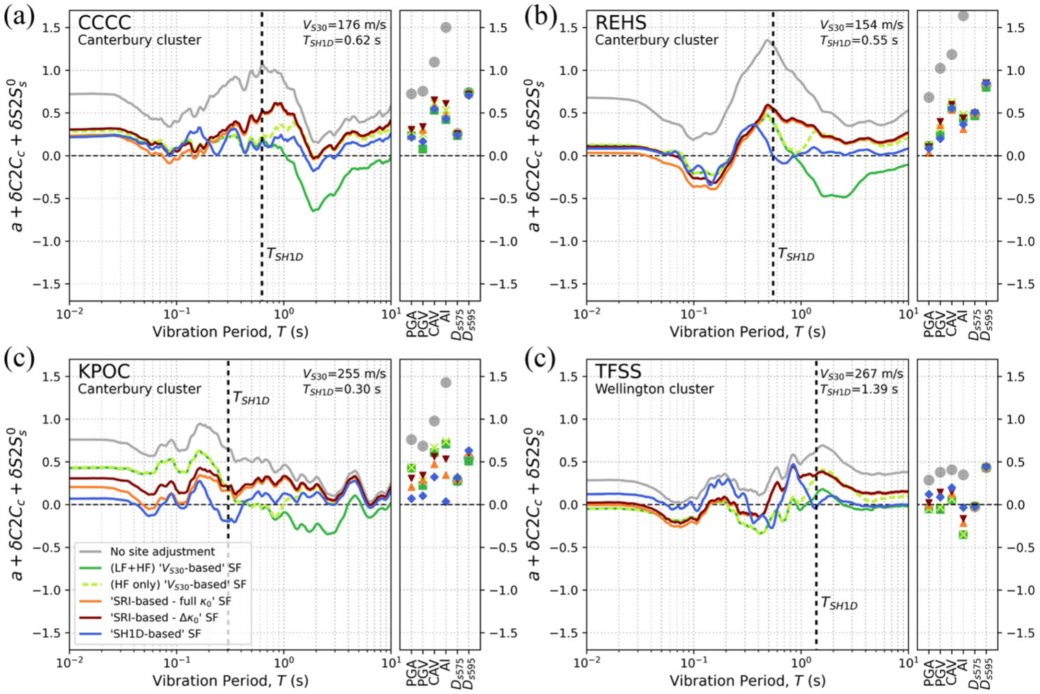
Figure 14 presents the systematic residuals for four additional sites (the systematic residuals for all sites considered are provided in Electronic Supplement D). CCCC (Figure 14a) is an example of a site in Canterbury, identified in Figure 12 as not displaying significant differences between the (HF only) “ $V_{S30}$ -based” and the “SH1D-based” linear SFs, and Figure 14a shows that this results in very similar residuals between these two methods for all IMs. REHS (Figure 14b) and KPOC (Figure 14c) are examples of sites in Canterbury, identified in Figure 12, as exhibiting significant differences between the “ $V_{S30}$ -based” and “SH1D-based” SFs. For REHS, this difference is due to a strong resonant peak at $f_{\mathrm{SH}1D,0}$ . As observed in Figure 14b, this results in a significant improvement in the SA systematic residuals at $T_{\mathrm{SH}1D,0}$ for the “SH1D-based” SF relative to the other methods, which underpredict SA (further evidence of the improvement in prediction obtained by using the “SH1D-based” approach at REHS is provided in Supplemental Figure E.5 in Electronic Supplement E). Similar improvement at $T_{\mathrm{SH}1D,0}$ is observed for the HPSC site, which was also identified as displaying a relatively strong resonant peak at $f_{\mathrm{SH}1D,0}$ in the “SH1D-based” SF. For KPOC, strong resonant peaks at relatively high frequencies are observed in Figure 12f, and this results in a significant reduction of the systematic residuals for PGA, PGV, CAV, AI, and SA at short vibration periods for the “SH1D-based” SF method relative to the “ $V_{S30}$ -based” approach. The “SRI-based” SFs also improve predictions at short vibration periods, but to a lesser extent. Similar improvements in the residuals are consistently observed for the RHSC and SLRC sites, which also present high-frequency resonant peaks (Figure 12f). Finally, TFSS (Figure 14d) was identified in Supplemental Figure E.4 as exhibiting significant differences between the (HF only) “ $V_{S30}$ -based” and “SH1D-based” SFs due to a strong resonant peak occurring at $f_{\mathrm{SH}1D,0}$ , which is considerably lower than 1 Hz. Similar to the NNBS and REHS sites, this situation produces a local reduction in the systematic residual at $T_{\mathrm{SH}1D,0}$ for the “SH1D-based” SF method. For all four sites, Figure 14 also includes the results for the (LF + HF) “ $V_{S30}$ -based” SF method. In the case of the CCCC, REHS, and KPOC sites, the consideration of the LF site factor results in a considerable overprediction at long vibration periods, but for TFSS this implementation provides lower residuals than the (HF only) “ $V_{S30}$ -based” SF method, which underestimates SA. Since for this site $f_{\mathrm{SH}1D,0}<1$ Hz, the application of the SF to the LF component partially captures the increase in amplification in the LF range due to the resonant peak. For the NNBS (Figure 13b), CCCC, REHS, and TFSS (Figure 14) sites, the “SRI-based” SF methods result in considerable underprediction at $T_{\mathrm{SH}1D,0}$ , and the “SH1D-based” SF method significantly improves SA prediction at this period, suggesting the presence of resonance effects.

Figure 14.

Systematic residuals for the different methods, for the sites (a) CCCC, (b) REHS, (c) KPOC, and (d) TFSS.

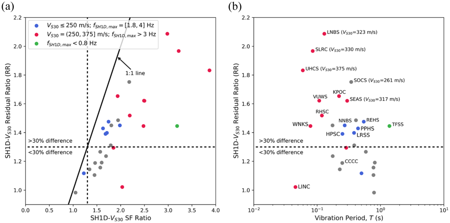
Figure 15 summarizes the differences between the “ $V_{S30}$ -based” and “SH1D-based” methods considering all soil sites in Christchurch and Wellington with $V_{S30}\le 375$ m/s. The maximum amplitude in the linear “SH1D-based” SF between 0.1 and 25 Hz was first extracted, and the frequency at which it occurs ( $f_{\mathrm{SH}1D,\max }$ ) was obtained. Then, the linear “ $V_{S30}$ -based” SF was evaluated at $f_{\mathrm{SH}1D,\max }$ , and the ratio between the linear “SH1D-based” SF ( $S{F}_{\mathrm{SH}1D}$ ) and linear “ $V_{S30}$ -based” SF ( $S{F}_{V_{S30}}$ ) amplitudes was computed as

$$\mathrm{SH}1\mathrm{D}-V_{S30}\mathrm{SF}\mathrm{ratio}=\frac{S{F}_{\mathrm{SH}1D}\left(f_{\mathrm{SH}1D,\max }\right)}{S{F}_{V_{S30}}\left(f_{\mathrm{SH}1D,\max }\right)}$$

(8)

The “SH1D- $V_{S30}$ SF ratios” are plotted on the x-axis of Figure 15a. Similarly, the ratio between the exponential of the SA systematic residuals for these two methods was evaluated at $T=1/f_{\mathrm{SH}1D,\max }$ (in this case the “ $V_{S30}$ -based” SF method is considered in the numerator to get a comparable ratio). This ratio (“SH1D- $V_{S30}$ residual ratio”) is plotted on the y-axis of Figure 15a. As observed, the residual ratios (RRs) are systematically lower than the SF ratios, as a result of the smoothing produced in the response spectral domain. For example, Figure 15a shows that SF ratios $>1.3$ are obtained for 93% of the sites, whereas for the residual ratios this is only true for 59% of them.

Figure 15.

Difference between the “ $V_{S30}$ -based” and “SH1D-based” SF methods at $f_{\mathrm{SH}1D,\max }$ for all soil sites considered with $V_{S30}\le 375$ m/s. (a) Residual ratios (RR) vs SF ratios; (b) Residual ratios (RR) vs vibration period, T, where $T=T_{\mathrm{SH}1D,\max }$ .

Figure 15b presents the RRs as a function of vibration period, and illustrates that the highest RRs tend to occur for relatively short vibration periods. Three groups of sites are identified: (1) sites with $V_{S30}\le 250$ m/s and $f_{\mathrm{SH}1D,\max }=1.8-4$ Hz; (2) sites with $V_{S30}=250-375$ m/s and $f_{\mathrm{SH}1D,\max }>3$ Hz; and (3) sites with $f_{\mathrm{SH}1D,\max }<0.8$ Hz. These cases cover most of the situations where significant RRs ( $\mathrm{RR}>1.3$ ) are obtained, and Figure 15b illustrates that case (2) generally results in the highest departure between systematic residuals of the two methods. Figures 13 and 14 illustrated that in cases with high RRs, the “SH1D-based” SF method often produces a reduction in the systematic residuals. Since the Wellington cluster displays systematic overprediction at short vibration periods, likely related to source and path effects as previously discussed, an evaluation of this type is more challenging. GIT full site responses (Zhu et al., 2024) confirm that some of these sites (e.g. SOCS, LRSS, SEAS, WNKS) display observable resonances in the vicinity of $f_{\mathrm{SH}1D,\max }$ (and/or $f_{\mathrm{SH}1D,0}$ ), which suggests that in these cases the “SH1D-based” SF method should improve predictions if the simulation of source and path effects were unbiased. Supplemental Figure B.41 in Electronic Supplement B illustrates that in several cases, mHVSR identifies peaks around $f_{\mathrm{SH}1D,\max }$ , where significant RRs are found at relatively high frequencies (e.g. UHCS, LNBS and SOCS sites in Wellington; SLRC, NNBS, and KPOC sites in Canterbury). This suggests that mHVSR measurements could help inform site-response method selection (particularly, at sites where a $V_S$ profile is not yet available).

Site response relative to a reference site

An alternative to further isolate site response from path and source effects, in the evaluation of the alternative SF methods, is to compare the observed and simulated site amplification at a given target soil site with respect to a nearby “reference” station characterized by low site response. This approach is particularly valuable in the case of Wellington, where inferences on SF method validity through residual analysis was shown to be challenging due to the systematic overprediction of the ground-motion simulations at short vibration periods. Ideally, the selection of the reference and target sites should be such that differences in the observed SA mainly reflect local site effects at the target site (Borcherdt, 1970; Ntritsos et al., 2021). However, even rock reference stations may be affected by some level of site response (e.g. Steidl et al., 1996). In the following analysis, the same SF method used to modify the simulated ground motion at the target site is consistently used for modifying the corresponding ground motion at the reference site. In this way, the question to be answered is: which method better models the relative site response between the target and reference sites?

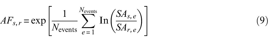
The target sites considered are three stations located in the Thorndon basin (WEMS, TFSS, and VUWS) and two stations located in the Te Aro basin (FKPS and TEPS), in Wellington City (see Figure 1). Observations and numerical modeling (e.g. Bradley et al., 2017, 2018; McGann et al., 2021) have suggested the occurrence of basin-edge effects (Kawase, 1996) in the Thorndon basin, due to the Wellington Fault creating a steep-sided boundary (as illustrated in Figure 3c). The station POTS is used as the reference site, similar to several previous studies in the same region (e.g. Bradley et al., 2017, 2018; de la Torre et al., 2024a; Kaiser et al., 2024; Lee et al., 2024; McGann et al., 2021). The relatively short distances between the five target sites and POTS with respect to the large source-to-site distances (Figure 1), minimizes the influence of source and path effects in the site-response ratios, which is optimal for the evaluation of site effects (Borcherdt, 1970; Ntritsos et al., 2021). As explained in Electronic Supplement E, the actual $V_S$ profile considered for POTS is based on a measured $V_S$ profile close to this station, modified to have a $V_{S30}=760$ m/s, considered representative for POTS (e.g. de la Torre et al., 2024a; Kaiser et al., 2024). The relative site amplification between the target and reference sites, $A{F}_{s,r}$ , is computed using the following expression:

$$A{F}_{s,r}=\exp \left[\frac{1}{N_{\mathrm{events}}}\sum _{e=1}^{N_{\mathrm{events}}}\mathrm{In}\left(\frac{S{A}_{s,e}}{S{A}_{r,e}}\right)\right]$$

(9)

where $S{A}_{s,e}$ is the observed or simulated SA at the target site s for the event e; $S{A}_{r,e}$ is the corresponding SA at the reference site r (POTS in this case); and $N_{\mathrm{events}}$ is the number of events simultaneously recorded at the target site and reference site.

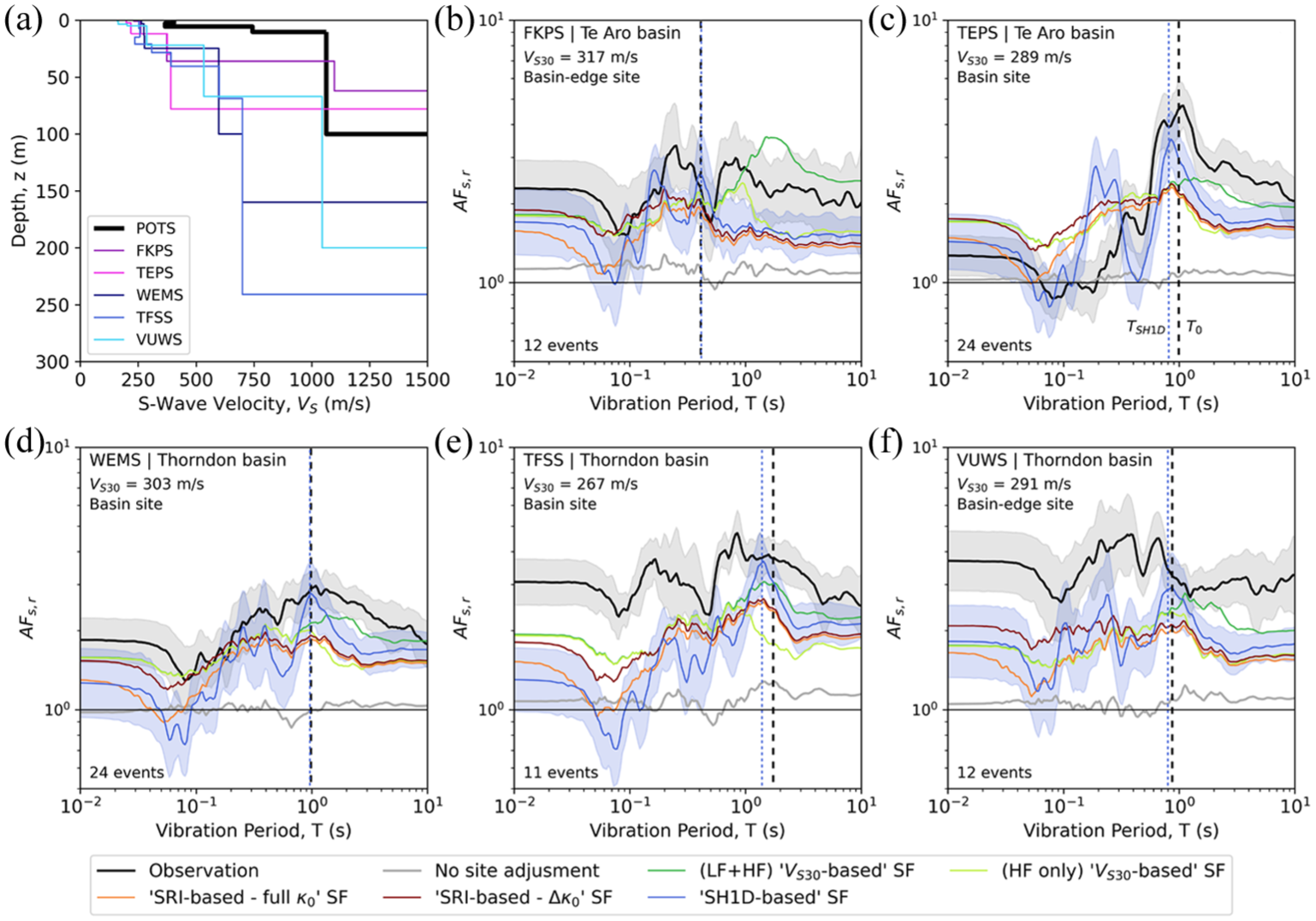
Figure 16 shows the results of this analysis for the observed and simulated ground motions modified by the different SF methods considered. The SA ratios for the “no site adjustment” case is close to unity for all sites and vibration periods. This indicates that the simulation is not able to capture 3D site effects. In the case of the LF simulation component, this is mainly due to the grid spacing (100 m) and minimum $V_S$ (500 m/s) considered, which do not allow for properly modeling the basin geometry of this shallow basin (Supplemental Figure E.6 in Electronic Supplement E shows an example of this). In the case of the HF simulation component, it is due to the use of a generic 1D $V_S$ profile.

Figure 16.

(a) $V_S$ profiles, and comparison of observation and predictions of site response relative to the reference station POTS, for the sites (b) FKPS, (c) TEPS, (d) WEMS, (e) TFSS, and (f) VUWS. Shaded areas in gray and blue represent the ± one standard deviation range for the “Observation” and “SH1D-based” SF, respectively. The indicated “basin” and “basin-edge” site classifications follow the scheme of Nweke et al. (2022); Tiwari et al. (2023).

Figure 16 shows that $T_{\mathrm{SH}1D,0}$ and $T_0$ (provided by Wotherspoon et al., 2024) are similar for the five sites, illustrating that the “SH1D-based” SF captures the estimated fundamental site periods relatively well. Furthermore, the “SH1D-based” SF tends to better capture the observed site amplification at $T_{\mathrm{SH}1D,0}$ than the other methods, which generally underpredict it. For example, Figure 16c (TEPS site) shows that all the other methods underpredict the site amplification at $T_{\mathrm{SH}1D,0}$ by $\approx 40$ %, while the “SH1D-based” prediction is only $\approx 15$ % lower than the observation. Figure 16e (TFSS site) illustrates a significant difference between the “SH1D-based” and (HF only) “ $V_{S30}$ -based” SF methods at $T_{\mathrm{SH}1D,0}$ (which is greater than 1 s). In this case, the “SH1D-based” prediction is only ≈ 5% lower than the observation, whereas for the (HF only) “ $V_{S30}$ -based” approach the underprediction increases to $\approx 50$ %. Even though the “SH1D-based” SF method provides better predictions than the other methods at $T_{\mathrm{SH}1D,0}$ , the same is not necessarily true at other vibration periods. In the case of TEPS, the observed peak occurs within a narrow period range, which resembles the “SH1D-based” prediction, resulting in relatively good performance of the “SH1D-based” SF method in the vicinity of $T_{\mathrm{SH}1D,0}$ . In contrast, for the sites in the Thorndon basin the observed “peak” site response occur over a much broader period range, which result in significant underprediction for the “SH1D-based” SF method at periods around $T_{\mathrm{SH}1D,0}$ . At $T<T_{\mathrm{SH}1D,0}$ , the SH1D-based prediction produces some peaks and troughs that significantly overpredict or underpredict the response over narrow period ranges. This behavior is influenced by the significant uncertainty in the (modified) $V_S$ profile used for POTS. At $T>1$ s, the (LF + HF) “ $V_{S30}$ -based” SF method results in the best predictions for TEPS, WEMS, TFSS, and VUWS (for FKPS, the shallowest site, this method generates overprediction), compensating for unmodeled 3D effects in the LF simulation.

The TFSS and VUWS sites exhibit significant underprediction at short vibration periods across all site-adjustment methods. This underprediction is substantially greater than the differences observed between methods, suggesting that a large portion of the underprediction is due to the inability of the regional simulation to capture 3D effects at short vibration periods.

Conclusion

This paper presented a comprehensive validation of four methods to account for shallow site effects in hybrid broadband ground-motion simulation, using 213 small-magnitude earthquakes recorded at 38 well-characterized strong-motion station sites in New Zealand. The site-adjustment methods considered are based on either $V_{S30}$ or a $V_S$ profile (including SRI-based and SH1D-based approaches), and their relative performance was primarily assessed through residual analysis of different intensity measures (IMs) of engineering interest. A question this study aimed to answer was: can using more comprehensive site-characterization data (i.e. a $V_S$ profile instead of a $V_{S30}$ value) significantly improve predictions?

The incorporation of shallow site effects with any of the methods considered significantly reduced the prediction site-to-site variability for PGA, PGV, CAV, AI, and pseudo-spectral acceleration (SA) over a wide range of vibration periods; but overall, this reduction was comparable for the different methods. The Wellington cluster exhibited a systematic overprediction for SA at short vibration periods, which is likely related to inaccuracies in the simulation of source and path effects. For the Canterbury cluster, the use of any of the methods considered significantly reduced the underprediction of the regional simulations, with the $V_S$ profile-based methods further reducing the model bias for PGA, CAV, AI, and SA at short vibration periods, relative to the $V_{S30}$ -based approach.

The SRI-based methods generally resulted in SA underprediction for soil sites at the predominant frequency of the near-surface profile ( $f_{\mathrm{SH}1D,0}$ ), suggesting that shallow resonance effects are prominent in the studied regions. Four situations were identified where significant differences are observed between the (HF only) $V_{S30}$ - and SH1D-based methods, and the latter tends to improve predictions: (1) stiff sites for which simulations overestimate attenuation effects (e.g. SWNC, DFHS); (2) relatively stiff sites ( $V_{S30}$ = 250–375 m/s) with high-frequency ( $f_{\mathrm{SH}1D,0}>3$ Hz) resonances (e.g. KPOC, RHSC, SLRC, UHCS); (3) relatively soft sites ( $V_{S30}\le 250$ m/s) with very strong resonances in the 1.8–4.0 Hz frequency range (e.g. NNBS, PPHS, REHS, HPSC), and (4) sites with $f_{\mathrm{SH}1D,0}<0.8$ Hz (e.g. TFSS).

This study showed that the proper incorporation of shallow site effects can greatly improve the predictive capabilities of hybrid broadband ground-motion simulation for several IMs. At the same time, it demonstrated that using more advanced approaches based on the SRI method or the SH1D transfer function does not necessarily result in further improvements in overall simulation precision. Parametric and modeling uncertainties involved in physics-based site-response approaches that rely on a 1D site representation (i.e. SRI method and SH1D transfer function), in addition to uncertainties and limitations of the regional ground-motion simulations, resulted in overall comparable performance with the simpler empirical $V_{S30}$ -based adjustment. Furthermore, this study showed that the smoothing of the Fourier-based site amplification produced in the response spectral domain also contributed to reducing the differences between the considered methods. Particular situations identified as leading to significant differences between the $V_{S30}$ -based approach and more sophisticated methods can be considered when selecting site-adjustment methods in forward applications.

This paper highlighted the importance of properly assessing source and path modeling in the regional simulation when judging the prediction capabilities of different site-adjustment methods. Further research is needed to better understand the relative contribution of source, path, and site effects on the residuals, which will necessarily require the incorporation of additional observational data. A key step to broaden the applicability of this study is to evaluate the performance of different site-adjustment methods (including time-domain approaches) for higher-amplitude ground motions that induce more significant levels of soil nonlinearity.

Supplemental Material

sj-pdf-1-eqs-10.1177_87552930251377784 – Supplemental material for Validating alternative methods to account for shallow site effects in hybrid broadband ground-motion simulation of small-magnitude earthquakes in New Zealand

Supplemental material, sj-pdf-1-eqs-10.1177_87552930251377784 for Validating alternative methods to account for shallow site effects in hybrid broadband ground-motion simulation of small-magnitude earthquakes in New Zealand by Felipe Kuncar, Brendon A Bradley, Christopher A de la Torre, Adrian Rodriguez-Marek, Chuanbin Zhu and Robin L Lee in Earthquake Spectra