
Abstract
Shallow site effects are indirectly considered in conventional hybrid broadband ground-motion simulations, and their proper incorporation may be key to improving ground-motion predictions at soil sites. This article presents and examines five methods to adjust hybrid simulations to account for these effects. These methods use different approaches to modeling site response and require different amounts of site-characterization data: Methods 1 and 2 use only proxy parameters (e.g.
Keywords
Introduction
Physics-based ground-motion simulations require the modeling of source, path, and site effects. The latter refer to the influence that the local geology and geomorphology of the site have on ground shaking (Stewart et al., 2017) and include seismic wave reflection and refraction, impedance-based amplification, anelastic attenuation, and soil nonlinearity. These phenomena can significantly modify the amplitude, frequency content, and duration of the ground motion (Kramer, 1996), and hence, their proper modeling may be key to improve physics-based ground-motion predictions at soil sites, as suggested by recent validation studies (e.g. de la Torre et al., 2020; Lee et al., 2020, 2022). Whereas 3D regional-scale simulations are usually performed adopting a domain length of tens or hundreds of kilometers, which is needed to capture source and path effects, near-surface site effects occur on a scale of meters and require a finer spatial resolution in regional-scale modeling than that typically considered. Two reasons hinder the explicit incorporation of these near-surface materials in 3D regional-scale simulations: (1) the high computational cost required and (2) the lack of detailed knowledge of the near-surface material properties at the specific site of interest and in the surrounding area. These two factors are particularly important when soil nonlinearity is significant, which is typically the case for design-level ground motions.
As a result, most studies that have explicitly modeled near-surface materials in 3D regional-scale simulations, including soil nonlinearity (e.g. Dupros et al., 2010; Fu et al., 2017; Paolucci et al., 2016; Seylabi et al., 2021; Smerzini et al., 2017; Taborda et al., 2012), considered one or more simplifications: for example, (1) an idealized characterization of the sedimentary basin, represented by thick and homogeneous layers (e.g. Dupros et al., 2010; Taborda et al., 2012); or (2) a simplified modeling of soil nonlinearity, either using elastic-perfectly plastic constitutive models (e.g. Dupros et al., 2010; Fu et al., 2017; Taborda et al., 2012) or a simplified nonlinear viscoelastic approach (e.g. Paolucci et al., 2016; Smerzini et al., 2017). As an alternative, other studies have adopted an “uncoupled approach,” where the regional-scale simulation is produced without explicitly incorporating the near-surface soil materials, and the resulting ground-motion time series is adjusted to account for unmodeled local site effects. The adjustment has been performed in the frequency domain (e.g. Graves and Pitarka, 2010; Lee et al., 2022; Pilz et al., 2021; Razafindrakoto et al., 2021; Rodgers et al., 2020; Shi, 2019) and in the time domain (e.g. de la Torre et al., 2020; Evangelista et al., 2017; Hartzell, 2002; Roten et al., 2012). This modular approach does not require a significant increase in the computational effort and can make use of more localized site-characterization data. It also has all the practical benefits of making the two processes (regional-scale simulation and site effects modeling) independent, such as allowing the site-response modeling to be done at any time after the regional-scale simulation is performed (e.g. when the location-specific site-characterization data become available), or allowing different groups of professionals (i.e. engineering seismologists vs geotechnical earthquake engineers) to deal with the two parts of the problem. However, an important limitation of this approach is that 3D site effects can be overlooked (e.g. Seylabi et al., 2021) depending on the specific implementation adopted.
Regarding the ground-motion simulation methodology, hybrid methods (e.g. Graves and Pitarka, 2010; Hartzell et al., 1999; Mai et al., 2010; Ojeda et al., 2021; Paolucci et al., 2021) are currently the most widely used in engineering applications, due to their ability to generate realistic broadband ground-motion time series in the frequency range of interest for structural and geotechnical systems (Baker et al., 2021). In this approach, the low-frequency (LF) and high-frequency (HF) components of the ground motion are simulated using different methods. The most common way in which local site effects have been considered in this methodology is through the uncoupled approach, and particularly, through a frequency-domain adjustment using site-correction factors derived from semi-empirical ground-motion models (GMMs) (e.g. Graves and Pitarka, 2010; Lee et al., 2022; Razafindrakoto et al., 2021). In this method, usually only the 30 m time-average shear-wave velocity,
Although modeling of local site effects has been widely investigated in the literature as an individual component (e.g. Hallal and Cox, 2021; Kaklamanos et al., 2013), or as part of site-specific adjustments to seismic hazard analysis (e.g. NRC, 2021; Rodriguez-Marek et al., 2021; Stewart et al., 2017), relatively little attention has been given to its treatment in the context of hybrid broadband ground-motion simulations. This simulation methodology imposes specific considerations that require further examination. Specifically, questions that need to be addressed are: (1) what are the key elements for compatibility between the regional-scale simulation and subsequent site-response adjustment, and hence the theoretical attributes that the different methods to perform this adjustment should consider? (2) What are the limitations of the commonly used
This study presents a comprehensive examination of the aforementioned issues. First, the different approaches that can be used to model local site effects are examined. Second, the main aspects that must be considered to properly adjust hybrid broadband ground-motion simulations are discussed. Next, a case study is described, which is then used to discuss five methods for performing the site-response adjustment and compare the resulting site amplification factors (AFs). These methods can be applied in the presence of different levels of site-characterization data. In particular, Method 1 is the conventional
Approaches for modeling local site effects
Overview
Figure 1a presents five general approaches (Approaches A–E) that can be used to model site effects in a broad range of applications (e.g. empirical or physics-based ground-motion modeling), and Figure 1b illustrates their relationship with the five methods (Methods 1–5) examined in this article, which are specifically tailored to adjusting hybrid broadband ground-motion simulations. Approaches A–E are discussed below, while the site-adjustment Methods 1–5 are described in the “Methods for performing site adjustments to hybrid broadband ground-motion simulation” section.
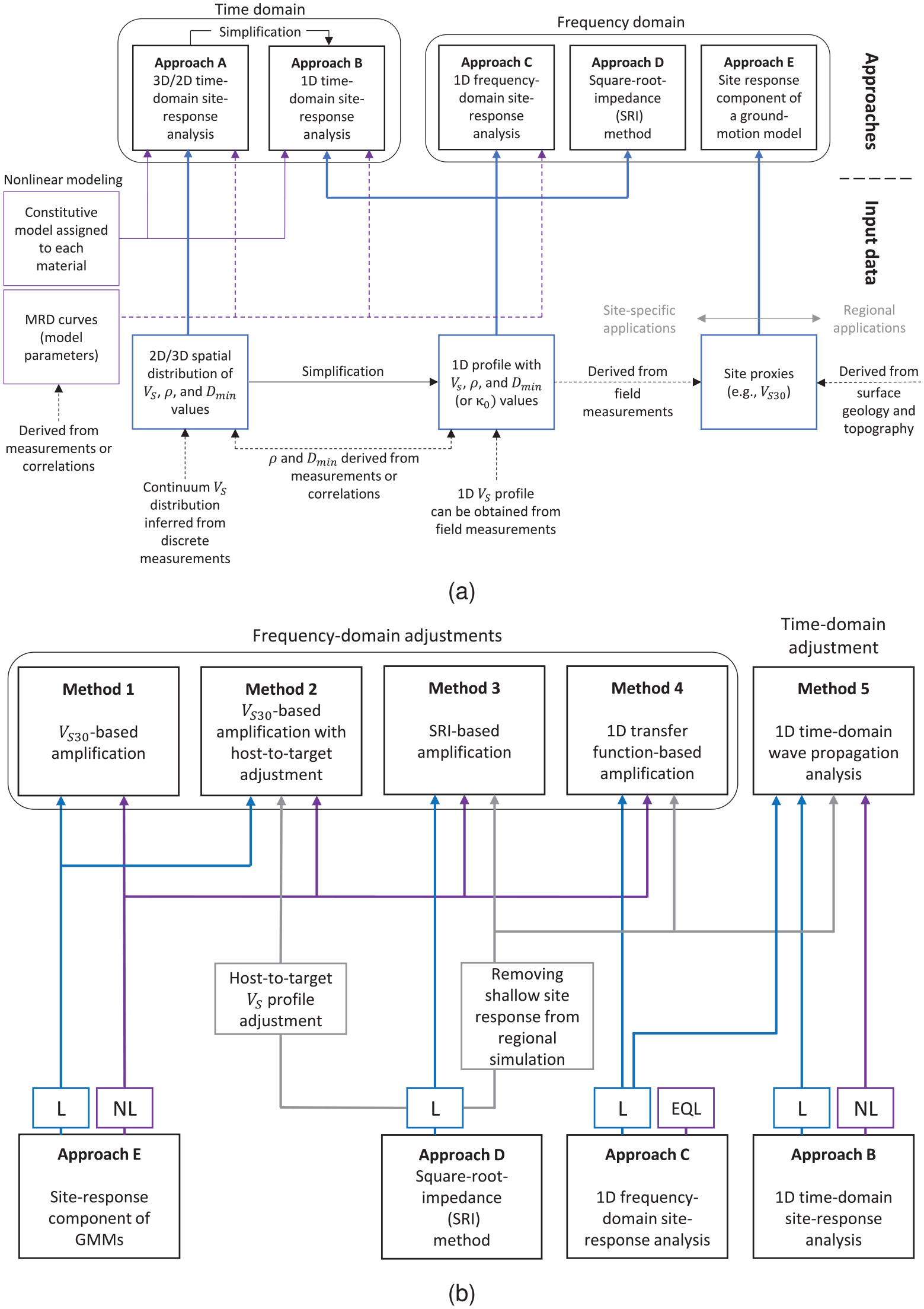
(a) Time-domain and frequency-domain approaches to model site effects, and their respective input data. (b) The relationship between these approaches and the investigated methods to perform site adjustments to hybrid broadband ground-motion simulations. L: linear; NL: nonlinear; EQL: equivalent-linear.
As illustrated in Figure 1a, going from Approach A to E implies the use of incrementally less site information and the introduction of some simplifications in the description of the site conditions and wave-propagation phenomena. Table 1 provides a comparison between these five approaches in terms of their relative advantages and disadvantages, and further discussion is provided below.
Comparison of different approaches to model site effects
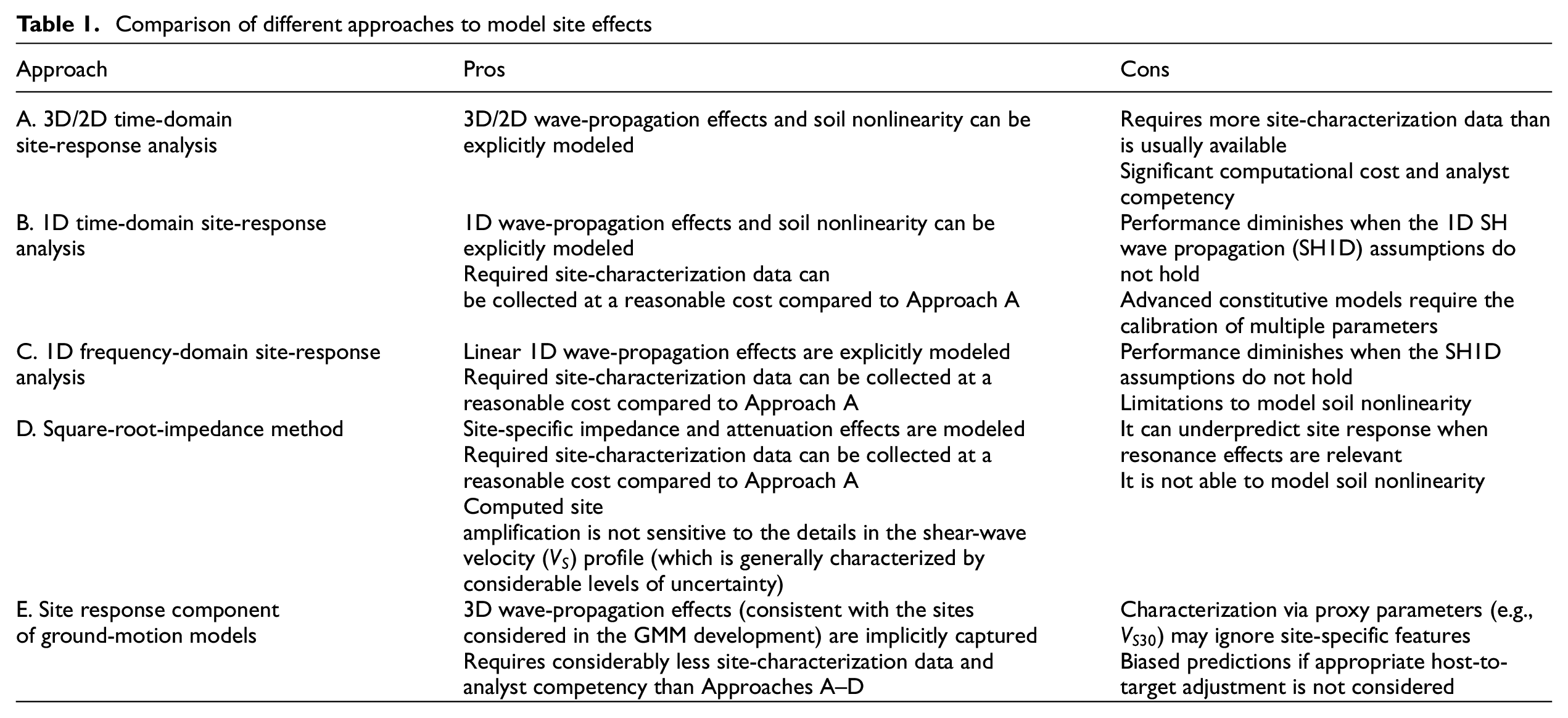
Approach A: 3D/2D time-domain site-response analysis
In this approach, the 3D or 2D wave equation is solved numerically (e.g. using finite element, finite difference, or spectral element methods) at different time steps, and soil nonlinearity is generally simulated using plasticity models (e.g. Yang et al., 2003). This method is the only one with the capability of explicitly simulating complex 3D/2D wave-propagation features such as basin effects (e.g. Ayoubi et al., 2021) or wave scattering due to soil heterogeneities (e.g. de la Torre et al., 2022a; Thompson et al., 2009), offering the highest potential to realistically simulate site effects among the approaches presented in Figure 1a. However, this would involve significant challenges in the model characterization, such as data collection within a great lateral extension (e.g. Hallal and Cox, 2023) or the definition of random-field (e.g. de la Torre et al., 2022b) and spatially distributed nonlinear parameters. Furthermore, defining an input motion on the model boundaries that adequately reflects the spatial variability of the incident wavefield can be challenging. This approach is not considered in the methods examined in this study to adjust ground-motion simulations.
Approach B: 1D time-domain site-response analysis
The numerical simulation in this approach relies on the 1D wave-propagation assumptions: the medium is represented by laterally continuous and homogeneous layers overlying a half-space; wavefronts are considered to be planar; and only horizontally polarized shear waves propagating in the vertical direction are modeled (the so-called SH1D assumptions). In addition to plasticity models, simpler cyclic stress-strain relationships (e.g. Groholski et al., 2016; Shi and Asimaki, 2017) can be used to capture soil nonlinearity. Adopting the SH1D assumptions has two implications: (1) it allows the problem to be represented with a relatively simple site-response model, and using site-characterization data (e.g. geophysical and cone penetration tests [CPTs]) that are typically collected within a relatively small area, corresponding to the site of interest, and (2) sites with conditions that violate these assumptions can result in inaccurate ground-motion predictions, as shown by several validation studies (e.g. Afshari and Stewart, 2019; Kaklamanos et al., 2013; Pilz and Cotton, 2019; Thompson et al., 2009, 2012; Zhu et al., 2022). As illustrated in Figure 1b, this approach is used in Method 5.
Approach C: 1D frequency-domain site-response analysis
This approach also relies on the SH1D assumptions. However, in this case, the problem is solved in the frequency domain through the direct application of a complex-valued transfer function,
Approach D: square-root-impedance method
This seismological approach combines the square-root-impedance (SRI) method (Boore, 2003, 2013; Joyner et al., 1981) to model site amplification,
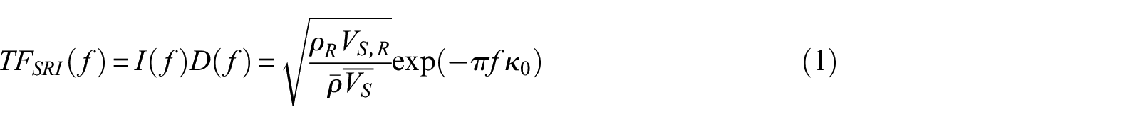
where
Several differences exist between
Approach E: site response component of a GMM
Semi-empirical GMMs (Baker et al., 2021, Ch. 4) provide a prediction of the mean value of a given intensity measure (IM) in natural log scale, for an earthquake rupture,

where

where
The terms
Hybrid broadband ground-motion simulation methodology
Overview
Currently, 3D numerical ground-motion simulations of the earthquake source and (3D) wave propagation are utilized in engineering applications only up to a limited maximum frequency of
The method developed by Graves and Pitarka (2010, 2015, 2016) (herein referred to as the GP method for brevity) has been applied and validated in different regions, including California, Europe, and New Zealand (e.g. Dreger et al., 2015; Lee et al., 2022; Razafindrakoto et al., 2021) and is considered in this article to illustrate the challenges in the modeling of shallow site effects in hybrid broadband simulations. In this method, the LF component is simulated using a kinematic description of the earthquake fault rupture and a visco-elastic finite-difference algorithm to solve the 3D wave propagation equation. The HF component is simulated using a stochastic representation of source radiation and a simplified Green’s function determined for a given 1D velocity structure. In particular, a frequency-dependent quality factor (
Considerations for the modeling of shallow site effects
The modeling of shallow site effects in hybrid broadband ground-motion simulations is usually performed using the “uncoupled approach” (e.g. de la Torre et al., 2020; Graves and Pitarka, 2010; Pilz et al., 2021; Razafindrakoto et al., 2021), and therefore, it takes the form of a posterior adjustment to the ground-motion time series produced by the regional-scale simulation. The four main aspects that need to be considered when performing this adjustment are discussed below.
First, the hybrid nature of the simulation method requires different considerations for the adjustment of the LF and HF components. For example, in the case of the GP method, the 3D velocity structure considered in the LF approach allows for the incorporation of any level of spatial variability within the simulation domain, whereas the HF approach is usually performed using a unique 1D velocity profile representative of the whole region of interest (e.g. Graves and Pitarka, 2010; Lee et al., 2022). Consequently, the 1D velocity profile implicit in the LF and HF components of the simulated ground motions at a given site can be significantly different, including the minimum
Second, due to knowledge and computational limitations, the minimum
Third, although near-surface sediments are generally not properly modeled in the regional-scale simulation (e.g. due to the high
Finally, regional-scale simulations are usually performed considering linear viscoelastic materials (e.g. Graves and Pitarka, 2010; Lee et al., 2022). Hence, the adjustment has to model soil nonlinearity, which is particularly relevant for maximum shear strains
Case study
General description
A case study is considered to examine the different methods to adjust ground-motion simulations and compare and contrast their features. It includes four strong motion station (SMS) sites in Christchurch, New Zealand, for which site characterization data (e.g. Teague et al., 2018; Wotherspoon et al., 2015) and simulation results of historical events (Lee et al., 2022; Razafindrakoto et al., 2018) are available. Table 2 shows that the four sites represent a wide range of site conditions.
Parameters representative of the actual and simulation site conditions for the four sites considered
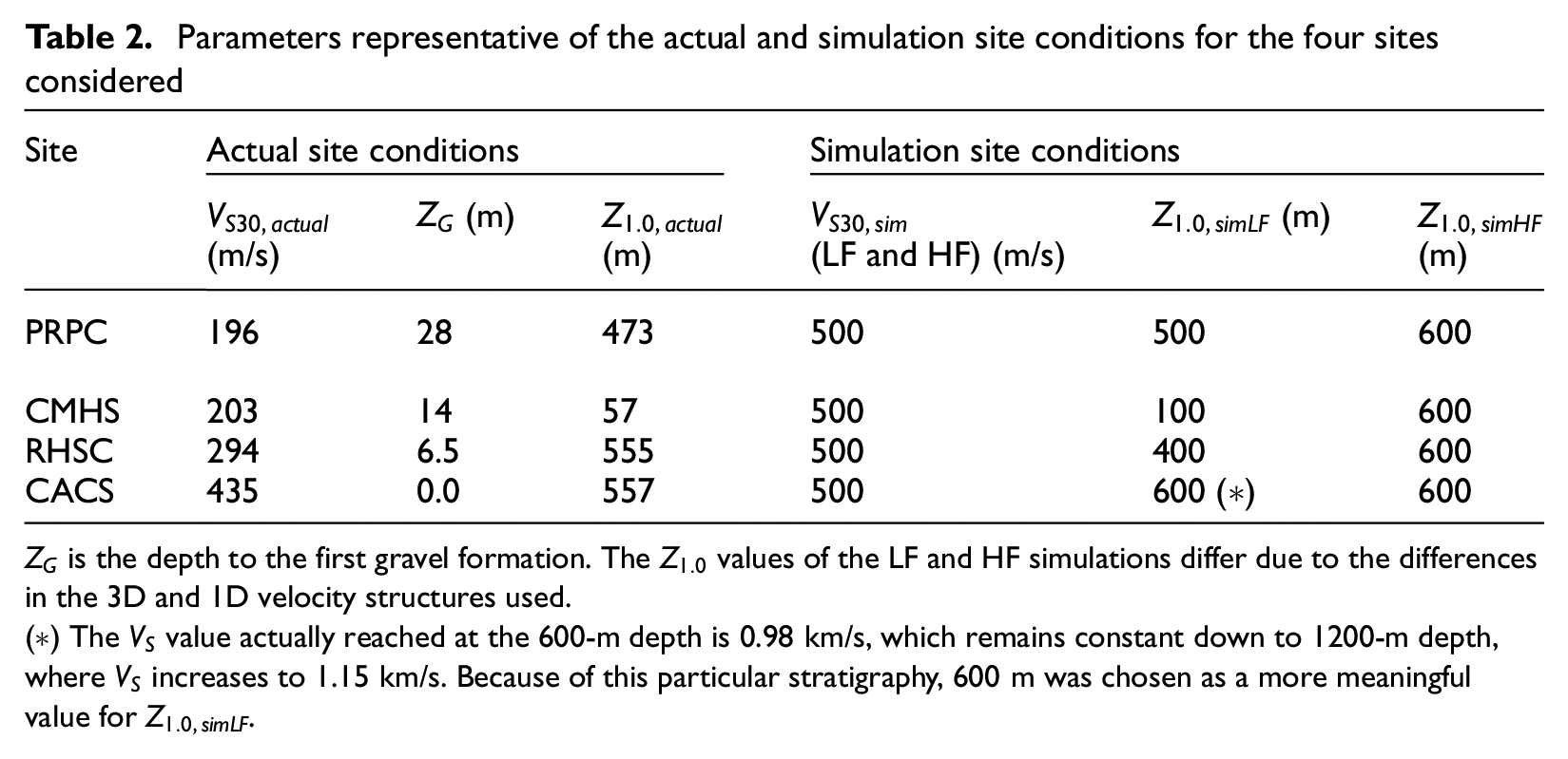
A low- and a high-intensity ground motion are considered for each site in order to examine the different methods in the near-linear and nonlinear response regimes. The associated events are described in Electronic Supplement A. Only one horizontal component of these ground motions is used.
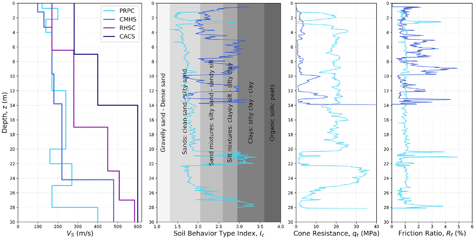
Site-characterization data
Figure 2 presents the
Ground-motion simulations considered
The events considered in this case study were simulated using the GP method. The simulations of the low-intensity events were performed by Lee et al. (2022), and those of the high-intensity event by Razafindrakoto et al. (2018). For the LF component, the NZVM (Thomson et al., 2020) v2.02 with a grid spacing of 100 m and a minimum
Figure 3a shows the 1D
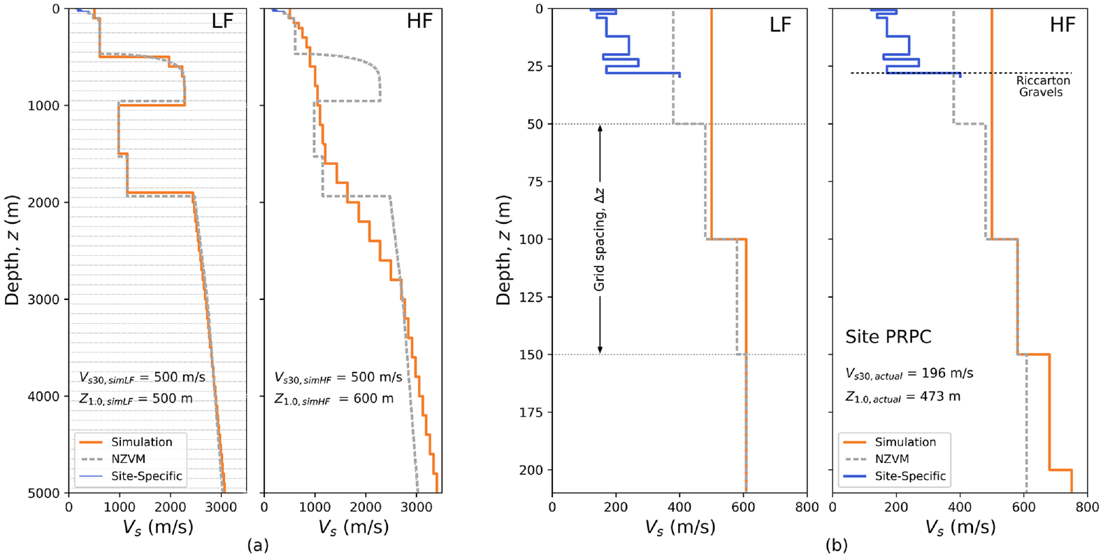
Site-specific, LF simulation, HF simulation, and NZVM (v2.07)
Methods for performing site adjustments to hybrid broadband ground-motion simulations
Overview
In this section, five methods to perform the site adjustment are presented, and the case study sites are used to illustrate their application and compare the methods under different soil conditions. As shown in Figure 1b, these methods are based on a range of different approaches discussed in the “Approaches for modeling local site effects” section; in particular, Approaches B–E. Approach A was not considered in this study because its use in engineering applications is limited. For example, even though the sites considered in the case study are well-characterized near the SMS, proper implementation of Approach A would require spatially distributed data over a considerably larger area (Hallal and Cox, 2023), and these data are significantly sparser. Also, defining an input motion that is compatible with the regional-scale ground-motion simulation is challenging. While methods exist that allow determining the equivalent input forces derived from 3D ground-motion simulations (e.g. Bielak, 2003), their implementation requires significant analyst competency and dealing with the hybrid nature of the simulation method.
The site adjustment can be performed in the frequency domain (Methods 1–4) or in the time domain (Method 5). The “frequency-domain adjustment” involves five steps:
Obtaining the simulated acceleration time series at the surface of the site of interest,
Computing the discrete Fourier transform (DFT) of
Determining the SF to be applied to account for shallow site effects. SF is defined as a function of frequency, and Methods 1–4 represent different formulations to obtain it. In these methods, only an amplitude adjustment is considered (i.e. the phase of the simulated ground motion is not modified), but a phase adjustment can also be included (e.g. Pilz et al., 2021; Shi, 2019), which would account for the time delay of the seismic waves when propagating through the soil deposit. This phase adjustment could be relevant in the analysis of spatially distributed infrastructure (Shi, 2019: Ch.4).
Applying the SF to the DFT of
Obtaining the adjusted acceleration time series (which accounts for shallow site effects),
Since the simulated acceleration time series are different for the LF and HF components, the adjustment is performed separately for each component, and then the adjusted LF and HF time series are combined in the time domain. This procedure is described in the “Application of the site factor” section of Electronic Supplement B. Given that the simulation profiles are also different for each component, this may result in different LF and HF SFs. In the following sections describing Methods 1–4, the LF and HF SFs are only plotted in their associated frequency ranges (
The “time-domain adjustment” involves the use of time-domain site response analysis. Method 5 corresponds to a specific implementation of this approach, based on 1D nonlinear inelastic site-response analysis, and it is further explained in the “Method 5 - 1D time-domain wave propagation analysis” section.
The site PRPC is first used to explain the methods, but results for all four case study sites are provided in Electronic Supplement C and in the “Comparison of the site amplification obtained with the five methods” section.
Method 1—
-based amplification
This method uses the site response scaling factor (
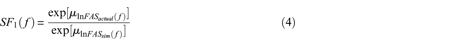
Since semi-empirical models for FAS have only recently been developed (e.g. Bayless and Abrahamson, 2019; Bora et al., 2019), several previous studies have used GMMs for SA to approximately compute
Since source and path effects are common to the numerator and denominator in Equation 4, it reduces to the ratio of site terms. Specifically:

where all terms have been previously defined in the “Approach E: Site response component of a ground-motion model” section. The terms

This results in a SF that can be expressed as,

where
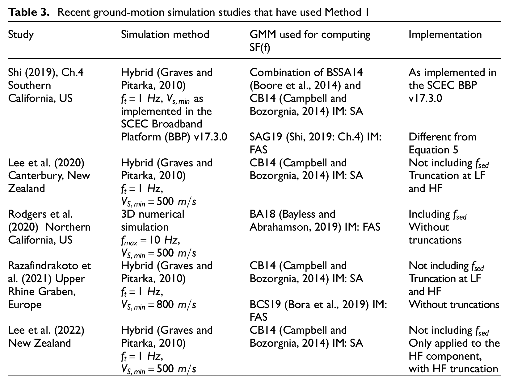
Table 3 summarizes some of the most recent studies on ground-motion simulations where Method 1 has been used to capture site effects. The table illustrates that there is no consistent approach to date to implement Method 1, and subjective decisions are involved in the selection of the GMM, the application of LF and HF truncations, and the inclusion of the
Recent ground-motion simulation studies that have used Method 1
In order to illustrate the implications of alternative combinations of models, Figure 4 presents the resulting SFs (
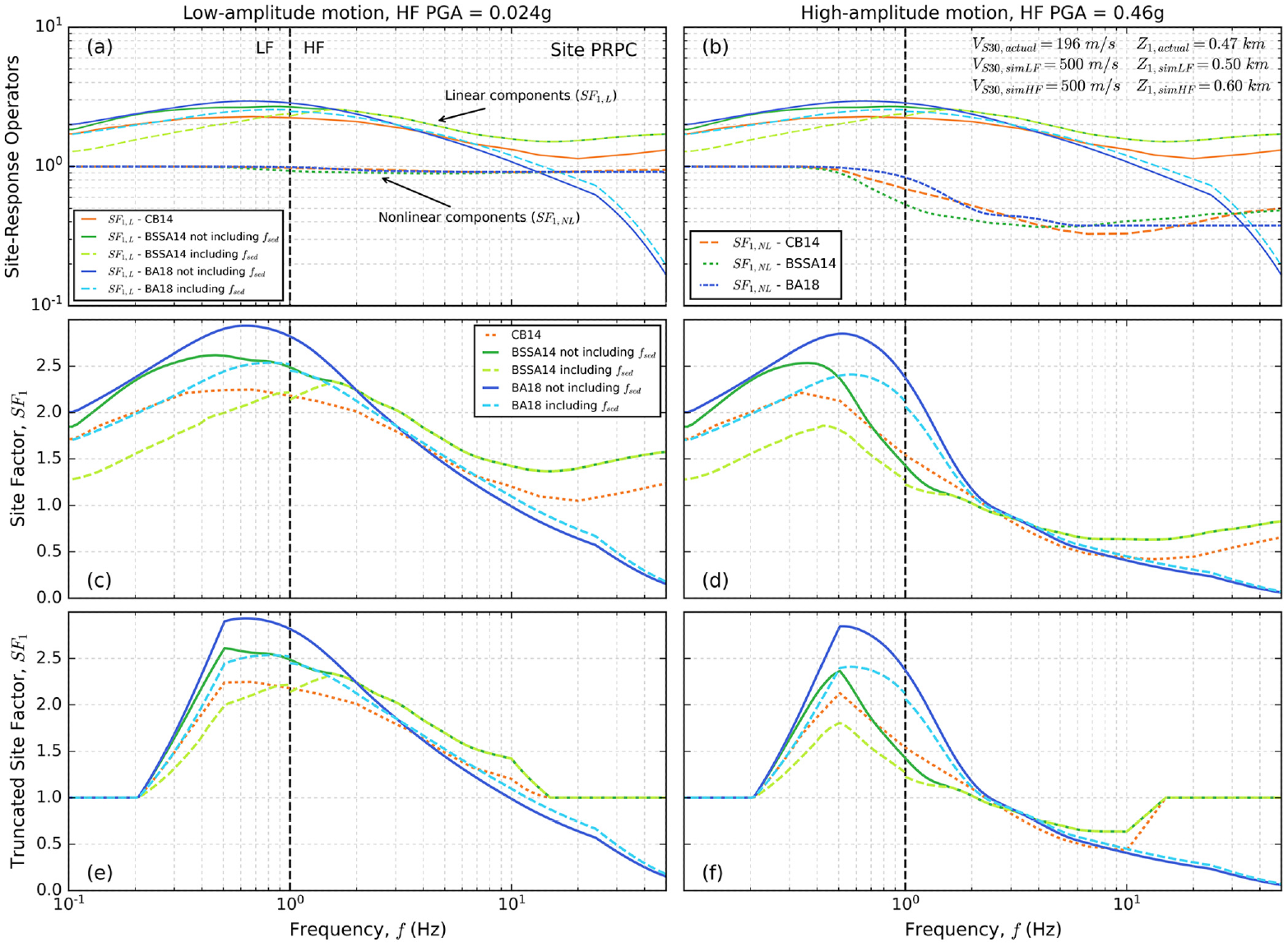
Site factors obtained for the site PRPC using Method 1 and different models: (a) and (b) Show the linear and nonlinear components for the low-amplitude and high-amplitude motion, respectively. (c) and (d) Present the resulting site factors without any truncations. (e) and (f) Show the site factors with LF and HF truncations.
Figures 4a and b display the linear (
Significant model-to-model variability is observed in the linear and nonlinear components of the SF in Figures 4a and b, but in the latter case, this variability only manifests under the high-amplitude ground motion (Figure 4b). For the low-amplitude motion, the nonlinear component of the three GMMs is close to unity over the entire frequency range, whereas for the high-amplitude motion, this component substantially departs from 1 at frequencies greater than 0.5 Hz, resulting in de-amplification. These figures also show that the BA18 model accounts for the HF decay in the site response, a feature that cannot be properly captured in the response spectral domain (Bora et al., 2016; Cabas and Rodriguez-Marek, 2017).
A common feature observed in all the SFs, clearly illustrated in Figures 4c and d, is the relatively high amplification at low frequencies, particularly around
Host-to-target adjustment issue
To investigate the root cause of the apparent overamplification at relatively low frequencies, Figure 5a illustrates a
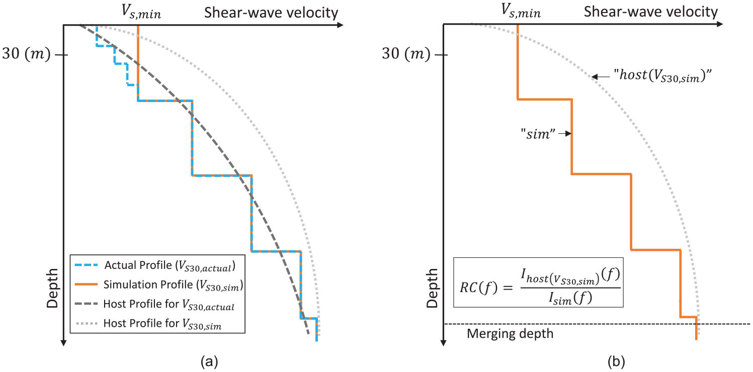
(a) Illustration of the host-to-target conversion issue present in Method 1. (b) Computation of the reference correction (RC) factor introduced in Method 2.
Figure 5a illustrates that a significant inconsistency may exist between the “target” condition to be modeled (i.e. relative site response between the actual and simulation profile) and the “host” condition implicit in the SF
Inconsistency between the simulation profile and the host profile for
Inconsistency between the actual profile and the host profile for
Double-counting deep 3D velocity structure effects: If the ground-motion simulation is conducted using a high-quality 3D velocity model for the LF component, it will be possible to capture 3D amplification phenomena, including basin effects, which means that the SF does not have to account for them. However, since the host profile for
Method 2—
-based amplification with host-to-target adjustment
In Method 2, a host-to-target adjustment is proposed to partially overcome the inconsistency involved in Method 1. Particularly, this adjustment addresses the first issue explained in the previous section (“Host-to-target adjustment issue”), related to the difference between the simulation profile and the host profile for

where
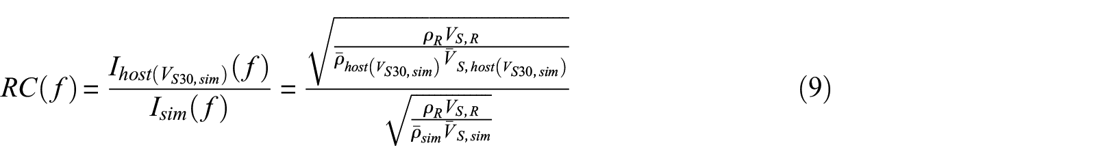
where the subscripts
The main challenge for the application of Method 2 is deriving the host profile implicit in the GMM(s) considered for
Figure 6 presents the computation of the reference correction factor for the site PRPC, considering the CB14 model (results for the BSSA14 model are provided in Electronic Supplement C). As shown in Figure 6a, the different LF and HF simulation profiles result in slightly different merging depths at each frequency range. Given that the accuracy of the host profile estimation reduces with depth, this profile was modified to be equivalent to the simulation profile below the selected merging depth. The reference depth for the calculating
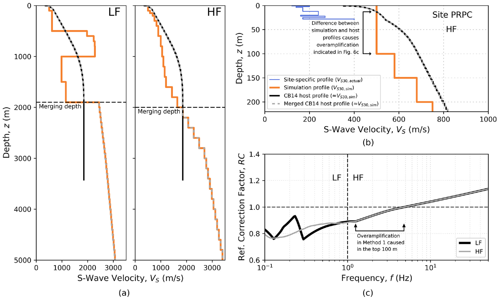
Reference adjustment in Method 2 for the site PRPC: (a) LF and HF profiles, from 0 to 5000 m; (b) HF profiles from 0 to 220 m; and (c) resulting reference correction factors.
Figure 6c shows that the resulting reference correction factor is less than 1 for
Method 3—SRI-based amplification
Methods 1 and 2 only require proxy parameters (e.g.
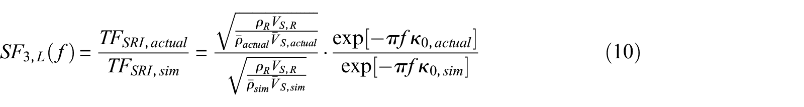
where the subscripts
The objective of the denominator in Equation 10 is to remove the impedance- and attenuation-based site response introduced by the regional ground-motion simulation within the depth over which the site adjustment is considered. The use of the SRI method in this equation is fully consistent with the treatment of the linear amplification and HF attenuation adopted in the HF ground-motion simulation method (as described in the “Hybrid broadband ground-motion simulation methodology” section). Although the LF simulation is based on a different approach (3D time-domain wave propagation), the frequencies affected by
Equation 10 can be rewritten as
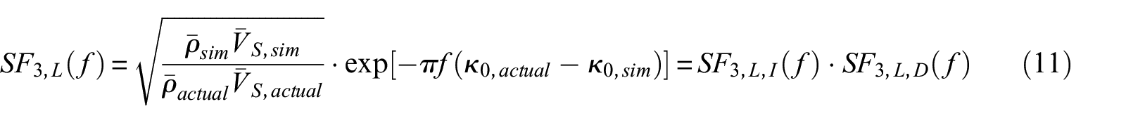
where
Since Equation 11 (i.e. Approach D) is limited to the estimation of the linear site response, the nonlinear operator derived in Method 1 is proposed for capturing soil nonlinearity in Method 3. In this way, the total SF in Method 3 (

Figure 7 illustrates the computation of the linear component of Method 3 for the site PRPC. Figure 7a shows the derivation of the actual
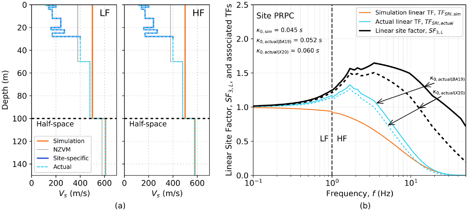
(a)
Since the HF ground-motion simulation methodology uses the SRI method in the same fashion as Method 3,
Figure 8 presents the SFs (
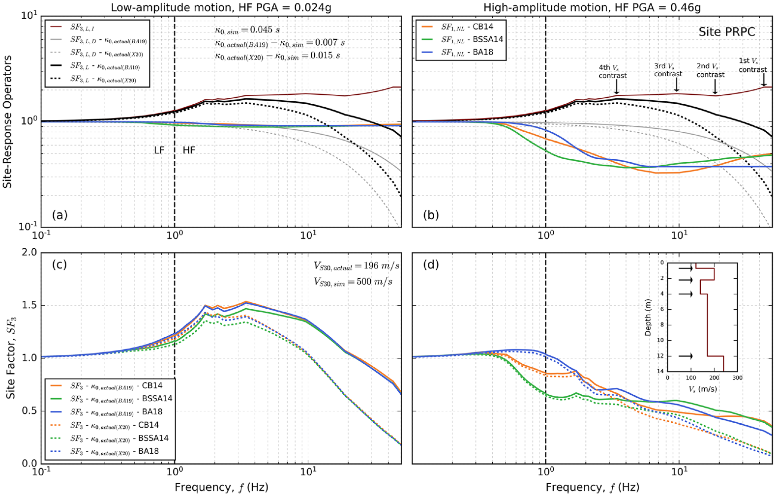
(a) Site-response operators of Method 3 for the site PRPC considering the low-amplitude motion, (b) the high-amplitude motion, (c) resulting site factors for the low-amplitude motion, and (d) high-amplitude motion.
Method 4—1D TF-based amplification
Method 4 is similar to Method 3 but uses the theoretical 1D TF (Approach C) to account for linear site effects. The linear component of the SF can be expressed as follows:
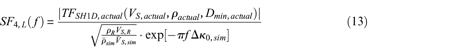
where the numerator represents the linear site response for the actual profile, computed through the modulus of the outcrop 1D TF (
In the same manner as in Method 3, nonlinearity is modeled in Method 4 using the nonlinear operator from Method 1. Hence, the total SF in Method 4 (

Other studies have also utilized theoretical 1D TFs to adjust hybrid broadband ground-motion simulations (e.g. Ojeda et al., 2021; Pilz et al., 2021), but either they have not accounted for soil nonlinearity (e.g. Ojeda et al., 2021) or have used a different approach to model it, such as the equivalent linear method (e.g. Pilz et al., 2021). The method proposed here to treat nonlinearity along with the linear amplification from the 1D TF is simpler and only requires
Several approaches have been proposed to estimate the small-strain damping
In the case of Method 3, the parameter

where
Figure 9 illustrates the computation of the linear component of Method 4 for the site PRPC. Figure 9a shows the
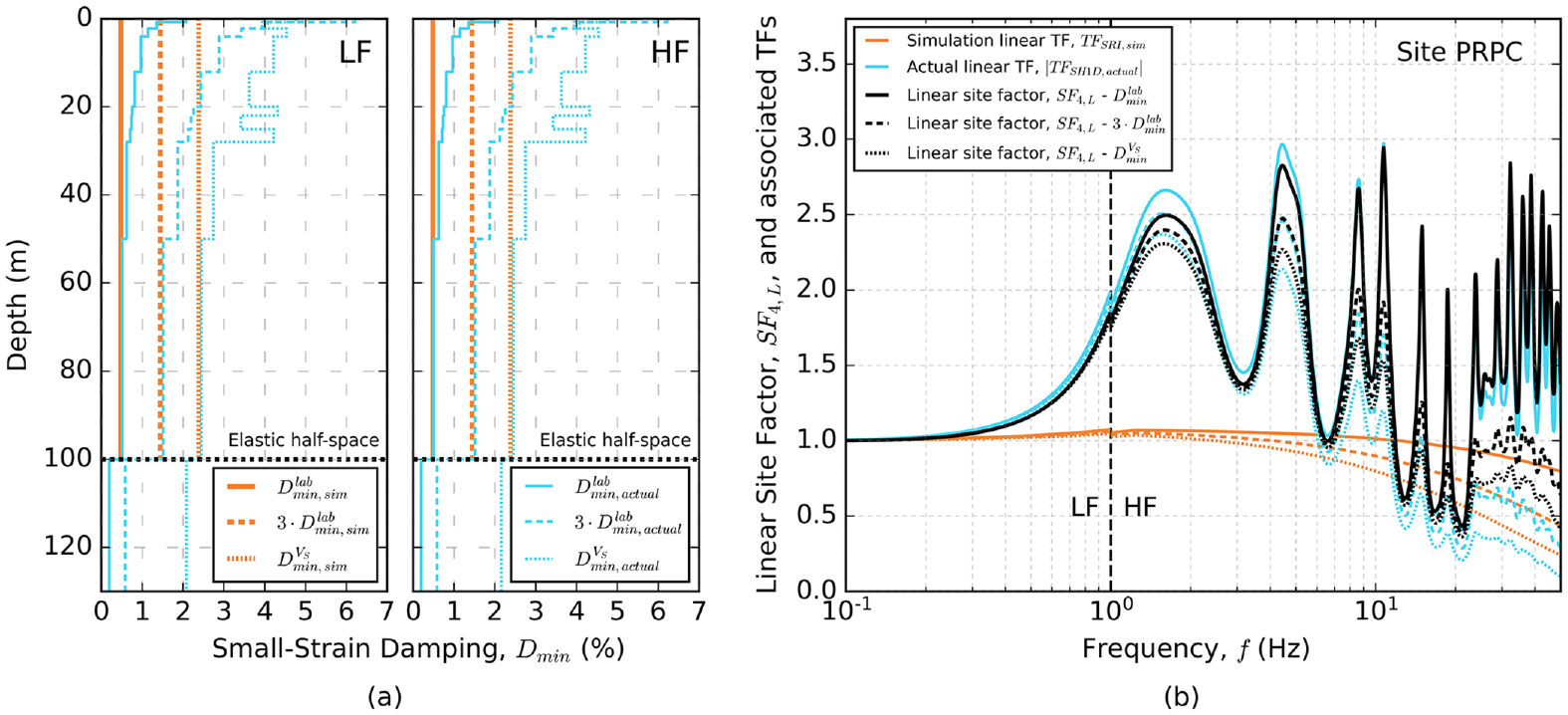
(a)
Figure 10 shows the SFs (
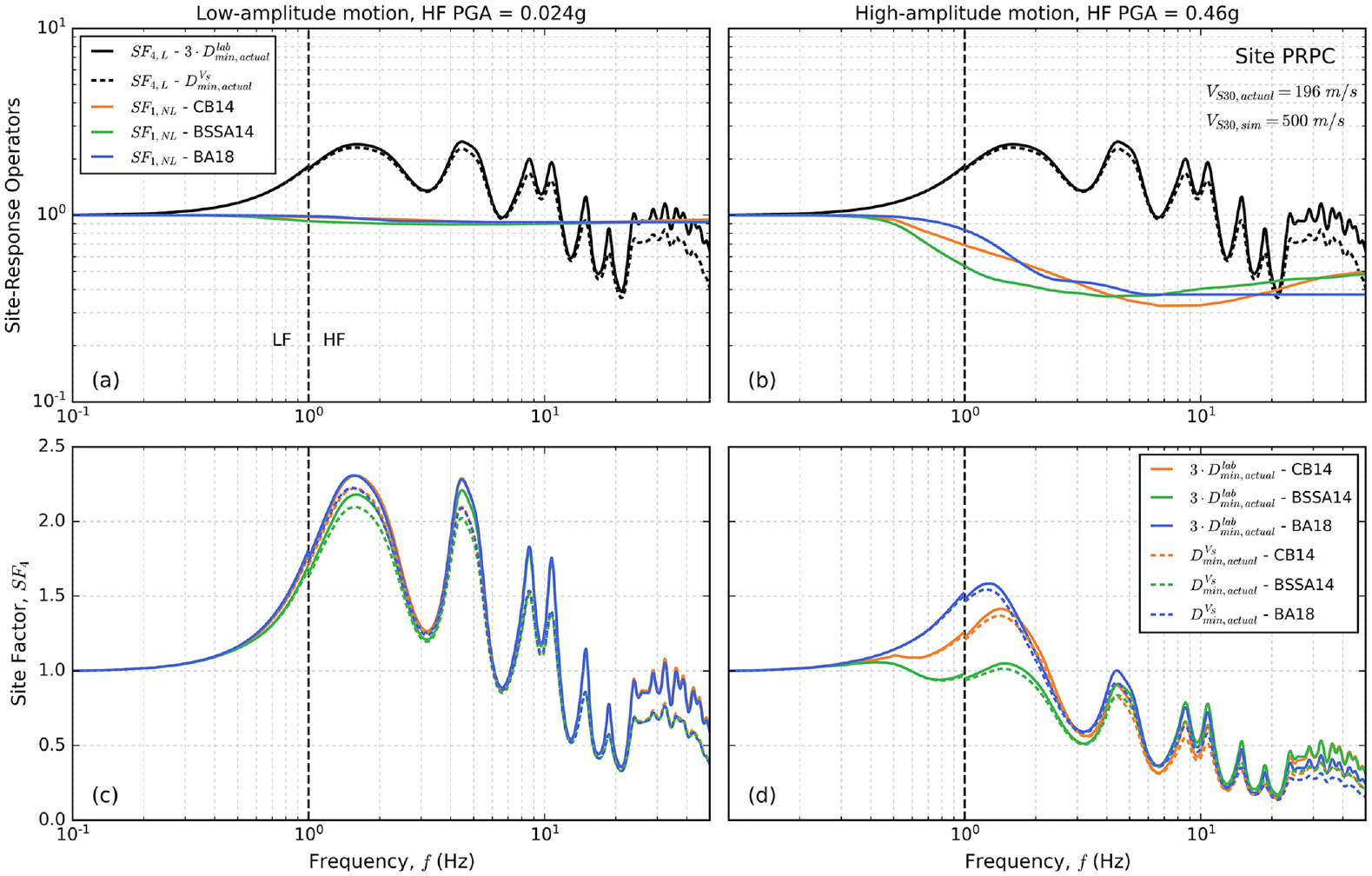
(a) Site-response operators of Method 4 for the site PRPC considering the low-amplitude motion, (b) the high-amplitude motion, (c) resulting site factors for the low-amplitude motion, and (d) high-amplitude motion.
Method 5—1D time-domain wave propagation analysis
Method 5 is a two-step procedure that generally requires more site-characterization data than Methods 3 and 4. Similar to Method 4, it relies on the SH1D assumptions but uses 1D time-domain wave propagation analysis (Approach B) to capture the near-surface nonlinear site response. In this method, the actual profile is divided into two portions: the “actual 1” and “actual 2” profiles. As illustrated in Figure 11a, for the site PRPC, the actual 2 profile corresponds to the shallower portion, which is bounded by a significant impedance contrasts at the bottom (corresponding to the top of the Riccarton Gravel Formation, characterized by
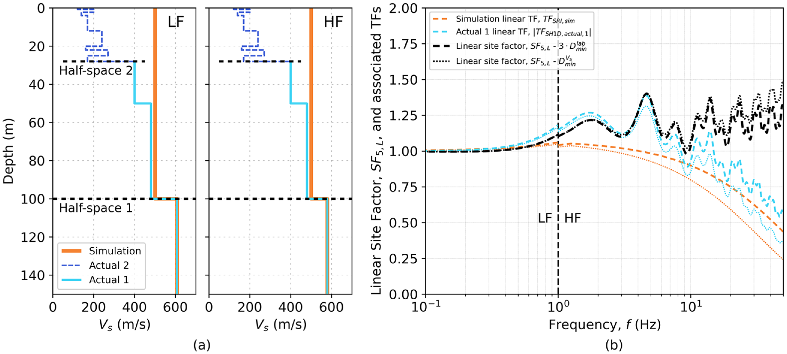
(a)
Figure 12 illustrates Method 5. In Step 1, a linear SF,
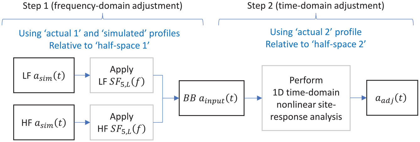
Illustration of Method 5. In Step 1, a frequency-domain adjustment is performed to the LF and HF simulated ground motions (
The main reason for computing the site-response of the actual profile in two steps (i.e. using the actual 1 and 2 profiles) is to deal with different half-space 1 properties for the LF and HF components. In the case of the site PRPC, the difference between LF and HF
For the 1D time domain site-response analysis, different codes (Hashash et al., 2020; Jsh9, 2023; McKenna, 2011) and constitutive models (Groholski et al., 2016; Shi and Asimaki, 2017; Yang et al., 2003) were used to investigate the impact of alternative modeling decisions on the resulting site adjustment. The results of these analyses, summarized in the “Method 5” section of Electronic Supplement C, show that when the comparison is performed in a consistent manner (i.e. using the same modulus reduction (MR) curves), the variability in the site adjustment is significantly reduced. Therefore, in the following section, the results for Method 5 are only provided for the case in which the program OpenSees (McKenna, 2011) is used, along with the constitutive models PressureDependMultiYield02 and PressureIndependMultiYield (Yang et al., 2003, 2008), and user-defined MR curves. The MR curves were defined based on the Darendeli (2001) model, with a large-strain adjustment (Yee et al., 2013) for consistency with the soil shear strength. The estimation of the soil properties (e.g. actual soil density, PI, friction angle, and undrained shear strength) was based on the
Comparison of the site amplification obtained with the five methods
Prior figures for each method focused on intra-method differences due to input parameter and model alternatives, using the site PRPC as an example. This section provides a comparison between the five methods for all four case study sites. Figure 13 presents a comparison of the linear SFs (
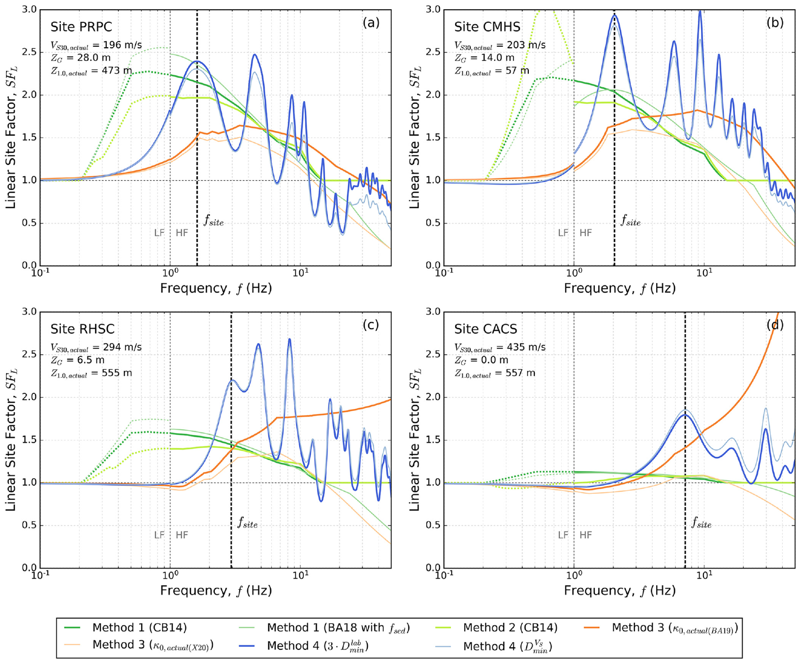
Comparison of the linear factors obtained with Methods 1–4 for the sites: (a) PRPC, (b) CMHS, (c) RHSC, and (d) CACS. Dashed lines in Methods 1 and 2 indicate that the LF component is not used in the adjustment.
Figure 13 shows that in the four sites investigated, the linear SFs obtained with Methods 3 and 4 mainly affect the HF range and tend to a value of 1 at low frequencies, reflecting the fact that the adjustment is only accounting for shallow site effects (within the top 100 m); whereas Methods 1 and 2 generally produce considerable amplification in the LF range. Following this, and considering that the compatibility with the regional-scale simulation is explicitly controlled in Methods 3 and 4, in the case of Methods 1 and 2, the SF is only applied to the HF simulation component (such as in Lee et al., 2022). The implementation of this procedure is described in Electronic Supplement B. Figure 13 suggests that the frequency range of application of these SFs should be defined in a site-specific manner, but for Methods 1 and 2, it is assumed that a site-specific
In the case of the four sites considered, Method 1 produces higher amplification than Methods 3 and 4 in the vicinity of
The ergodic assumption implicit in Method 1 is illustrated when comparing the linear SFs for the sites PRPC and CMHS. These two sites are characterized by very similar
Method 4 produces significant variations in the SFs over narrow frequency bands, whereas Method 3 results in SFs varying smoothly with frequency. In particular, Method 4 generates significantly greater amplification than Method 3 around
Figure 13 illustrates that the definition of
Figures 14 and 15 present the AFs, which now include the influence of nonlinearity, that result from applying Methods 1–5 to the four sites investigated, for the low- and high-amplitude ground motion, respectively. For a given IM, AF is defined as

where
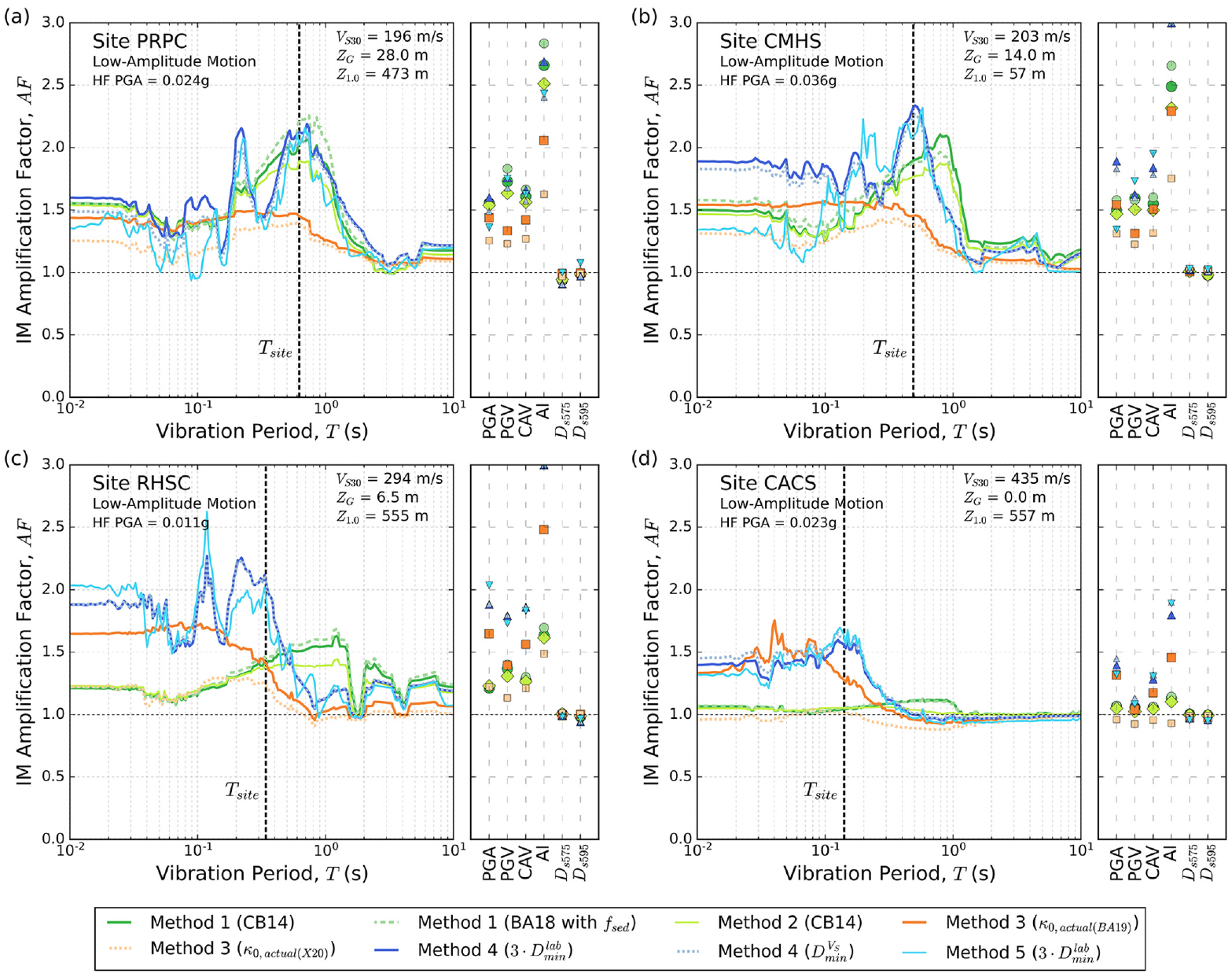
Amplification factors of different IMs resulting from applying Methods 1–5 to the sites: (a) PRPC, (b) CMHS, (c) RHSC, and (d) CACS, for the low-amplitude ground motion. For visual completeness, the AI AFs for the sites CMHS and RHSC associated with Methods 4 and 5 are plotted at the vertical axis limit (3.0). The actual values for CMHS are 3.45 (Method 4 using

Amplification factors of different IMs resulting from applying Methods 1–5 to the sites: (a) PRPC, (b) CMHS, (c) RHSC, and (d) CACS, for the high-amplitude ground motion.
In the case of the low-amplitude motion (Figure 14), which produces relatively low levels of soil nonlinearity, the response spectral amplification generally follows a shape and amplitude similar to the linear SFs plotted in Figure 13 in the intermediate period range (approximately 0.1 <
Figure 14 also shows that Method 4 and 5 generally display similar shapes and amplitudes in the response spectral AF for the low-amplitude motions, which is expected given that both methods rely on 1D site-response analysis. However, at some vibration periods, considerable differences are observed due to the different treatment of nonlinear site-response, the use of more site-specific data, and the decoupling of the site-response analysis in Method 5. For example, for the site CMHS, at very short vibration periods, Method 5 results in considerably lower values of amplification. This is mainly due to the more significant soil nonlinearity predicted by Method 5, which is modeled in a site-specific fashion, accounting for the relatively low values of cone resistance at this site (see Figure 2).
AI displays particularly high levels of amplification and method-to-method variability in Figure 14, especially in the case of the softer sites. On the other hand, the significant durations
Figure 15 shows that for the high-amplitude motion considered, soil nonlinearity has a strong influence on AF, especially for the softer sites, PRPC, and CMHS. At these sites, severe de-amplification is observed at short-period SAs, PGA, and AI, and amplification is generally produced in the significant durations
Discussion
Table 4 summarizes the main advantages and disadvantages of the five methods investigated and illustrates important trade-offs between them. Going from Method 1 to Method 5 involves the use of increasing levels of site-characterization data and more location-specific treatment of the site adjustment.
Comparison between five methods investigated
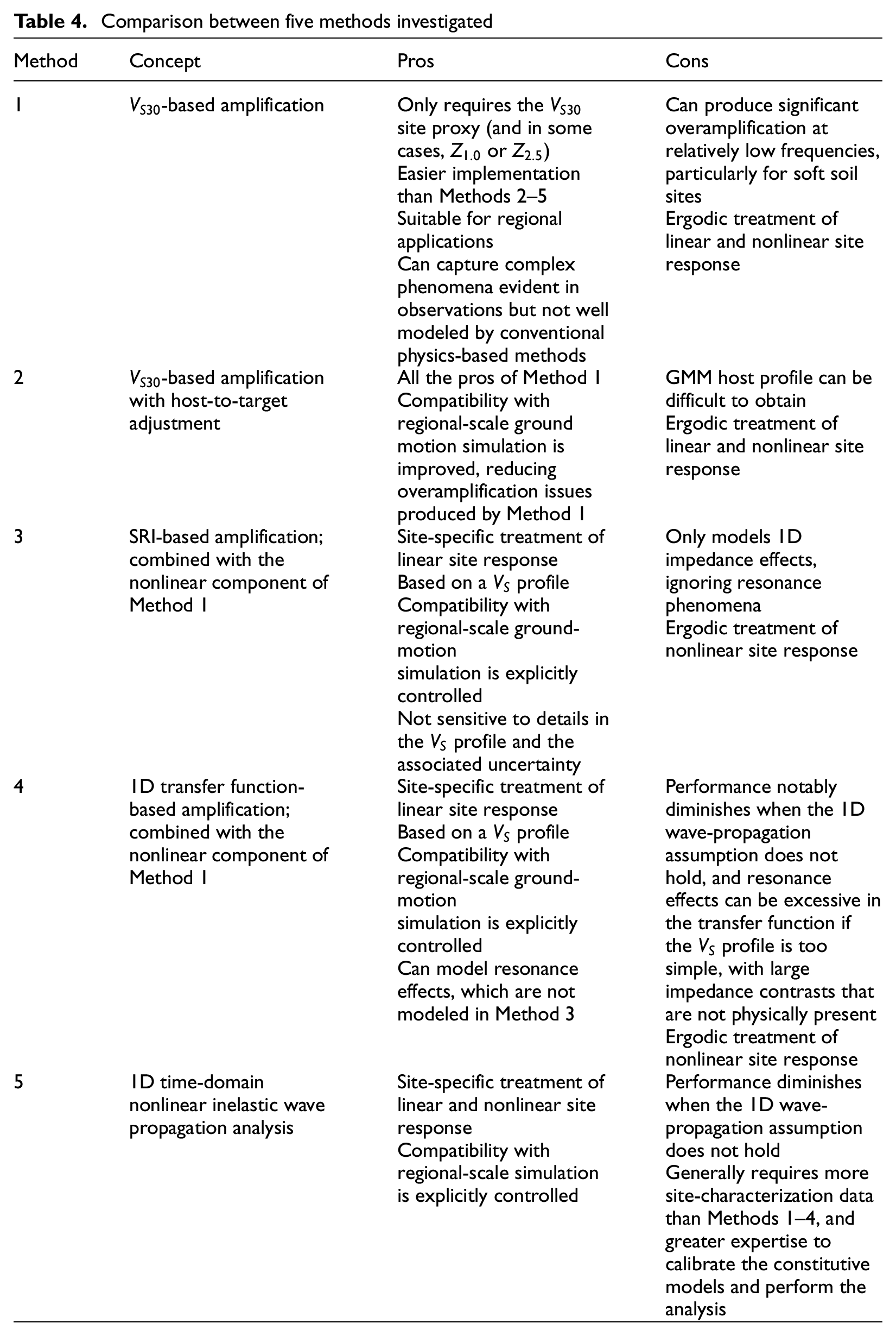
Other than the simplicity and small requirement of site information (which is ideal for regional applications), the only conceptual advantage of Methods 1 and 2 is their ability, via empirical calibration, to implicitly capture complex phenomena observed in reality that are difficult to explicitly model using physics-based methods. It is worth noting that although Methods 3–5 make use of physics-based approaches and additional site-specific data, these approaches are limited to the use of a 1D representation of the soil profile, and hence, they are unable to explicitly model 3D effects. However, the actual characteristics of these 3D effects are region- and site-specific, which may limit the ability of Methods 1 and 2 to offer a significant advantage, especially in regions other than those for which the empirical models were calibrated. Another related situation where Method 1 can produce beneficial effects is when it compensates for unmodeled phenomena in the regional-scale simulation. For example, although the LF simulation in the GP method explicitly models 3D effects, its ability to properly capture them strongly depends on the quality of the velocity model considered. Method 1 implicitly captures site effects associated with the deep velocity structure of a site (e.g. basin effects and impedance-based amplification associated with deep layers), which can result in strong amplification at relatively low frequencies when compared with the other methods, especially for sites with low
Method 2 partially deals with the host-to-target adjustment issue present in Method 1 and can reduce the Method 1 overamplification in both the LF and HF range. However, the resulting amplification in the LF range may still be significantly higher than that obtained from Methods 3–5 for relatively soft sites. This limited effect of Method 2 on low frequencies may be due to basin effects implicit in the GMM, which are not removed by this method; challenges associated with the determination of an accurate 1D host profile, required in Method 2; and limitations of the SRI method, which is used to compute the reference correction factor.
Methods 3–5 explicitly control the compatibility with the regional-scale simulation. The effects produced by the simulation in the shallow portion of the site are removed and modified in a site-specific manner, which avoids the host-to-target adjustment issue present in Method 1, and to a lesser extent, Method 2. Also, in contrast to Methods 1 and 2, these methods explicitly model the site-response physics to different extents using a 1D representation of the site. Therefore, the suitability of this representation, along with the quality of the site-characterization data, will determine the performance of these methods, especially in the case of Methods 4 and 5 which more strongly rely on the SH1D assumptions. Evidence suggests that these assumptions may only hold for a modest percentage of cases (e.g. Afshari and Stewart, 2019; Thompson et al., 2012), and even for such “1D” sites, 1D site-response analysis can be inaccurate (Pretell et al., 2023). Because of this, several approaches have been proposed to adjust 1D site-response analysis to implicitly account for spatial variability and other unmodeled phenomena (e.g. Hallal et al., 2022; Pretell et al., 2023). However, their capacity to improve predictions is generally limited to 1D-like sites. Thus, advancing the use of a time-domain adjustment with 2D or 3D site-response analysis (e.g. de la Torre et al., 2022a, 2022b; Hallal and Cox, 2021) may be required to significantly improve predictions at complex sites, which would involve the collection of further site-characterization data, and to properly address the compatibility issue between the regional simulation and the 2D/3D site-response model.
The aforementioned discussion illustrates that it is not possible to determine a priori the best method to adjust hybrid broadband ground-motion simulations. The quality of the regional velocity model; characteristics of the site and its location within the sedimentary basin and relative to earthquake source (e.g. Smerzini et al., 2011); and site-characterization data available will dictate which method is the most appropriate to use. This highlights the need for systematic validation of alternative methods against observations (e.g. Kuncar et al., 2024) to inform method and model selection in forward applications.
Conclusions
This article presented a comprehensive examination on the incorporation of shallow site effects in hybrid broadband ground-motion simulations. Five methods were presented that allow for the adjustment of ground-motion time series produced by regional simulations to account for unmodeled site effects and represent a wide range of options in terms of the site-characterization data and expertise required. The methods were applied to four sites representative of different soil conditions, and two levels of ground-motion amplitude were considered, to investigate the relative adjustment that they can generate on different IMs.
The results show that significant variability exists in the SFs and IM amplifications predicted by the different methods. Method 1 (
Methods 3 and 4 were proposed as alternatives when a
Several sources of parametric and modeling uncertainty are involved in each method, which can produce considerable within-method variability as shown by the sensitivity analyses performed in this study. In particular, the definition of
Advances in computational capability, theory, and knowledge will allow for explicitly modeling shallow site effects in 3D numerical simulations, but this progress will be region-specific. In the interim, the methods presented in this article can be used in engineering applications, and this study can help to clarify their limitations and the impact of different modeling decisions. To evaluate the relative performance of these methods under a diverse range of earthquake sources, site conditions, and site-characterization data, direct comparison with observations from multiple sites and events is needed.
Supplemental Material
sj-csv-2-eqs-10.1177_87552930241301059 – Supplemental material for Methods to account for shallow site effects in hybrid broadband ground-motion simulations
Supplemental material, sj-csv-2-eqs-10.1177_87552930241301059 for Methods to account for shallow site effects in hybrid broadband ground-motion simulations by Felipe Kuncar, Brendon A Bradley, Christopher A de la Torre, Adrian Rodriguez-Marek, Chuanbin Zhu and Robin L Lee in Earthquake Spectra
Supplemental Material
sj-csv-3-eqs-10.1177_87552930241301059 – Supplemental material for Methods to account for shallow site effects in hybrid broadband ground-motion simulations
Supplemental material, sj-csv-3-eqs-10.1177_87552930241301059 for Methods to account for shallow site effects in hybrid broadband ground-motion simulations by Felipe Kuncar, Brendon A Bradley, Christopher A de la Torre, Adrian Rodriguez-Marek, Chuanbin Zhu and Robin L Lee in Earthquake Spectra
Supplemental Material
sj-pdf-1-eqs-10.1177_87552930241301059 – Supplemental material for Methods to account for shallow site effects in hybrid broadband ground-motion simulations
Supplemental material, sj-pdf-1-eqs-10.1177_87552930241301059 for Methods to account for shallow site effects in hybrid broadband ground-motion simulations by Felipe Kuncar, Brendon A Bradley, Christopher A de la Torre, Adrian Rodriguez-Marek, Chuanbin Zhu and Robin L Lee in Earthquake Spectra
Footnotes
Acknowledgements
The authors thank Linda Al Atik for providing the host profiles that were used to illustrate the application of Method 2, and Sean Ahdi and two anonymous reviewers for providing valuable comments on the manuscript. The authors would also like to gratefully acknowledge the New Zealand eScience Infrastructure (NeSI) and the Korea Institute of Science and Technology Information (KISTI) [KSC-2023-CRE-0459] for the high-performance computing resources provided.
Declaration of conflicting interests
The author(s) declared no potential conflicts of interest with respect to the research, authorship, and/or publication of this article.
Funding
The author(s) disclosed receipt of the following financial support for the research, authorship, and/or publication of this article: This work was financially supported by the University of Canterbury, QuakeCoRE: The NZ Center for Earthquake Resilience, Resilience to Nature’s Challenges National Science Challenge, the Marsden Fund, and the New Zealand Natural Hazards Commission (Toka Tū Ake). This is QuakeCoRE publication number 978.
ORCID iDs
Data and resources
Figures 1, 5, and 12 were prepared using Microsoft PowerPoint, and the remaining figures were generated in Python (https://www.python.org/). The host profiles derived by Linda Al Atik (personal communication, April 6, 2023), that were used to illustrate the application of Method 2, are provided in the Supplemental Material. The New Zealand Velocity Model (NZVM) code is available at ![]() .
.
Supplemental material
Supplemental material for this article is available online.
References
Supplementary Material
Please find the following supplemental material available below.
For Open Access articles published under a Creative Commons License, all supplemental material carries the same license as the article it is associated with.
For non-Open Access articles published, all supplemental material carries a non-exclusive license, and permission requests for re-use of supplemental material or any part of supplemental material shall be sent directly to the copyright owner as specified in the copyright notice associated with the article.