Sage Journals: Discover world-class research

Abstract

In site-specific site-response assessments, observation-based site-specific approaches requiring a target–reference recording pair or a regional recording network cannot be implemented at many sites of interest. Thus, various estimation techniques have to be used. How effective are these techniques in predicting site-specific site responses (average over many earthquakes)? To address this question, we conduct a systematic comparison using a large data set which consists of detailed site metadata and Fourier outcrop linear site responses based on observations at 1725 K-NET and KiK-net sites. We first develop machine learning (i.e. random forest (RF)) amplification models on a training data set (1580 sites). Then we test and compare their predictive powers at 145 independent testing sites with that of the one-dimensional (1D) ground response analysis (GRA). The standard deviation of residuals between observations and predictions, that is, between-site (site-to-site or inter-site) variability, is used as the benchmark. Results show that the machine learning model using a few predictor variables, surface roughness, peak frequency f_{P, HV}, V_S₃₀, and depth Z_2.5 achieves better performance than the physics-based modeling (GRA) using detailed 1D velocity profiles. This implies that machine learning can be more effective in using existing site information than 1D GRA which is inflicted by a high level of parametric and modeling uncertainties. This finding warrants the further exploration of machine learning in site effect characterization, especially on model transferability across different regions.

Keywords

Site response amplification machine learning ground response analysis HVSR earthquake

Introduction

“Site effects,” also referred to as “site response” or simply “site amplification,” is a general term describing the modifications of surface geology to seismic waves propagating through it (e.g. Kawase, 2021). Site effects are a multitude of wave propagation phenomena related to impedance (the product of wave velocity and density) contrasts, resonances, soil nonlinearity, and surface and subsurface topographies (e.g. Bard, 2021).

Site response has a significant impact on ground motions, and thus, it is imperative to quantify site effects in seismic hazard and risk assessments. Currently, there exist various empirical approaches to isolate site response from earthquake recordings, and results from these techniques have a relatively low epistemic uncertainty and thus are often used as “benchmark” or “ground-truth” data. These methods generally require a target–reference recording pair or a recording network:

If simultaneous recordings at a reference station (either downhole or outcrop rock) near the site of interest are available, the surface-to-borehole spectral ratio (SBSR) or standard spectral ratio (SSR) (e.g. Borcherdt, 1970) methods are applicable. However, it is not an easy task to identify a proper reference station free of amplification of its own (e.g. Steidl et al., 1996).

In addition, if multiple stations (e.g. a strong-motion network) recorded many different events, site responses at recording stations within the network can be quantified using the general inversion technique (GIT, Andrews, 1986) or through residual analysis to predictions from a ground motion model (GMM), that is, site term δS2S_s (e.g. Kotha et al., 2018; Loviknes et al., 2021). For GMM residual analyses, recorded events need to be within the applicable range of the GMM (e.g. magnitude, distance, and site conditions). Thus, rarely are GIT and δS2S_s directly applicable at a site of interest, especially in low-to-moderate seismicity regions.

Often target sites do not satisfy the requirements for applying these above recording pair- or network-based techniques (i.e. SBSR, SSR, δS2S_s, or GIT); thus, site responses have to be quantified using various estimation approaches which map available information (input) to site response (output). The “bridge” and input could be the following:

Regression-based parametric models based on a single or a combination of a few simple predictor variable(s), for example, average shear (SH)-wave velocity in the topmost 30 m, V_S₃₀ (Borcherdt, 1994), site resonant frequency (e.g. Pitilakis et al., 2004; Zhao et al., 2006), or both (e.g. Luzi et al., 2011; Zhu et al., 2020b);

Physics-based modeling, that is, ground response analysis (GRA) (e.g. Aki and Richards, 1980), or analytical approximation, that is, the square-root-impedance (SRI) method which is also called the quarter-wavelength (QWL) approach (Joyner et al., 1981), based on a detailed one-dimensional (1D) site model (e.g. velocity and damping profiles);

Machine learning (ML)-based predictive models using several explanatory variables (e.g. Bergamo et al., 2021; Derras et al., 2017; Roten and Olsen, 2021);

Empirical correction approach (c-HVSR) based on the horizontal-to-vertical spectral ratio of microtremors (mHVSR; Kawase et al., 2018) or earthquakes (eHVSR) (Ito et al., 2020; Zhu et al., 2020a); or

Geospatial techniques based on existing recording networks or background models directly or indirectly using surficial site proxies (e.g. Worden et al., 2018).

Regression models are often directly embedded into GMMs, and physics-based simulations are usually carried out in site-specific applications. In contrast, ML-based models and c-HVSR are emerging approaches. How good are these estimation techniques in capturing the mean site response at individual sites (over many events)? Addressing this question will provide a holistic view of our current practice and identify the best approach, ultimately leading to the reduction in between-site (site-to-site or inter-site) variability and more accurate ground motion predictions. Note that geospatial techniques are implemented in many mapping products, for example, ShakeMap (Worden and Wald, 2016), and they provide a good spatial coverage but their accuracy is highly dependent on the density of recording stations. Thus, in this study, geospatial methods are not compared with the approaches based on more site-specific information.

A systemic comparison of different approaches (i.e. regression and ML models, GRA, SRI, and c-HVSR) on a common homogeneous data set is instigated by the establishment of a Fourier site-response data set from recordings via GIT (Nakano et al., 2015) and an open-source site database (Zhu et al., 2021c) for thousands of K-NET and KiK-net strong-motion recording sites in Japan (National Research Institute for Earth Science and Disaster Resilience, 2019). Based on these data, Zhu et al. (2021a, referred to as the companion paper hereafter) tested and compared the effectiveness of GRA, SRI, and c-HVSR in reproducing the observed site responses at 145 testing sites chosen arbitrarily. It is revealed that comparing predictions to observations, c-HVSR could achieve a “good match” in spectral shape at ∼80%–90% of the sites, whereas GRA and SRI failed at most sites.

In this study, we use the same data set as in the companion paper (Zhu et al., 2021a) but focus on the evaluation of site-response predictive models by least-squares regressions and a supervised ML approach (i.e. RF). We develop a cluster of regression- and ML-based site-response models using different predictor variables from a training data set (1580 sites). Next, we test and compare their performance in capturing the site-specific frequency-dependent features of site responses at 145 testing sites (hidden from the model development and chosen arbitrarily). Then we juxtapose site-response models with other approaches (i.e. GRA, and c-HVSR) at the 145 sites. Finally, we discuss different types of uncertainty in site-response predictions.

Evaluation method

If multiple recordings are available at multiple sites, observed site response at a site s during earthquake e can be expressed as:

A F_{es} = a + δ S 2 S_{s}^{0} + δ Am p_{es}

(1)

where $A F_{es}$ is the observed site amplification at a specific site s during an earthquake e; a is a constant and denotes the mean $A F_{es}$ across all sites in the data set; $δ S 2 S_{s}^{0}$ represents the mean site response at the site s over all events relative to the global mean a; and $δ Am p_{es}$ denotes the deviation of site response during a given earthquake from the site-specific mean $δ S 2 S_{s}^{0}$ .

In GMM, $δ S 2 S_{s}^{0}$ and $δ Am p_{es}$ (Equation 1) are often treated as independent and normally distributed random variables with zero means and standard deviations $ϕ_{S 2 S}^{0}$ and $ϕ_{SS}^{Amp}$ , respectively. $ϕ_{S 2 S}^{0}$ and $ϕ_{SS}^{Amp}$ denote the between-site (site-to-site or inter-site) and within-site (intra-site) variabilities in site response, respectively. $ϕ_{S 2 S}^{0}$ is controlled by the spatial coverage of the sample sites and the complexity of its geological conditions. $ϕ_{SS}^{Amp}$ reflects the time-dependent and event-specific randomness in site response and is investigated by Zhu et al. (2021b). All the terms in the above equations are frequency-dependent; however, f is omitted from the symbology for simplicity.

In this study, we only focus on the average site response at a given site over many events, that is, $a + δ S 2 S_{s}^{0}$ , rather than the event-specific site response. Currently, the average site response at a target site can be estimated by various methods (m), for example, parametric and non-parametric site-response models, GRA, SRI, and c-HVSR. When multiple sites are investigated, the residual between observation $(a + δ S 2 S_{s}^{0})$ and prediction $(μ_{s}^{m})$ using method m can be partitioned into a constant term $c^{m}$ and a site-specific term $δ S 2 S_{s}^{m}$ :

Resi d_{s} = (a + δ S 2 S_{s}^{0}) - μ_{s}^{m} = c^{m} + δ S 2 S_{s}^{m}

(2)

where $c^{m}$ represents the overall bias of the method m in site effect estimation at sample sites, and $δ S 2 S_{s}^{m}$ is the remaining site effects at the site s and represents the portion not captured by the estimation technique m.

$δ S 2 S_{s}^{m}$ (Equation 2) is considered to be a normally distributed variable with zero mean and standard deviation $ϕ_{S 2 S}^{m}$ . $ϕ_{S 2 S}^{m}$ is the between-site variability in the residual site response uncaptured by m across all selected sites, and it represents epistemic uncertainty, including both parametric and modeling components, in predictions from the method m. In theory, site-specific amplification could be fully captured, reducing $ϕ_{S 2 S}^{m}$ to zero. However, current estimation techniques can only partially capture $a + δ S 2 S_{s}^{0}$ , thus $ϕ_{S 2 S}^{m}$ is well above zero (the lower bound in theory) but lower than $ϕ_{S 2 S}^{0}$ (the upper bound) to different extents. The degree of reduction of $ϕ_{S 2 S}^{m}$ relative to $ϕ_{S 2 S}^{0}$ reveals to what extent the approach m can capture the site-specificness of site response at sample sites.

We compile $ϕ_{S 2 S}^{m}$ of empirical parametric models embedded in various GMMs to predict peak ground motion parameters and pseudo-spectral acceleration (PSA) (Figure 1). In these studies, a large number of sites in Japan (>200) were used. These GMM-native site-response models relate site response to a site-characterization parameter(s). As shown in Figure 1, the use of various site proxies can noticeably reduce between-site variability, that is, lower $ϕ_{S 2 S}^{m}$ than $ϕ_{S 2 S}^{0}$ , depending on the inherent effectiveness of site parameter(s), and the quality of site metadata, for example, measured versus inferred. Typically, $ϕ_{S 2 S}^{m}$ varies in the range between 0.3 and 0.6 in natural logarithmic (ln) scales. Note that one shall refrain from comparing different models based on Figure 1 because $ϕ_{S 2 S}^{0}$ may be different for each study.

Figure 1.

Site-to-site variability (shaded area) of residual site response $(ϕ_{S 2 S}^{m})$ uncaptured by GMM-native site-response models (after Zhu et al., 2021b). These results are compiled from studies on Japan (Al Atik, 2015; Hassani and Atkinson, 2020; Kotha et al., 2018; Kwak and Seyhan, 2020; Rodriguez-Marek et al., 2011; Weatherill et al., 2020). Oscillator period (abscissa) is plotted in reverse order to be consistent with other figures in this article. lnPSA denotes that results are based on response spectrum in natural logarithimic (ln) scales.

Data

As detailed in the companion paper (Zhu et al., 2021a), the data set contains the Fourier Amplitude Spectra (FAS)-based linear site responses in the horizontal directions at 1725 K-NET and KiK-net sites (Figure 2) derived by Nakano et al. (2015) using the GIT. The site response at each site is the average over at least five events, that is, the repeatable site response, and is referenced to the seismological outcrop rock condition with V_S = 3.45 km/s, that is, the absolute site response. Further details on ground motion selection and processing are provided in the companion paper (Zhu et al., 2021a).

Figure 2.

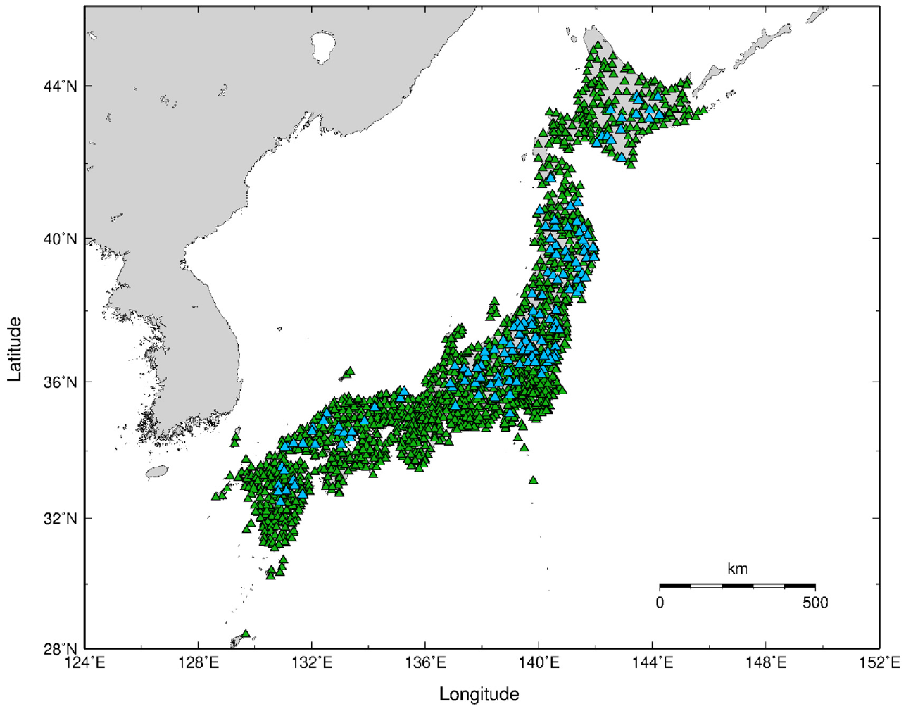
Spatial distribution of the 1725K-NET and KiK-net recording sites used in this study. Here 1580 sites (green triangles) are used for training and the remaining 145 sites (blue triangles) for testing.

From the complete data set, we arbitrarily select 145 sites for testing (Supplemental Table S1, see “Data and Resources”) and the remaining 1580 sites for training (Figure 2). The 145 testing sites are representative of the full data set in terms of spatial coverage and statistical distribution of site parameters. In the companion paper, the training sites were used to derive correction spectra for c-HVSR, whereas the testing data set was earmarked for evaluating and comparing the performance of different site-specific approaches, including c-HVSR, 1D-based GRA, and SRI methods. Likewise, in this article, we develop parametric and non-parametric site-response models on the training data and then examine and compare their effectiveness at the testing sites (Figure 3).

Table 1.

Percentage of reduction in between-site variability in site response (( $ϕ_{S 2 S}^{0} - ϕ_{S 2 S}^{m}$ )/ $ϕ_{S 2 S}^{0}$ )

f (Hz)	RF1	RF2	RF3	RF4	RF6	RF7^*	GRA (V1)	GRA (V2)^*	c-HVSR^*
0.1–3.0	16%	26%	23%	29%	36%	41%	34%	34%	30%
0.1–10.0	11%	23%	19%	26%	31%	38%	25%	31%	28%

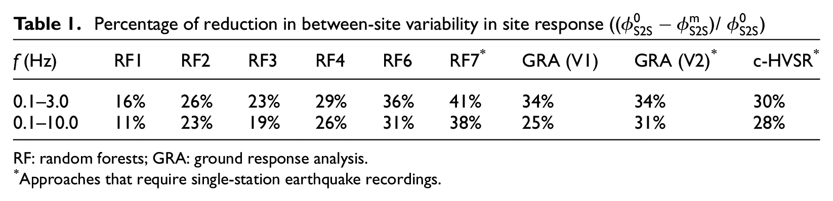
RF: random forests; GRA: ground response analysis.

Approaches that require single-station earthquake recordings.

Figure 3.

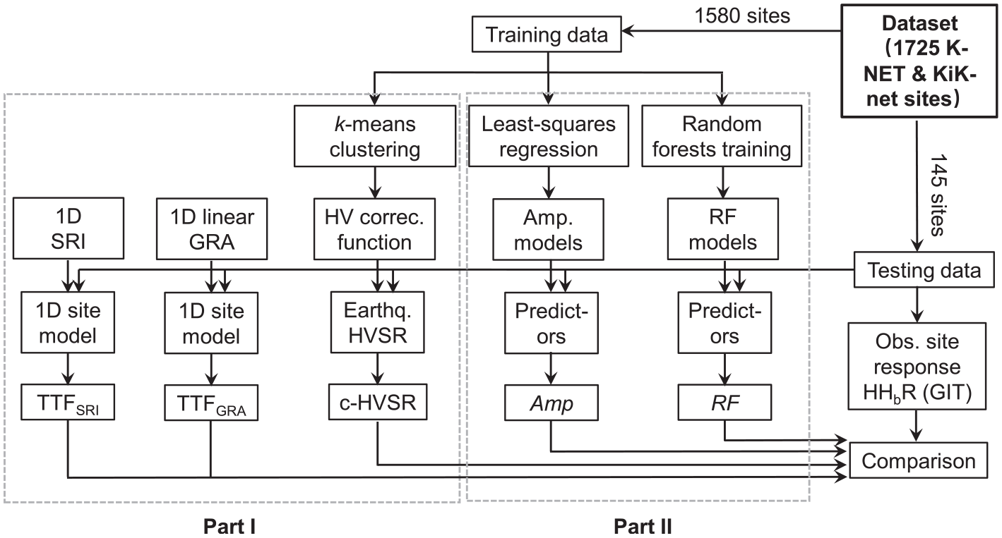
Flowchart illustrating the evaluation of different site-response estimation approaches. TTF—theoretical transfer function from either 1D ground response analysis (GRA) or the square-root-impedance (SRI, also called quarter-wavelength) method; c-HVSR—corrected HVSR; Amp—parametric site-response models by least-squares regressions; and RF—fully data-driven site-response models by random forests (a supervised ML technique) (after Zhu et al., 2021a).

Site metadata at the 1725 stations are collected from an open-source site database developed by Zhu et al. (2021c, see “Data and Resources”). Considered predictor variables include topographic roughness (Roug., the largest difference in elevation between the target pixel and the surrounding cells on a digital elevation model, DEM), geological unit (Geo.), geomorphological category (Geomorp), V_S₃₀, predominant frequency on HVSR curve (f_{P, HV} or f_p for brevity), depth to SH-wave velocity 2.5 km/s horizon from the Japan Seismic Hazard Information Station (J-SHIS) 3D velocity model (Z_2.5, Fujiwara et al., 2012), the mean eHVSR curve over multiple events (A_HV(f)), and the high-frequency decay parameter kappa (κ₀). Although some of the site information is not typically considered as site metadata, for example, A_HV(f), rather we regard them as “predictor variables” of site response in a broad sense. More information on predictors can be found in the data and companion papers (Zhu et al., 2021a, 2021c).

Model development

Site-response models are predictive models relating input information, that is, predictor variables, to output, that is, site responses at different frequencies. We develop both parametric site-response models by conventional regressions in a least-square sense, and non-parametric models by a supervised ML technique—RF. Since many prior studies in different disciplines have demonstrated the potential of ML models for improved predictive power over regression-based ones (e.g. Kong et al., 2019), herein we do not repeat the comparison between the two. Before model development, we first classify predictor variables according to their accessibility/engineering utility (Figure 4).

Figure 4.

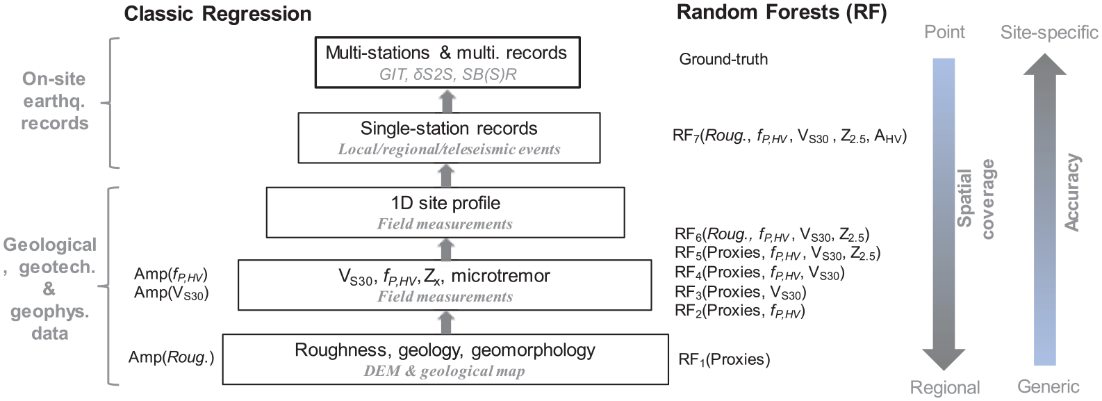
Site information pyramid according to their engineering utility. Site responses derived directly from empirical data using recording pair- or network-based techniques are used as ground truth.

Surficial proxies, including topographic roughness, geology, and geomorphology, can be readily derived from DEMs and geological maps which are available on regional or even global scales. Thus, surficial proxies are considered to be the easiest-to-obtain proxies and are often used in regional seismic hazard/risk mappings. Surficial proxies are followed by site data from on-site measurements, including V_S₃₀, f_p, Z_2.5, and microtremors (Figure 4). V_S₃₀ has been included in many seismic codes (e.g. Eurocode 8, 2004), and thus tremendous efforts have been devoted to deriving this parameter at many sites (e.g. Cultrera et al., 2021; Di Giulio et al., 2021). f_p can also be reliably obtained from mHVSR (e.g. Site EffectS assessment using AMbient Excitations (SESAME), 2004). Z_2.5 can be derived by querying regional 3D velocity models, though such velocity models only exist for a few regions. 1D site profiles can be established by invasive or non-invasive techniques.

Geological and geotechnical data, and microtremors, can be acquired in a reasonable timeframe. We thus consider them to be more accessible than single-station earthquake recordings which reply on local, regional, or teleseismic events. However, using earthquake recordings is expected to lead to a more accurate characterization of site effects. Therefore, the decision on what site data to collect for a given project needs to balance both the required level of estimation accuracy and the available resources (e.g. time and budget). To collect earthquake recordings, one may need to instrument the target sites in the planning stage of a new project. Also, we note that our grouping of site data is subjective, and the hierarchical structure of predictors (Figure 4) may vary for a specific case.

Least-squares regressions

From the training data, we develop three simple parametric models (Figure 4) by conventional least-squares regressions. Empirical data show that FAS-based site responses at different oscillator frequencies change linearly with topographic roughness (Figure 5); we thus use a linear functional form (Equation 3) to depict this relationship:

\ln Amp (Roug .) = a_{1} + a_{2} \ln (Roug .)

(3)

where a₁ and a₂ are frequency-dependent regression coefficients. Roug. represents roughness.

Figure 5.

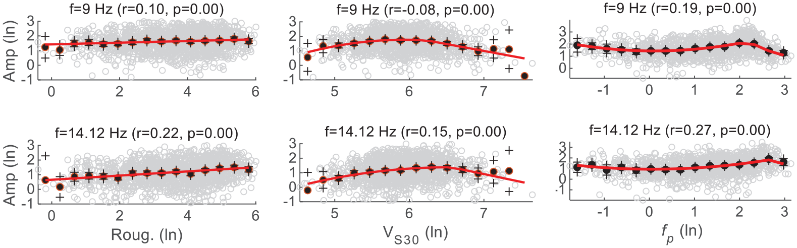
Fourier site response (ln scales) versus Roughness (left), V_S₃₀ (middle), and f_p (right) at different oscillator frequencies. In each plot, each circle corresponds to one site; black dots and plus signs represent binned means and their 95% confidence intervals of the mean estimate, respectively; and the red line denotes the prediction from regression models (Equations 3–5).

However, the trend between FAS site responses and V_S₃₀ cannot be fully described by a linear function (Figure 5), as is often adopted for PSA-based site responses. Rather, we use a piece-wise function (Equation 4) to model the complex relationship. V_c and V_L are breakpoints (velocities) that are derived from regressions as frequency-dependent parameters. There is no site response for V_S₃₀ above V_c; for V_L ≤ V_S₃₀ < V_c, site-response scales linearly with V_S₃₀; and for V_S₃₀ < V_L, there is a nonlinear relation between site response and V_S₃₀:

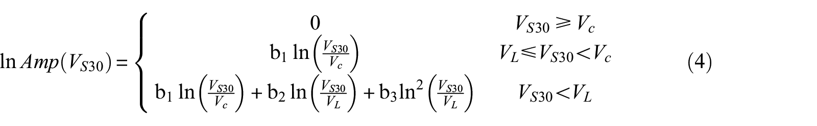
\ln Amp (V_{S 30}) = {\begin{matrix} 0 & V_{S 30} \geq V_{c} \\ b_{1} \ln (\frac{V_{S 30}}{V_{c}}) & V_{L} \leq V_{S 30} < V_{c} \\ b_{1} \ln (\frac{V_{S 30}}{V_{c}}) + b_{2} \ln (\frac{V_{S 30}}{V_{L}}) + b_{3} \ln^{2} (\frac{V_{S 30}}{V_{L}}) & V_{S 30} < V_{L} \end{matrix}

(4)

where b₁–b₃, and V_c and V_L are frequency-dependent regression coefficients.

Site responses also vary nonlinearly with f_p (Figure 5). Site response peaks at the oscillator frequency of interest (f_osc), whereas for f < f_osc and f ≥ f_osc, the trends are modeled by quadratic functions:

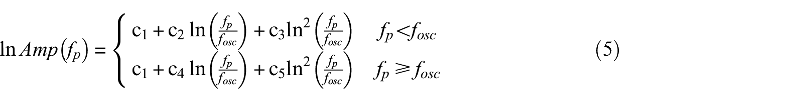
\ln Amp (f_{p}) = {\begin{matrix} c_{1} + c_{2} \ln (\frac{f_{p}}{f_{osc}}) + c_{3} \ln^{2} (\frac{f_{p}}{f_{osc}}) & f_{p} < f_{osc} \\ c_{1} + c_{4} \ln (\frac{f_{p}}{f_{osc}}) + c_{5} \ln^{2} (\frac{f_{p}}{f_{osc}}) & f_{p} \geq f_{osc} \end{matrix}

(5)

where c₁–c₅ are frequency-dependent regression coefficients. All model parameters and coefficients in Equations 3–5 are solved in regressions on the training data set and are provided as Supplemental material (see “Data and Resources”). The testing data are absent during model developments.

Random forests

In addition to conventional regressions, we use an ensemble ML approach, RF, to perform multivariate non-parametric and nonlinear regressions. Data-driven approaches do not require pre-defined functional forms and can model the complex relationships embodied in data, which is an appealing feature when it comes to multivariate regressions. RF is a supervised technique and requires hand-crafted features (explainable variables). RF is adopted mainly because RF models are transparent or explainable, as opposed to many “black box” algorithms because gaining insight is as important as achieving high prediction accuracy, if not more.

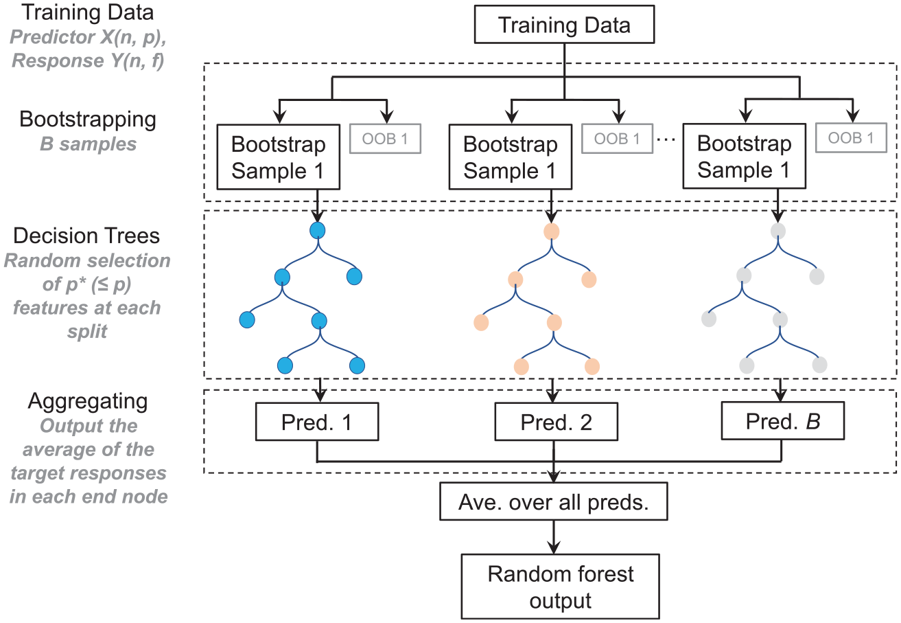
The RF training algorithm (e.g. Breiman, 2001) applies the technique of bootstrap aggregating, or bagging, to tree learners (Figure 6). Bagging generates B number of bootstrap replicas of the training data set, $X^{b}$ and $Y^{b}$ (b = 1, 2,…, B). Each bootstrap sample b is established by randomly selecting n out of n observations with replacement (one observation may appear multiple times in one bootstrap sample), and observations not selected for that bootstrapped data set (on average 37%) are placed in a separate Out-of-Bag (OOB) data set. OOB data enable users to conveniently estimate the generalization error of an RF model during its development, and it is not necessary to reserve a separate data set for validation or testing.

Figure 6.

RF regression. X and Y are column matrices that contain predictor and site-response data, respectively. Each row in X and Y corresponds to one site. Each column in X represents one predictor variable, and each column in Y corresponds to the site response at a given oscillator frequency. n, p, and f are the total numbers of sites, predictor variables, and oscillator frequencies considered in this study. B is the total number of bootstrapped samples (or trees), and p* is the number of predictor variables selected at random at each decision split. OOB is the out-of-bag data.

The training data set, consisting of predictor variables $X_{i, j}$ (i = 1, 2,…, n and $j$ = 1, 2,…, p) and site responses $Y_{i, f}$ (Figure 6), is used to develop the RF models. n is the total number of observations, that is, 1580 sites in the training data set, p is the number of predictor variables, and f represents oscillator frequency. RF models are trained for 33 logarithmically spaced oscillator frequencies. A detailed description of RF models is provided in the Supplemental material (see “Data and Resources”).

We start developing RF models using only surficial proxies and then add more predictors into the model, thus a series of RF models are trained (Figure 4). In this study, single-station earthquake recordings are simply used in the form of eHVSR, but other representations of single-station recordings can be explored in the future. Considering engineering utility, mHVSR is preferred over eHVSR, but microtremors are unavailable at most KiK-net and K-NET sites.

Model explanatory powers

Model explanatory power denotes to what degree the model explains the variability in the training data. First, we check the residuals of each model. The residuals of the RF model RF7 (Figure 7) at f = 9 and 14.12 Hz are centered at zero and have no systematic trend against their corresponding predictor variables. This is also true at the other oscillator frequencies and for other models (not shown here for brevity but provided as Supplemental material, see “Data and Resources”). These demonstrate that the trends between site responses and predictor variables in the data are successfully captured by both the regression and RF models developed here.

Figure 7.

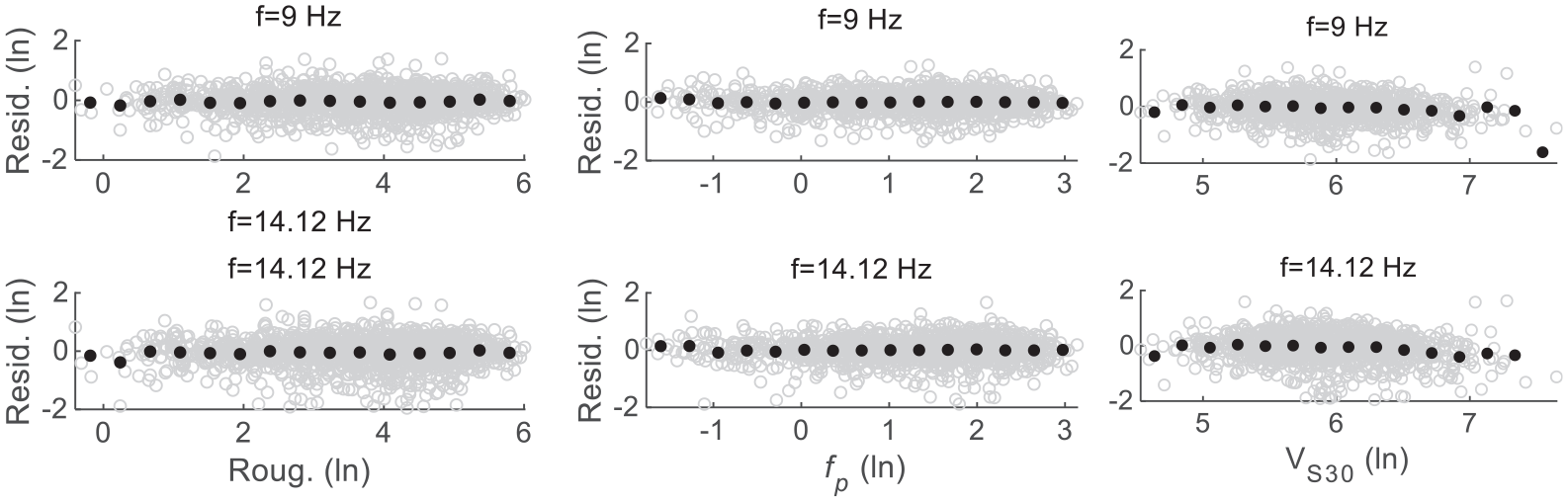
Residuals of the RF model RF7 (Figure 4) against its main predictor variables at selected frequencies. In each plot, black dots represent binned means.

Next, we assess the explanatory powers of each RF model (Figure 8) using the coefficient of determination (R²) which reflects the proportion of variance explained by each model. R² is derived using the OOB data and represents an independent evaluation of the model explanatory powers. As expected, the model RF1 using Proxies (the combination of roughness, geology, and geomorphology) is the least effective in explaining the data variance, especially at relatively high frequencies (f > ∼3.0 Hz) where less than 10% of variance is accounted for. However, RF1 can be readily applied in site-response mapping on a regional or even global scale. With the inclusion of more and more predictors from field measurements, model explanatory powers are significantly improved. RF7 is the best-performing model which accounts for as high as 70% of the variance at f = ∼0.5–1.0 Hz. However, at higher frequencies, for example, at f = 12.15 Hz, RF7 explains only 30% of the variance. Such complex site-response models as RF7 can be used in site-specific studies. Therefore, when considering site-response models, one needs to balance its spatial coverage and estimation accuracy.

Figure 8.

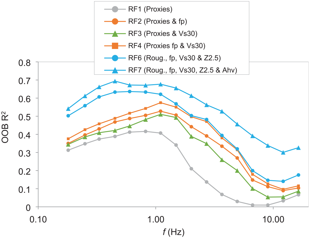
Model explanatory powers using coefficient of determination (R²). R² is estimated using the OOB data during the training of each RF model. Proxies denote a cluster of three topographic/geological features, including topographic roughness, surface geology, and geomorphology.

We then examine the relative importance of individual predictor variables in RF models, as exemplified in Figure 9 for RF7. Results for other RF models are provided as Supplemental material (see “Data and Resources”). In RF1, Proxies (roughness, geology, and geomorphology) are effective at relatively low frequencies (<∼1.0 Hz), especially roughness. This confirms previous results (e.g. Thompson and Wald, 2016; Weatherill et al., 2020) that topographic proxies reflect the deep subsurface structures. However, when Z_2.5 (inferred from the J-SHIS velocity model) is included (i.e. RF5), geology and geomorphology become insignificant. This is because, although geology, geomorphology, and Z_2.5 are all indicators of deep velocity structures, Z_2.5 is a continuous quantity, whereas geology and geomorphology are categorical variables. Thus, Z_2.5 is a significantly more effective predictor of site responses at relatively low frequencies than the latter two. For this reason, we exclude geology and geomorphology in the subsequent models, that is, RF6 and RF7 in which Z_2.5 is incorporated.

Figure 9.

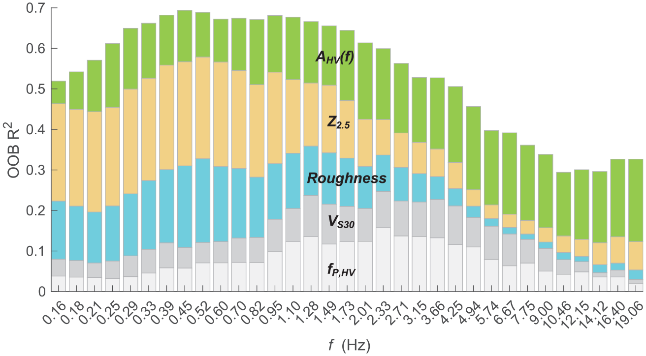
Unbiased estimates of the relative importance of predictors in the RF model RF7 using OOB data. The height of each column is scaled to represent the coefficient of determination R² as shown in Figure 8.

Both V_S₃₀ and f_p contribute to the reduction in variance in the mid-frequency range, but f_p is more effective than V_S₃₀ (Figure 9). This is consistent with many previous findings, for example, by Zhu et al. (2020b) who suggested using f_p as the primary and V_S₃₀ as the secondary predictor variable. Among all explanatory variables considered here, A_HV(f) is the only one performing well at all examined frequencies and is also the most effective at frequencies higher than 10 Hz.

Model predictive powers at the 145 testing sites

Model explanatory power only quantifies the proportion of explained variance in the training data. However, it is the predictive power of a model, namely the ability to explain the variability in unseen data, that is relevant in seismic hazard/risk analyses (e.g. Bindi, 2017). Therefore, the evaluation of predictive models should be based on data that are unseen by the models under evaluation (e.g. Mak et al., 2017). In this section, we test the regression (Amp) and RF amplification models at the 145 testing sites which are completely “hidden” from the model development (Figure 3). For illustration purposes, predictions are compared with observation at one test site FKSH05 in Figure 10, while results for all other sites are provided as Supplemental material (see “Data and Resources”).

Figure 10.

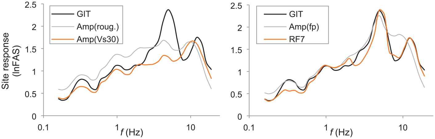
Observed (from GIT) versus predicted site responses at the test site FKSH05 using Amp(Roug.), Amp(V_S₃₀), Amp(f_p), and RF7. GIT site response is the same in both plots. lnFAS represents results based on Fourier domain in ln scales.

As shown in Figure 10, RF7 and Amp(f_p) estimates match the observation well and can capture the resonance at f = 4.9 Hz due to the inclusion of f_p in both models. In contrast, predictions from Amp(Roug.) and Amp(V_S₃₀) significantly underestimate the resonance. The distributions of residuals at the 145 testing sites (Figure 11) demonstrate that Amp(V_S₃₀), Amp(f_p), and RF7 are not biased. This is also true for Amp(Roug.) and other RF models (see “Data and Resources”).

Figure 11.

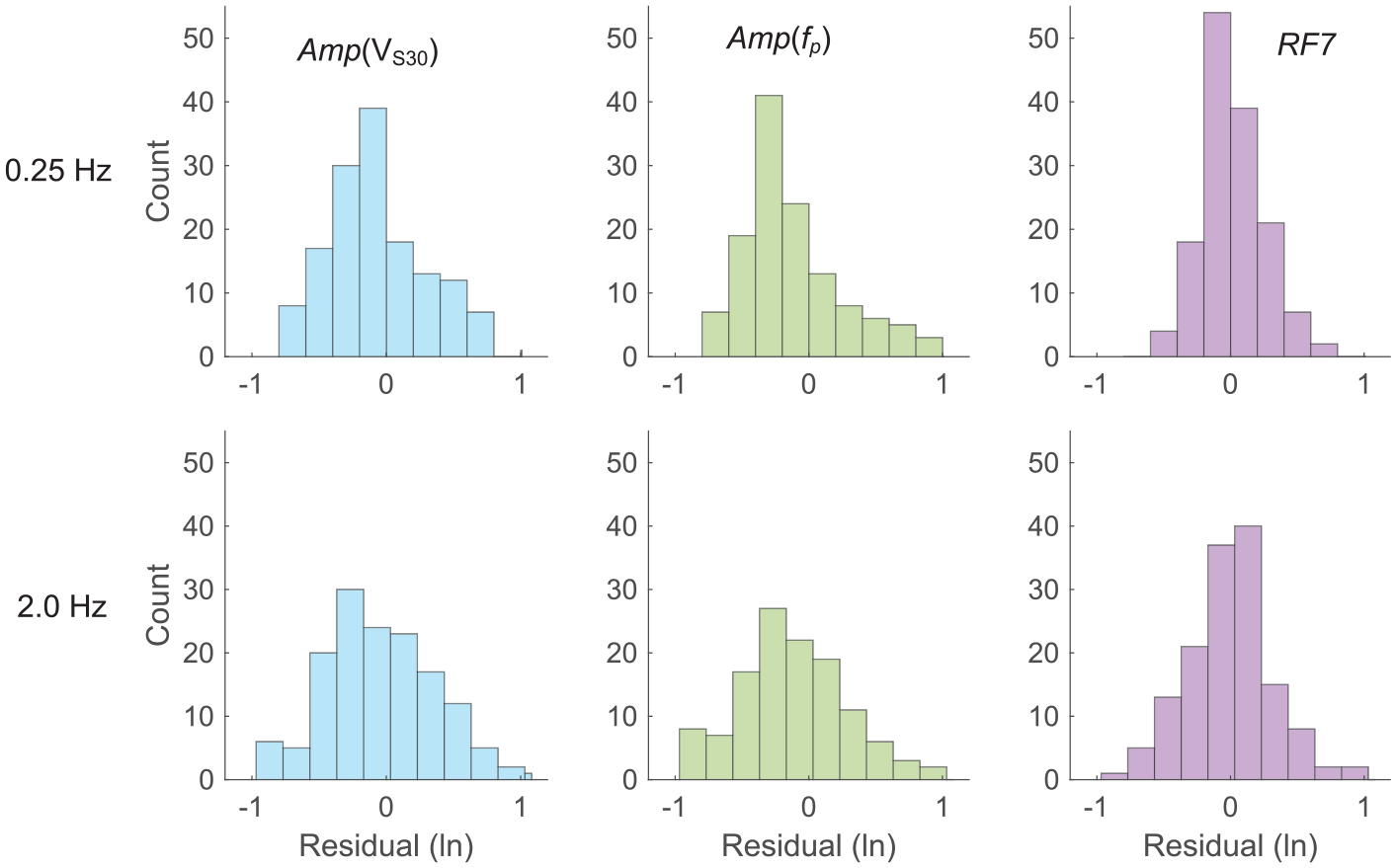
Histograms of residuals between site-response observation and predictions from the parametric models Amp(V_S₃₀), Amp(f_p), and RF model RF7 at f = 0.25 Hz (first row) and 2.0 Hz (second row) at the 145 testing sites.

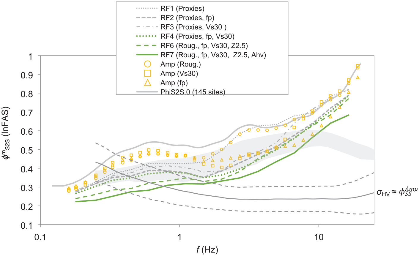
Then we assess to what extent each estimation model/approach can capture the site-specific features of site responses at the 145 testing sites as a whole (Figure 12). This is achieved using the reduction of $ϕ_{S 2 S}^{m}$ relative to $ϕ_{S 2 S}^{0}$ . $ϕ_{S 2 S}^{m}$ is the standard deviation of residuals between observed site responses and predictions from a given model/method m at the 145 sites. $ϕ_{S 2 S}^{0}$ represents the spatial variability of the full site responses at the 145 sites. Assuming the model/method m is effective, the reduction in the between-site variability, that is, $ϕ_{S 2 S}^{0} - ϕ_{S 2 S}^{m}$ , reflects the overall performance of the model/method in reproducing the observed site-specific amplification spectra.

Figure 12.

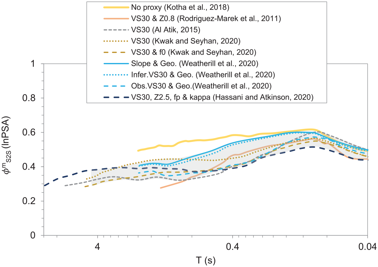
Comparison of between-site variability $ϕ_{S 2 S}^{m}$ of regression (Amp) and RF models at the 145 testing sites. Proxies include three topographic proxies: roughness, geology, and geomorphology; $ϕ_{S 2 S}^{0}$ is the variability of the full site responses at the 145 sites. Also presented is the single-station eHVSR sigma (σ_HV) which Zhu et al. (2021b) found to approximate the within-site variability in site response (i.e., $ϕ_{SS}^{Amp}$ , the standard deviation of the event-specific residual $δ Am p_{es}$ in Equation 1). Shaded zone envelopes the $ϕ_{S 2 S}^{m}$ (lnPSA) of GMM-native site-response models for Japan as shown in Figure 1.

It is worth noting the large between-site variability at frequencies higher than ∼8 Hz, which is absent in PSA-based results (shaded zone in Figure 12). This high-frequency between-site variability in the Fourier domain is consistent with other FAS-based results (e.g. Bora et al., 2019). However, PSA-based between-site variability (Figure 1) is significantly lower at f > ∼8 Hz. This is because, at high oscillator frequencies, the PSA ordinate is not directly proportional to that of the corresponding FAS at the same oscillator frequency, rather it is controlled by a wide band of FAS ordinates (e.g. Bora et al., 2016). This is consistent with the results of Bindi et al. (2017) who reported that PSA-based ground motion variation does not fully capture the high-frequency variability.

Both regression and RF models can reduce the between-site variability in site response (Figure 12). With the inclusion of more and more predictor variables in RF models, the dispersion is further lowered, which agrees with the pattern depicted in Figure 8 using OOB data during the training. For the best-performing model RF7, the between-site variability can be reduced by as much as 0.27 (ln scales) at f = ∼2.7 Hz, though the reduction at higher frequencies is less significant. In the frequency range between 0.1 and 10 Hz, on average, RF7 can lower the variability by 38% (Table 1).

Comparing ML with 1D GRA

In addition to the regression (Amp) and RF models, site responses are also estimated using GRA or SRI, and c-HVSR at the 145 testing sites. The performance of these techniques was assessed in the companion paper (Zhu et al., 2021a). GRA and SRI require 1D site models, including both SH-wave velocity (V_S) and small-strain damping (D_min) profiles for linear analyses. Zhu et al. (2021a) constructed composite profiles (referred to as “V1”) reaching seismological bedrock with V_S = 3.45 km/s. KiK-net profiles from borehole logging (referred to as “V0”) were used to fill the portion from the ground surface to borehole depth, whereas J-SHIS profiles were used for the section below. Based on V1, new velocity structures were developed by inversion from eHVSR, referred to as eHVSR-consistent structure “V2.” D_min profiles were established from V_S using the D_min–V_S relationships proposed by Campbell (2009) and J-SHIS, referred to as “D1” and “D2” models, respectively. For c-HVSR, correction spectra were established for different site categories from the training data in the companion paper.

ML versus 1D physics-based modeling

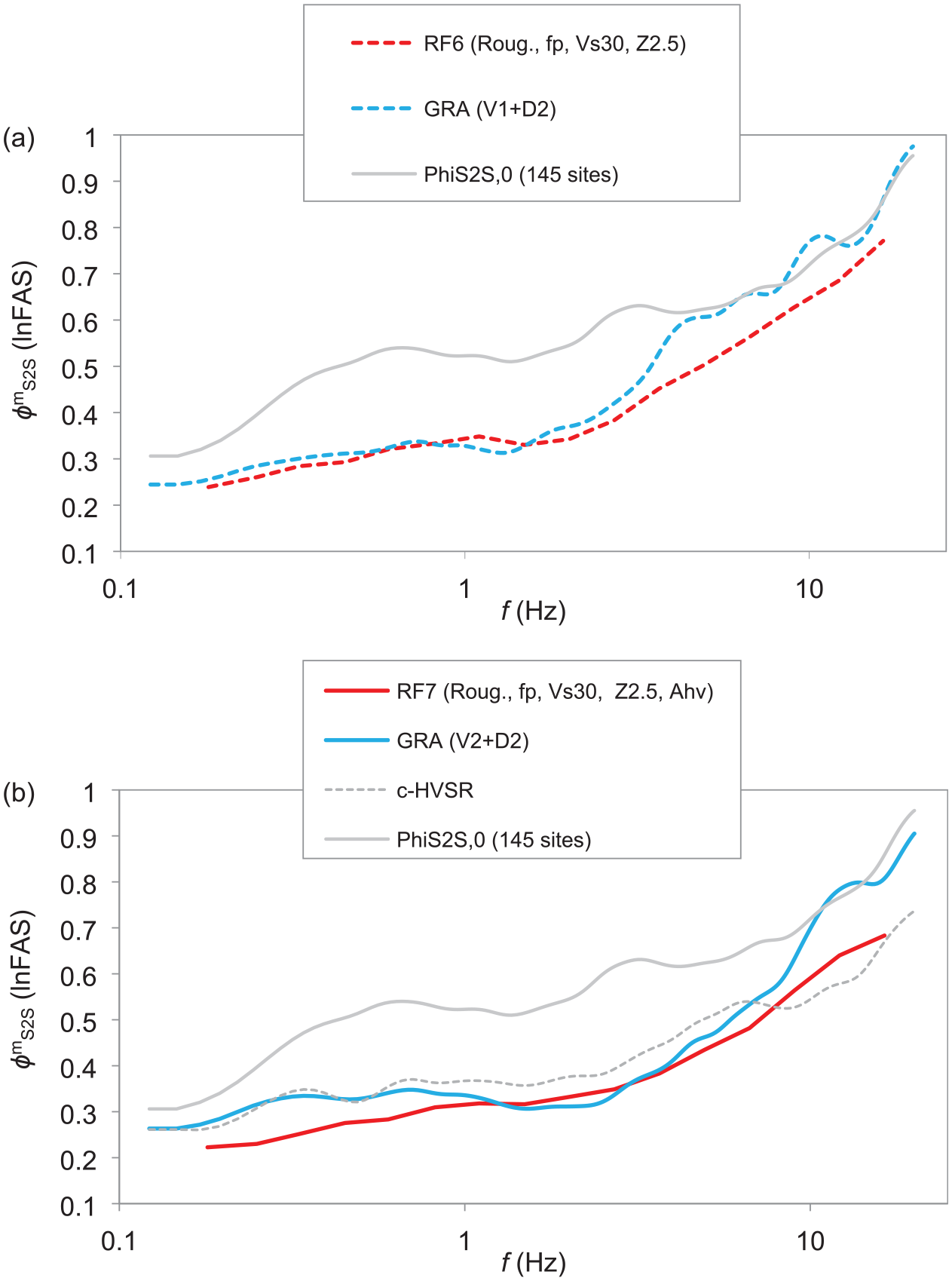
Examining the effectiveness at the testing sites as a whole, GRA using V1 performs poorly at relatively high frequencies (Figure 13a). For f < ∼3.0 Hz, GRA (V1) is effective, on average reducing between-site variability by 34% (Table 1). However, in the range ∼3.0–4.0 Hz, its effectiveness starts declining, and for f > ∼4.0 Hz, GRA (V1) leads to no reduction in dispersion. The poor performance of GRA (V1) at high frequencies is primarily due to our limited ability to precisely depict small-scale variations in V_S and site attenuation properties. In the broader frequency range of 0.1–10 Hz, GRA (V1) can only reduce the between-site variability by 25%.

Figure 13.

Comparison of $ϕ_{S 2 S}^{m}$ (lnFAS) of different estimation techniques at the 145 testing sites: (a) RF6 and GRA (V1) and (b) RF7, GRA (V2) and c-HVSR (all need single-station earthquake recordings). RF—random forest model, GRA—1D ground response analysis, and c-HVSR—empirical correction to eHVSR. V1 corresponds to the composite velocity profile (KiK-net + J-SHIS), whereas V2 represents the inverted profile from eHVSR. D2 is the generic damping model from J-SHIS. $ϕ_{S 2 S}^{0}$ (same in both plots) is the variability of the full site responses at the 145 testing sites.

RF models using a few predictor variables could capture more site-specific features of site responses than GRA using detailed 1D earth structures (V1) (Figure 13a). In the frequency range where GRA (V1) is effective, that is, 0.1–3.0 Hz (Table 1), GRA (V1) can achieve a larger margin of reduction in between-site variability (i.e. 34% on average) than RF1–4 models. However, the predictive model RF6 (Roug., f_p, V_S₃₀, Z_2.5) starts outperforming GRA (V1). In the broader frequency range of engineering interests, that is, 0.1 < f < 10.0 Hz, even the predictive model RF4 (Proxies, f_p, V_S₃₀), where Proxies contain Roug., Geo., and Geomorp., has a slightly lower dispersion than GRA (V1) (Table 1). Subsequent RF models using more predictors have much lower dispersions than GRA (V1).

Use of single-station earthquake recordings

In some site-specific applications, on-site recordings could be collected by instrumenting the target sites to record earthquakes that may be irrelevant for seismic hazard analyses, for example, very distant large events (e.g. Hollender et al., 2018). These on-site recordings may not support the application of recording pair- or network-based empirical techniques, that is, GIT, δS2S_s, and SB(S)R, due to, for instance, the lack of a proper nearby reference site or a regional network. However, they can be used on a single-station basis, for example, in GRA and RF7, to improve the site-specific characterization of site response.

Single-station recordings of weak motions can be used to calibrate the 1D velocity structures to be used in GRA. GRA using V2 profiles from inversion of eHVSR (Figure 13b) can further reduce the between-site variability at frequencies between ∼2 and ∼10 Hz in comparison with GRA (V1) (Figure 13a). This is detailed in the companion paper (Zhu et al., 2021a). In 0.1–10 Hz, GRA (V2) can lower the variability by 31%, as opposed to 25% for GRA (V1) (Table 1). This demonstrates the benefits of collecting on-site recordings.

However, even if earthquake recordings are used to constrain the 1D models for GRA, RF models still could achieve a lower between-site variability (Figure 13b). For 0.1 < f < 10 Hz, RF6, based on a few predictors (i.e. Roug., f_p, V_S₃₀, and Z_2.5), has a similar level of dispersion as GRA (V2) which needs a detailed 1D ground model and on-site recordings (Table 1). If the whole eHVSR curve is also fed into the RF model, that is, RF7, a larger reduction in the dispersion can be realized, 38% for RF7 while 31% for GRA (V2) (Table 1). This again manifests that ML (i.e. RF) is more effective than 1D physics-based modellings in using existing site information.

From using only eHVSR peak frequency to using the whole curve

If eHVSR is available, the whole curve can be used in site-response predictive models, rather than just its peak parameters. The frequency-dependent eHVSR is effective in the whole frequency range 0.1–20 Hz (Figure 12). For 0.1 < f < 10 Hz, RF7 (Roug., f_p, V_S₃₀, Z_2.5, A_HV) can lower the between-site variability by 38%, larger than 31% for RF6 (Roug., f_p, V_S₃₀, Z_2.5) using only the peak frequency (Table 1). This demonstrates the effectiveness of eHVSR as a vector-valued predictor (Figure 9).

Another way of using the whole eHVSR curve is through a simple correction, that is, the c-HVSR approach which is also quite promising (Figure 13b). c-HVSR performs better than GRA at high frequencies (>∼8.0 Hz). Although c-HVSR results have a higher dispersion than RF6 and RF7 in the frequency range 0.1–10 Hz (Table 1), c-HVSR is still appealing considering the simple input information that it requires.

We acknowledge that mHVSR maybe preferred over eHVSR considering engineering utility. mHVSR is not used in the current study because microtremors are unavailable at most KiK-net and K-NET sites. However, the performance of eHVSR shown here (e.g. Figure 9) is still useful because we assume it is an upper bound performance limit of mHVSR.

Discussion

Uncertainty/variability in site-response estimates

Regression and RF models, c-HVSR, and GRA are, in essence, conceptual/mathematical/physical representations of the natural world (i.e. the complex wave propagation within near-surface geology). These approximations have two sources of uncertainties (Abrahamson et al., 1990): modeling and parametric (Table 2). For the estimation of site responses, modeling uncertainty arises from the simplifications/assumptions/approximations made to the natural world, while parametric uncertainty represents the uncertainty in accurately defining input parameters and model coefficients (Table 2). Both parametric and modeling uncertainties have epistemic and aleatory components (Toro et al., 1997).

Table 2.

Uncertainty/variability in site-response estimates

	Epistemic (reducible)	Aleatory (irreducible but quantifiable)
Modeling	Uncertainty in the median prediction of site response due to the simplifications or assumptions made in regression models (e.g. the “averaging” effects and imperfect functional forms) and 1D GRA (e.g. neglection of basin effects).	Unexplained scatter due to the inherent randomness in the physical processes that cannot be reduced within empirical regression models and 1D GRA, for example, the azimuth and incident angle dependence of site response.
Parametric	Uncertainty in the median values of input parameters (i.e. explanatory variables and coefficients in regression models, and V_s and D_min profiles, MRD curves, and SH strength for GRA) due to, for example, the limitations of current site-characterization techniques.	Spatiotemporal variation in the numerical values of input parameters, for example, time-dependent variation in soil properties due to nonlinearity following large earthquakes or meteorological factors (e.g. rainfall, freezing, and thawing), and the laterally variable nature of soil properties within the site scale.

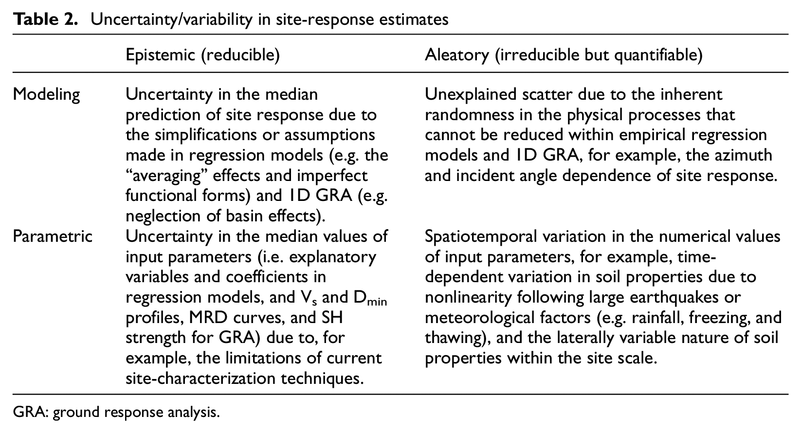
GRA: ground response analysis.

Aleatory variability (Table 2) is the inherent or natural randomness of site response, for example, the variation from event to event at a single site, and it is irreducible for a model/method m but quantifiable through repeated observations at the same site. However, epistemic uncertainty arises because our site responses are predicted using models/simplified approaches (mathematical and conceptual constructs of reality), and thus it comes with uncertainty due to our lack of data or knowledge, or simplifications/assumptions concerning the validity of the models/approaches (e.g. GRA assumes vertically propagating SH-waves through 1D soil columns, that is, the 1DSH assumptions) or errors in the numerical values of their input parameters (e.g. median Vs profiles in GRA). However, epistemic uncertainty is, in principle, reducible through further research and gathering more and better data, for example, using aggravation factor (e.g. Chávez-García and Faccioli, 2000) to adjust GRA results to account for basin effects. As pointed out by many (e.g. Toro et al., 1997), the distinctions of modeling versus parametric, and epistemic versus aleatory (Table 2) are model/method-dependent. Their partitions are conceptually clear but are often difficult in reality. However, such distinctions are necessary for their subsequent proper treatments, rather than for philosophical reasons.

In this study, $ϕ_{S 2 S}^{m}$ (Figures 12 and 13) is derived by comparing predictions to observations and thus reflects both parametric and modeling uncertainties for a given model/approach m (Table 3). In addition, the target in this study is the average site response over many earthquakes (at least five) at each site (Equation 2). This average site response is a deterministic quantity at a given site, and thus the term $ϕ_{S 2 S}^{m}$ is considered to only reflect the epistemic component and can be reduced to zero in theory. We stress that $ϕ_{S 2 S}^{GRA}$ reflects the overall level of epistemic uncertainty at the sample sites (the 145 testing sites) but does not represent the epistemic uncertainty of GRA at any specific site. Epistemic (parametric and modeling) uncertainties in GRA predictions vary from site to site and should be quantified on a site-specific basis. For instance, a site near the basin edge is expected to have a higher modeling error than a site in the central region of a large basin.

Table 3.

Site effect prediction and its associated uncertainty and variability

Method	Input	Mean predication (µ)				Epistemicuncertainty(this study)	Aleatoryvariability(Zhu et al., 2021b)
Method	Input	Impedance and resonance	Nonlineareffects	Basineffects	Topographiceffects	Epistemicuncertainty(this study)	Aleatoryvariability(Zhu et al., 2021b)
GRA	1D site model	✓	--	X	X	ϕ _S2S ^GRA	ϕ _SS ^Amp
RF6	Roug., f_p,V_S₃₀, Z_2.5	✓	--	✓	✓	ϕ _S2S ^RF6

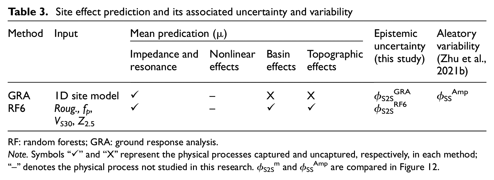
RF: random forests; GRA: ground response analysis.

Note. Symbols “✓” and “X” represent the physical processes captured and uncaptured, respectively, in each method; “--” denotes the physical process not studied in this research. ϕ_S2S^m and ϕ_SS^Amp are compared in Figure 12.

Aleatory variability in site response (i.e. $ϕ_{SS}^{Amp}$ , the standard deviation of the event-specific residual $δ Am p_{es}$ in Equation 1) is quantified by Zhu et al. (2021b) who found that it can be approximated by the between-event variability in eHVSR, that is, σ_HV, as displayed in Figure 12. For f > ∼1.0 Hz, between-event (aleatory) variability is relatively stable across frequency, centering at 0.23–0.28 (ln scales, a linear scale factor of 1.26–1.32), which is much lower than the between-site variability (Figure 12). This justifies that priority shall be given to better model the site-specific (mean) site response over the event-specific site effects. Since in this study, we use the average site response at each site as the target, rather than the event-specific site response, aleatory variability remains the same for all the models/approaches examined here (Table 3). Note that some parts of aleatory variability in site response can potentially be reduced, for example, capturing the azimuthal dependence in a 3D modeling framework (including fault) in which these aleatory components become epistemic.

Why could ML outperform 1D physics-based modeling?

ML (RF) models using a few explanatory variables could capture more site-specific frequency-dependent features of site responses than physics-based simulations (GRA) using detailed 1D earth structures (V1) (Table 1). However, one shall not be surprised by this finding given that ML techniques have been shown to outperform physics-based modellings in many other disciplines, for example, material science, applied physics, and computational biology (e.g. Alipanahi et al., 2015). This finding in the domain of site-response estimation may be disappointing for many geotechnical earthquake engineers because GRA is often regarded as a site-specific approach. In the following, we will explain why RF models could outperform 1D physics-based modeling.

The parametric uncertainty in GRA results mainly comes from the imperfect representation of the true but unknown 1D site models (e.g. V_S and D_min for linear analyses). Detailed 1D models used in GRA inherently come with a high level of parametric uncertainty, especially in the small-scale variations in material properties. Although the 1D models at the testing sites (KiK-net) are obtained from invasive approaches which are often considered as the “ground truth,” the InterPACIFIC blind tests (Garofalo et al., 2016a) clearly show that estimated V_S profiles at a specific site from independent teams using invasive approaches (i.e. cross-hole, downhole, PS suspension logging, and seismic dilatometer test) have a similar level of uncertainty to those using non-invasive techniques, that is, surface and body wave methods. Besides, many KiK-net stations are installed in mountainous regions or margins of sedimentary basins. Such complex geological conditions are unfavorable for invasive methods (Garofalo et al., 2016a, 2016b), especially the shallow portion within 3–4 m from the surface, further inflating the parametric uncertainty in GRA predictions.

In comparison, for regression and RF models, parametric uncertainty arises from the uncertainty in the numerical values of predictor variables and model coefficients (Table 2). However, predictor variables in these models are relatively simple and can be measured or derived with a high accuracy. Furthermore, using a large data set, coefficients of these models can be well constrained with a low margin of error. Thus, we assume that GRA predictions have a higher level of parametric uncertainty than those from regression and RF models developed in this study.

The modeling uncertainty for regression and RF models is mainly because of the underlying assumption that sites in the same class defined by predictor variables would behave in the same way during earthquakes. Thus, regression models, especially those embedded in GMMs (e.g. Douglas and Edwards, 2016), only give estimates in an average sense, resulting in a large modeling error. However, with the use of multiple predictor variables, the modeling error can be significantly lowered. For instance, with the simultaneous use of roughness, f_p, V_S₃₀, and Z_2.5 in RF6, a site is “vividly” depicted in different dimensions (both lateral and horizontal) and different spatial scales. Besides, these predictors have a physical basis (Table 3). For instance, roughness is considered to be correlated with topographic effects (e.g. Rai et al., 2017), f_p is an indicator of resonance (e.g. Zhu et al., 2020b), and Z_2.5 is arguably related to deep basin effects (e.g. Campbell and Bozorgnia, 2014). As a consequence, RF6 predictions are less generic and can satisfactorily capture many site-specific physical features in site responses at individual sites, thus leading to a reduced modeling error.

In contrast, the modeling error in GRA predictions is primarily due to the underlying 1DSH assumptions. These assumptions are very likely to be violated, to different extents, at many actual sites, especially those having prominent 2D or 3D features (e.g. Pilz and Cotton, 2019) and those prone to surface waves (e.g. Furumura, 2014). In comparison, empirical predictive models are developed directly from data which are a mishmash of sophisticated site effects, for example, basin effects, topographic effects, and surface wave incidence. Thus, these complex site effects, being neglected in 1D GRA, are partially accounted for in empirical models (Table 3).

What is a site-specific approach? A unified view

The finding that the between-site variability of GRA ( $ϕ_{S 2 S}^{m}$ in Figure 13) remains large in a wide frequency range prompts us to rethink of the definition of a “site-specific” approach or the single-station sigma in probabilistic seismic hazard analysis (PSHA; Anderson and Brune, 1999). Under the ergodic assumption, the total variability $σ$ in ground motion prediction from a GMM can be expressed as:

σ = \sqrt{τ^{2} + {ϕ_{S 2 S}^{m}}^{2} + ϕ_{P 2 P}^{2} + {ϕ_{SS}^{Amp}}^{2}}

(6)

where $τ$ denotes the between-event standard deviation which represents the earthquake-to-earthquake variability not captured by the inclusion of magnitude, style of faulting, and source depth in the GMM; $ϕ_{S 2 S}^{m}$ represents site-to-site variability not captured by the site-response model m; $ϕ_{P 2 P}$ is the path-to-path variability not captured by the use of a simple distance metric; and $ϕ_{SS}^{Amp}$ describes the variability of the remaining residual which is considered to be dominated by the event-specific site effects. Often $ϕ_{P 2 P}$ is merged with $ϕ_{SS}^{Amp}$ as the event-corrected single-station standard deviation $ϕ_{ss}$ .

In PSHA, if sufficient earthquake recordings are available at the site of interest, site responses can be quantified using recording pair- or network-based techniques, that is, GIT, δS2Ss, or S(B)SR with a negligible epistemic uncertainty or standard error (e.g. Faccioli et al., 2015). Results from these techniques can capture the true but often unknown site responses at individual sites, and their corresponding $ϕ_{S 2 S}^{m}$ has no or an insignificant impact on the total sigma $σ$ . Then Equation 6 can be naturally transitioned into a single-station sigma:

σ_{ss} = \sqrt{τ^{2} + ϕ_{P 2 P}^{2} + {ϕ_{SS}^{Amp}}^{2}}

(7)

Therefore, we consider these techniques having a low $ϕ_{S 2 S}^{m}$ (∼0.2–0.3 in ln scales though it can be zero in theory) as “site-specific” approaches. However, implementing these recording pair- or network-based techniques remains challenging in many forward applications due to, for example, the lack of a proper nearby reference site or a regional network. Thus, various estimation techniques, including 1D GRA and SRI, c-HVSR, and regression and RF models, have to be adopted. At any specific sites, predictions from these estimation techniques have varying levels of over- or underestimation bias, namely epistemic (parametric and modeling, Table 2) uncertainty as represented by $ϕ_{S 2 S}^{m}$ in an average sense over many sample sites (Figures 12 and 13). Thus, their predictions are only “pseudo-site-specific,” falling between generic (global average site response) and site-specific on a continuous scale (Figure 14). To what extent these estimates are site-specific is primarily contingent on how accurately and uniquely different aspects of a site can be depicted in each method, for example, surface and subsurface material properties and their lateral and stratigraphic configurations in different spatial scales.

Figure 14.

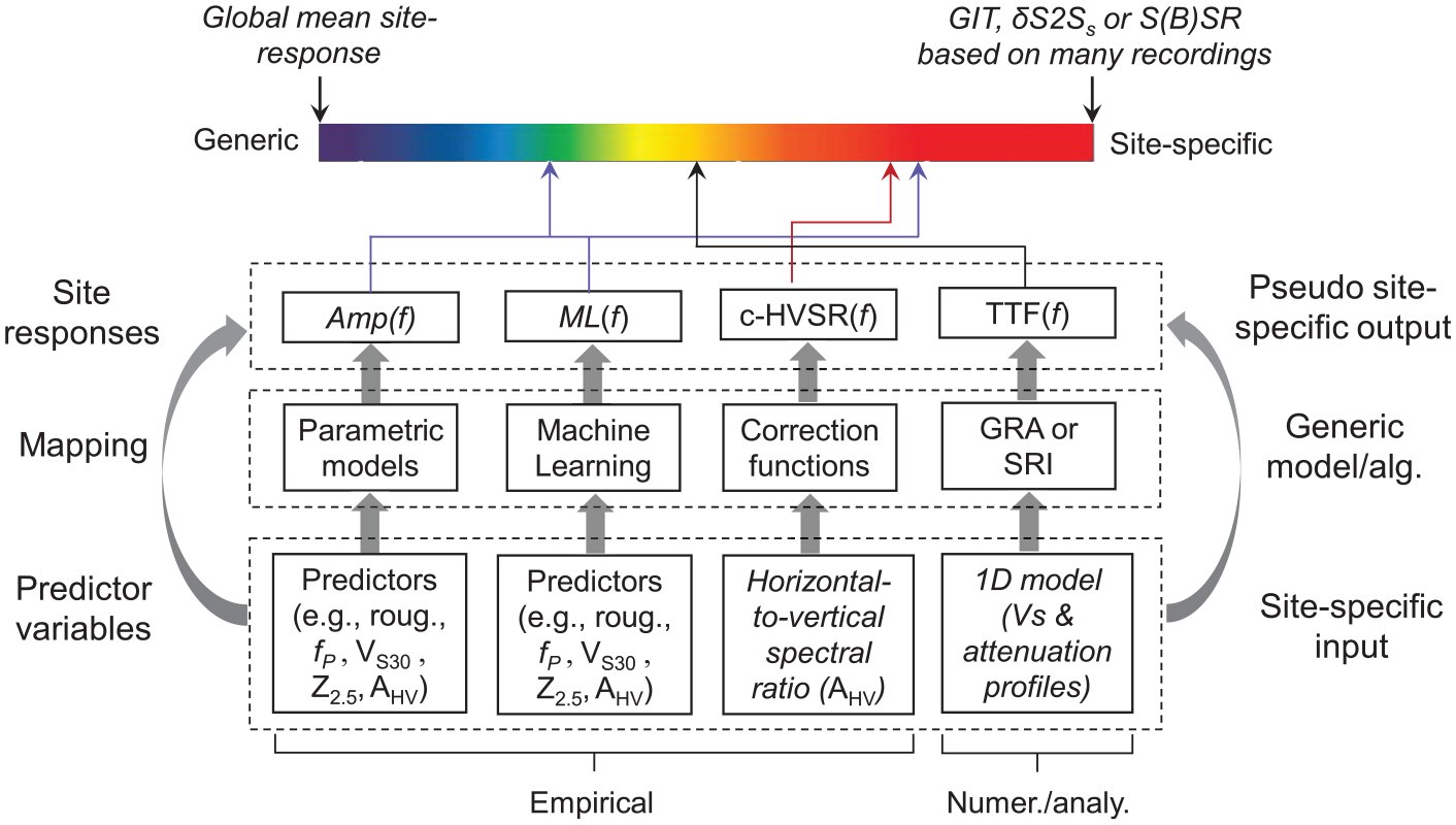
A unified view on site-response estimates from different approaches. Amp and ML—classic regression and ML models, respectively; c-HVSR—empirical correction to eHVSR; and TTF—theoretical transfer function from either 1D ground response analysis (GRA) or the square-root-impedance (SRI, also called quarter-wavelength) method.

In site-specific PSHA, 1D GRA is also regarded as a “site-specific” approach in which the single-station sigma is invoked (Equation 7). Then, the epistemic uncertainty in the mean estimate from GRA is quantified by varying input parameters (Electrical Power Research Institute (EPRI), 2012). However, this uncertainty quantification can only capture the parametric component while the modeling component is ignored (Table 2), resulting in a potential underestimation of the epistemic uncertainty in GRA results at sites where 1DSH assumptions do not hold. Unless the GRA modeling uncertainty can also be quantified on a site-specific basis, GRA prediction cannot be treated as “site-specific” as results from recordings (Figure 14).

Among the methods evaluated here, the ML models RF6 and RF7 give more “site-specific” estimation than 1D GRA (Figure 14). Considering that more complex site effects can be readily accommodated in the ML modeling framework, the fully data-driven approach could potentially be an alternative to physics-based simulations. More accurate amplification estimation improves the accuracy and reliability of hazard estimates from PSHA, especially at long return periods (e.g. Kotha et al., 2017; Stewart et al., 2017).

Possible effectiveness of RF models in other regions

Even though RF6 and RF7 outperform 1D GRA in the predictive power at the 145 KiK-net sites in this study, we note that they are trained on 1580 sites all located in Japan. One of the key advantages of 1D GRA is that it can be applied at any site characterized by a velocity profile and without referring to the previous observation data. This invites the following question: how would RF models being trained on Japanese data perform in other regions (e.g. Italy and California) in comparison with 1D GRA? This cross-domain evaluation (e.g. Münchmeyer et al., 2022) is particularly relevant for data-poor regions where we cannot afford to train a region-specific ML model, for example, Northern Europe. However, we will address this question in future studies.

There are a few hurdles in assessing the cross-domain performance of ML amplification models. For instance, the labels (observed amplifications in this case), required for supervised ML, are not created homogeneously across regions. To be specific, amplification data in Japan have a different reference condition from that in Italy. Thus, data fusion is needed and is nontrivial. Among the techniques worth exploring in cross-domain applications, one is to deploy the ML model trained for Japan via transfer learning (e.g. Pan and Yang, 2010) to target regions with fewer data. Another is to develop physics-informed ML models which are less data-hungry and more extrapolatable than purely data-driven deep learning models (e.g. Reichstein et al., 2019).

Testing the cross-domain performance of ML amplification models is beyond the scope of the article. It is, however, foreseen that the choice of the most appropriate method to predict amplification at target sites may depend on the geophysical environment and the amount of available information. Nevertheless, we have shown here the advantages of ML techniques (i.e. RF) over the 1D-based physical modeling in tackling complex site effects (e.g. surface and subsurface topographic effects).

In this study, we only employ an ML algorithm that relies on hand-crafted features (e.g. eHVSR in RF7 as the representation of single-station recordings). Using engineered features can be seen as both an advantage (e.g. domain-knowledge-guided) and a disadvantage (e.g. possibly non-optimal). For example, eHVSR in RF7 might not be the optimal representation of earthquake recordings whenever available, rather RF7 is to be re-trained with the HVSR of microtremors in the future. Nevertheless, many deep learning algorithms allow for the automatic extraction of useful information from “raw” input data and is yet to be explored here. Nonlinear site response also needs to be considered in the future. Hence, it warrants further exploration of other ML algorithms in amplification prediction, not just about improving its accuracy but also about addressing its challenges and gaining new insights into site effects.

Conclusion

To address the question of how well we can predict site-specific site responses (average over many earthquakes), we tested and compared the effectiveness of different estimation techniques using a unique benchmark data set. The benchmark data set consists of detailed site metadata and absolute Fourier outcrop linear site responses based on observations at 1725 K-NET and KiK-net sites. Evaluated approaches include 1D GRA, the SRI method (also called the QWL approach), empirical correction to the horizontal-to-vertical spectral ratio (eHVSR) of earthquakes (c-HVSR), and classic regression and RF (a supervised ML technique) site-response models. Correction spectra for c-HVSR, regression, and RF models were developed on a training data set (1580 sites). The performance of each technique is then assessed at 145 independent testing sites using the standard deviation of residuals between observations and predictions, that is, between-site (site-to-site or inter-site) variability $ϕ_{S 2 S}$ . Results on GRA, SRI, and c-HVSR were presented in a companion paper (Zhu et al., 2021a). In this study, we focus on the evaluation of classic regression and RF site-response models, and their comparison with GRA.

Our results show that ML-based model using a few predictor variables (i.e. Roug., f_p, V_S₃₀, and Z_2.5) could achieve a lower $ϕ_{S 2 S}$ than the physics-based modeling (i.e. GRA) using detailed 1D site models. This implies that ML can be more effective in using existing site information than 1D GRA which is inflicted by a high level of parametric and modeling uncertainties. In addition, we demonstrate the benefits of collecting single-station weak-motion recordings in site-specific applications, which is particularly pertinent for cases where implementing recording pair- or network-based empirical techniques remains a “luxury.” Future endeavors could further explore the modeling of complex site effects, including nonlinearity, using larger data sets and more powerful ML algorithms and address unanswered questions, for example, transferability in cross-domain applications.

Research Data

sj-xlsx-1-eqs-10.1177_87552930221116399 – for How well can we predict earthquake site response so far? Machine learning vs physics-based modeling

sj-xlsx-1-eqs-10.1177_87552930221116399 for How well can we predict earthquake site response so far? Machine learning vs physics-based modeling by Chuanbin Zhu, Fabrice Cotton, Hiroshi Kawase and Kenichi Nakano in Earthquake Spectra

This article is distributed under the terms of the Creative Commons Attribution 4.0 License (http://www.creativecommons.org/licenses/by/4.0/) which permits any use, reproduction and distribution of the work without further permission provided the original work is attributed as specified on the SAGE and Open Access pages (https://us.sagepub.com/en-us/nam/open-access-at-sage).

Research Data

sj-zip-2-eqs-10.1177_87552930221116399 – for How well can we predict earthquake site response so far? Machine learning vs physics-based modeling

sj-zip-2-eqs-10.1177_87552930221116399 for How well can we predict earthquake site response so far? Machine learning vs physics-based modeling by Chuanbin Zhu, Fabrice Cotton, Hiroshi Kawase and Kenichi Nakano in Earthquake Spectra

Supplemental Material

sj-pdf-3-eqs-10.1177_87552930221116399 – Supplemental material for How well can we predict earthquake site response so far? Machine learning vs physics-based modeling

Supplemental material, sj-pdf-3-eqs-10.1177_87552930221116399 for How well can we predict earthquake site response so far? Machine learning vs physics-based modeling by Chuanbin Zhu, Fabrice Cotton, Hiroshi Kawase and Kenichi Nakano in Earthquake Spectra

Footnotes

Acknowledgements

This work is partially supported by the project “DARE: Dense ARray for seismic site effect Estimation” funded by the French National Research Agency (Grant # ANR19-CE31-0029) and the Deutsche Forschungsgemeinschaft (DFG, German Research Foundation, project number 431362334). The authors thank the National Research Institute for Earth Science and Disaster Prevention (NIED), Japan for making the strong-motion and PS logging data available. They also thank Dr Sean K. Ahdi and two anonymous reviewers who provided very constructive feedback on this work.

Data and resources

Site parameters used in this study are obtained from an open-source site database (https://doi.org/10.5880/GFZ.2.1.2020.006). Seismograms and KiK-net borehole logging data (V0 profiles) were downloaded from http://www.kyoshin.bosai.go.jp (profiles were accessed on February 05, 2018). J-SHIS is an integrated online platform developed by the National Research Institute for Earth Science and Disaster Prevention (NIED) for the Probabilistic Seismic Hazard Maps for Japan and various underlying data (https://www.j-shis.bosai.go.jp/map/JSHIS2/download.html?lang = en). The software Strata (Kottke et al., 2013) is used for GRA. MATLAB is used to carry out least-squares and RF regressions. Supplemental material contains a table (), a word document, and a zip file. Supplemental Table S1 lists the 145 testing sites and their metadata. The word document includes detailed description of RF model training, regression coefficients of parametric models, residual plots for all models, and predictor relative importance for RF models. The “Testing.zip” contains plots of comparison between observation and model prediction at the 145 testing sites.

Declaration of conflicting interests

The author(s) declared no potential conflicts of interest with respect to the research, authorship, and/or publication of this article.

Funding

The author(s) received no financial support for the research, authorship, and/or publication of this article.

Supplemental material

Supplemental material for this article is available online.

References

Abrahamson

Somerville

Cornell

(1990) Uncertainty in numerical strong motion predictions. In: Proceedings of the 4th US national conference on earthquake engineering, Palm Springs, CA, 20–24 May, vol. 1, pp. 407–416. El Cerrito, CA: Earthquake Engineering Research Institute (EERI).

Aki

Richards

(1980) Quantitative Seismology: Theory and Methods, vols I and II. San Francisco, CA: W. H. Freeman and Company.

Al Atik

(2015) NGA-East: Ground-motion standard deviation models for Central and Eastern North America. PEER report no. 2015/09. Berkeley, CA: University of California, Berkeley. Published on June 1, 2015.

Alipanahi

Delong

Weirauch

Frey

(2015) Predicting the sequence specificities of DNA- and RNA-binding proteins by deep learning. Nature Biotechnology 33: 831–838.

Anderson

Brune

(1999) Probabilistic seismic hazard analysis without the ergodic assumption. Seismological Research Letters 70(1): 19–28.

Andrews

(1986) Objective determination of source parameters and similarity of earthquakes of different size. In: Das

Boatwright

Scholz

(eds) Earthquake Source Mechanics. Washington, DC: American Geophysical Union, pp. 259–268.

Bard

(2021) Physics-based site-amplification prediction equations: A dream at reach? In: Proceedings of the 6th IASPEI/IAEE international symposium: Effects of surface geology on seismic motion, Kyoto, Japan, 20 August.

Bergamo

Hammer

Fäh

(2021) On the relation between empirical amplification and proxies measured at Swiss and Japanese stations: Systematic regression analysis and neural network prediction of amplification. Bulletin of the Seismological Society of America 111: 101–120.

Bindi

(2017) The predictive power of ground-motion prediction equations. Bulletin of the Seismological Society of America 107: 1005–1011.

10.

Bindi

Spallarossa

Pacor

(2017) Between-event and between-station variability observed in the Fourier and response spectra domains: Comparison with seismological models. Geophysical Journal International 210: 1092–1104.

11.

Bora

Scherbaum

Kuehn

Stafford

(2016) On the relationship between Fourier and response spectra: Implications for the adjustment of empirical ground-motion prediction equations (GMPEs). Bulletin of the Seismological Society of America 106: 1235–1253.

12.

Borcherdt

(1970) Effects of local geology on ground motion near San Francisco Bay. Bulletin of the Seismological Society of America 60: 29–61.

13.

Borcherdt

(1994) Estimates of site-dependent response spectra for design (methodology and justification). Earthquake Spectra 10: 617–653.

14.

Breiman

(2001) Random forests. Machine Learning 45: 5–32.

15.

Campbell

(2009) Estimates of shear-wave Q and k0 for unconsolidated and semiconsolidated sediments in Eastern North America. Bulletin of the Seismological Society of America 99: 2365–2392.

16.

Campbell

Bozorgnia

(2014) NGA-West2 ground motion model for the average horizontal components of PGA, PGV, and 5% damped linear acceleration response spectra. Earthquake Spectra 30: 1087–1115.

17.

Chávez-García

Faccioli

(2000) Complex site effects and building codes: Making the leap. Journal of Seismology 4: 23–40.

18.

Cultrera

Cornou

Di Giulio

Bard

(2021) Indicators for site characterization at seismic station: Recommendation from a dedicated survey. Bulletin of Earthquake Engineering 19: 4171–4195.

19.

Derras

Bard

Cotton

(2017) VS30, slope, H800 and f0: Performance of various site-condition proxies in reducing ground-motion aleatory variability and predicting nonlinear site response. Earth Planets and Space 69: 133.

20.

Di Giulio

Cultrera

Cornou

Bard

Al Tfaily

(2021) Quality assessment for site characterization at seismic stations. Bulletin of Earthquake Engineering 19: 4643–4691.

21.

Douglas

Edwards

(2016) Recent and future developments in earthquake ground motion estimation. Earth-Science Reviews 160: 203–219.

22.

Electrical Power Research Institute (EPRI) (2012) Seismic evaluation guidance: Screening, prioritization and implementation details (SPID) for the resolution of Fukushima near-term task force recommendation 2.1: Seismic. Report no. 1025287, November. Palo Alto, CA: EPRI. November 2012.

23.

Eurocode 8 (2004) Design of Structures for Earthquake Resistance, Part 1: General Rules, Seismic Actions and Rules for Buildings (EN 1998-1). Brussels: European Committee for Standardization (CEN).

24.

Faccioli

Paolucci

Vanini

(2015) Evaluation of probabilistic site-specific seismic-hazard methods and associated uncertainties, with applications in the Po Plain, Northern Italy. Bulletin of the Seismological Society of America 105: 2787–2807.

25.

Fujiwara

Kawai

Aoi

Morikawa

Senna

Azuma

Ooi

Hao

Hasegawa

Maeda

Iwaki

Wakamatsu

Imoto

Okumura

Matsuyama

Narita

(2012) Some improvements of seismic hazard assessment based on the 2011 Tohoku earthquake. Technical Note of the National Research Institute for Earth Science and Disaster Prevention 379. Available at: https://scholar.google.com/citations?view_op=view_citation&hl=en&user=0J4f22YAAAAJ&citation_for_view=0J4f22YAAAAJ:M3ejUd6NZC8C

26.

Furumura

(2014) Radiation and generation of short-and long-period ground motions from the 2011 Off Tohoku, Japan, Mw9.0 earthquake. Journal of Disaster Research 9: 281–293.

27.

Garofalo

Foti

Hollender

Bard

Cornou

Cox

Dechamp

Ohrnberger

Perron

Sicilia

Teague

Vergniault

(2016a) InterPACIFIC Project: Comparison of Invasive and non-invasive methods for seismic site characterization. Part II: Inter-comparison between surface-wave and borehole methods. Soil Dynamics and Earthquake Engineering 82: 241–254.

28.

Garofalo

Foti

Hollender

Bard

Cornou

Cox

Ohrnberger

Sicilia

Asten

Di Giulio

Forbriger

Guillier

Hayashi

Martin

Matsushima

Mercerat

Poggi

Yamanaka

(2016b) InterPACIFIC Project: Comparison of invasive and non-invasive methods for seismic site characterization. Part I: Intra-comparison of surface wave methods. Soil Dynamics and Earthquake Engineering 82: 222–240.

29.

Hassani

Atkinson

(2020) Equivalent point-source ground-motion model for subduction earthquakes in Japan. Bulletin of the Seismological Society of America 111: 951–974.

30.

Hollender

Maufroy

Bard

Ameri

Perron

(2018) Are we ready to perform fully site-specific seismic hazard studies in low-to-moderate seismicity areas? In: Proceedings of the 16th European conference on earthquake engineering, Thessaloniki, 18–21 June.

31.

Ito

Nakano

Nagashima

Kawase

(2020) A method to directly estimate S-wave site amplification factor from horizontal-to-vertical spectral ratio of earthquakes (eHVSRs). Bulletin of the Seismological Society of America 110: 2892–2911.

32.

Joyner

Warrick

Fumal

(1981) The effect of quaternary alluvium on strong ground motion in the Coyote Lake, California, earthquake of 1979. Bulletin of the Seismological Society of America 71: 1333–1349.

33.

Kawase

(2021) History of our understanding on the effects of surface geology on seismic motions: Can we see a new horizon? In: Proceedings of the 6th IASPEI/IAEE international symposium: Effects of surface geology on seismic motion, Kyoto, Japan, 20 August.

34.

Kawase

Nagashima

Nakano

Mori

(2018) Direct evaluation of S-wave amplification factors from microtremor H/V ratios: Double empirical corrections to “Nakamura” method. Soil Dynamics and Earthquake Engineering 126: 105067.

35.

Kong

Trugman

Ross

Bianco

Meade

Gerstoft

(2019) Machine learning in seismology: Turning data into insights. Seismological Research Letters 90: 3–14.

36.

Kotha

Bindi

Cotton

(2017) From ergodic to region- and site-specific probabilistic seismic hazard assessment: Method development and application at European and middle eastern sites. Earthquake Spectra 33: 1433–1453.

37.

Kotha

Cotton

Bindi

(2018) A new approach to site classification: Mixed-effects Ground Motion Prediction Equation with spectral clustering of site amplification functions. Soil Dynamics and Earthquake Engineering 110: 318–329.

38.

Kottke

Wang

Rathje

(2013) Technical Manual for Strata. Austin, TX: Geotechnical Engineering Center, Department of Civil, Architectural, and Environmental Engineering, The University of Texas at Austin.

39.

Kwak

Seyhan

(2020) Two-stage nonlinear site amplification modeling for Japan with V_S₃₀ and fundamental frequency dependency. Earthquake Spectra 36: 1359–1385.

40.

Loviknes

Kotha

Cotton

Schorlemmer

(2021) Testing nonlinear amplification factors of ground-motion models. Bulletin of the Seismological Society of America 111: 2121–2137.

41.

Luzi

Puglia

Pacor

Gallipoli

Bindi

Mucciarelli

(2011) Proposal for a soil classification based on parameters alternative or complementary to V_s₃₀. Bulletin of Earthquake Engineering 9: 1877–1898.

42.

Mak

Cotton

Schorlemmer

(2017) Measuring the performance of ground-motion models: The importance of being independent. Seismological Research Letters 88: 1212–1217.

43.

Münchmeyer

Woollam

Rietbrock

Tilmann

Lange

Bornstein

Diehl

Giunchi

Haslinger

Jozinovic

Michelini

Saul

Soto

(2022) Which picker fits my data? A quantitative evaluation of deep learning based seismic pickers. Journal of Geophysical Research: Solid Earth. Epub ahead of print 6 January. DOI: 10.1029/2021JB023499.

44.

Nakano

Matsushima

Kawase

(2015) Statistical properties of strong ground motions from the generalized spectral inversion of data observed by K-NET, KiK-net, and the JMA Shindokei Network in Japan. Bulletin of the Seismological Society of America 105: 2662–2680.

45.

National Research Institute for Earth Science and Disaster Resilience (NIED) (2019) NIED K-NET, KiK-net. Tsukuba, Japan: NIED.

46.

Pan

Yang

(2010) A survey on transfer learning. IEEE Transactions on Knowledge and Data Engineering 22: 1345–1359.

47.

Pilz

Cotton

(2019) Does the one-dimensional assumption hold for site response analysis? A study of seismic site responses and implication for ground motion assessment using KiK-Net strong-motion data. Earthquake Spectra 35: 883–905.

48.

Pitilakis

Gazepis

Anastasiadis

(2004) Design response spectra and soil classification for seismic code provisions. In: Proceedings of the 13th world conference on earthquake engineering, Vancouver, BC, Canada, 1–6 August.

49.

Rai

Rodriguez-Marek

Chiou

BSJ

(2017) Empirical terrain-based topographic modification factors for use in ground motion prediction. Earthquake Spectra 33: 157–177.

50.

Reichstein

Camps-Valls

Stevens

Jung

Denzler

Carvalhais

Prabhat (2019) Deep learning and process understanding for data-driven Earth system science. Nature 566: 195–204.

51.

Rodriguez-Marek

Montalva

Cotton

Bonilla

(2011) Analysis of single-station standard deviation using the KiK-net data. Bulletin of the Seismological Society of America 101: 1242–1258.

52.

Roten

Olsen

(2021) Estimation of site amplification from geotechnical array data using neural networks. Bulletin of the Seismological Society of America 111: 1784–1794.

53.

Site EffectS assessment using AMbient Excitations (SESAME) (2004) Guidelines for the implementation of the H/V spectral ratio technique on ambient vibrations measurements, processing and interpretation. SESAME European research project WP12—Deliverable D23.12, December 2004. SESAME.

54.

Steidl

Tumarkin

Archuleta

(1996) What is a reference site? Bulletin of the Seismological Society of America 86: 1733–1748.

55.

Stewart

Afshari

Goulet

(2017) Non-ergodic site response in seismic hazard analysis. Earthquake Spectra 33: 1385–1414.

56.

Thompson

Wald

(2016) Uncertainty in V_S₃₀-based site response. Bulletin of the Seismological Society of America 106: 453–463.

57.

Toro

Abrahamson

Schneider

(1997) Model of strong ground motions from earthquakes in central and eastern North America: Best estimates and uncertainties. Seismological Research Letters 68: 41–57.

58.

Weatherill

Kotha

Cotton

(2020) Re-thinking site amplification in regional seismic risk assessment. Earthquake Spectra 36: 274–297.

59.

Worden

Wald

(2016) ShakeMap Documentation. US Geological Survey. (Accessed on April 24, 2021) Available at: https://usgs.github.io/shakemap/

60.

Worden

Thompson

Baker

Bradley

Luco

Wald

(2018) Spatial and spectral interpolation of ground-motion intensity measure observations. Bulletin of the Seismological Society of America 108: 866–875.

61.

Zhao

Irikura

Zhang

Fukushima

Somerville

Asano

Ohno

Oouchi

Takahashi

Ogawa

(2006) An empirical site-classification method for strong-motion stations in Japan using H/V response spectral ratio. Bulletin of the Seismological Society of America 96: 914–925.

62.

Zhu

Cotton

Kawase

Haendel

Pilz

Nakano

(2021a) How well can we predict earthquake site response so far? Site-specific approaches. Earthquake Spectra 38: 1047–1075.

63.

Zhu

Cotton

Kwak

Kawase

Pilz

(2021b) Within-site variability in earthquake site response. Geophysical Journal International 229: 1268–1281.

64.

Zhu

Pilz

Cotton

(2020a) Evaluation of a novel application of earthquake HVSR in site-specific amplification estimation. Soil Dynamics and Earthquake Engineering 139: 106301.

65.

Zhu

Pilz

Cotton

(2020b) Which is a better proxy, site period or depth to bedrock, in modelling linear site response in addition to the average shear-wave velocity? Bulletin of Earthquake Engineering 18: 797–820.

66.

Zhu

Weatherill

Cotton

Pilz

Kwak

Kawase

(2021c) An open-source site database of strong-motion stations in Japan: K-NET and KiK-net (v1.0.0). Earthquake Spectra 37: 2126–2149.

Supplementary Material

Please find the following supplemental material available below.

For Open Access articles published under a Creative Commons License, all supplemental material carries the same license as the article it is associated with.

For non-Open Access articles published, all supplemental material carries a non-exclusive license, and permission requests for re-use of supplemental material or any part of supplemental material shall be sent directly to the copyright owner as specified in the copyright notice associated with the article.

0.00 MB

7.97 MB

0.21 MB

32.55 MB