Testing Bayesian Informative Hypotheses in Five Steps With JASP and R

Abstract

One of the most common applications of Bayes’s theorem for inferential purposes consists of computing the ratio between the probability of the alternative and the null hypotheses via a Bayes factor, which allows quantifying the most likely explanation of the data between the two. However, the actual scientific questions that researchers are interested in are rarely well represented by the classically defined alternative and null hypotheses. Bayesian informative-hypothesis testing offers a valid and easy way to overcome such limitations via a model-selection procedure that allows comparing highly specific hypotheses formulated in terms of equality (A = B) or inequality (A > B) constraints among parameters. Although packages for testing informative hypotheses in the most used statistical software have been developed in recent years, they are still rarely used, possibly because their implementation and interpretation may not be straightforward. Starting from a brief theoretical overview of the Bayesian theorem and its applications in statistical inference (i.e., Bayes factor and Bayesian informative hypotheses), in this article, we provide two step-by-step tutorials illustrating how to test, interpret, and report in a scientific article Bayesian informative hypotheses using JASP and R/RStudio software for running a 2 × 2 analysis of variance and a multiple linear regression. The complete JASP files, R code, and data sets used in the article are freely available on the OSF page at https://osf.io/dez9b/.

Imagine you booked a horseback riding experience for yourself and your loved ones. You gather all the equipment necessary to get you through this exciting day and drive your car toward the farm where an expert equestrian is waiting for you. Once you get there, you immediately start looking around for horses, but none seem to be at eye distance until you see something moving behind a bush. It is quite far away, so you start squinting in that direction and catch a glimpse of a donkey. Now, according to a famous joke (Senn, 2007), if you are a Bayesian-minded person, chances are you will conclude that you have seen a mule. Despite simplifying a lot, this funny story is useful to give an immediate picture of the core of Bayesian thinking. Indeed, from a Bayesian perspective, the probability of an event is given by both the evidence one is presented with (the donkey) and the expectation one has about the event before one observes it (the horse). More precisely, the theorem proposed by the English mathematician and minister Thomas Bayes (Bayes, 1763) provides a formula to determine the conditional (or posterior) probability of an event, that is, the probability of an event given that another event has taken place. Despite appearing unintuitive, we apply this reasoning in many daily life circumstances. For instance, we have different expectations about getting rain if we are having a sunny or cloudy day. That is the case because people use the available information to create an expectation (Knill & Pouget, 2004).

Formally, the Bayes theorem is represented by the following formula:

$$P\left(A|B\right)=\frac{P\left(\mathrm{B}|A\right)P\left(A\right)}{P\left(B\right)},$$

(1)

where A and B are two events, B has a probability different from 0, P(A|B) is the conditional probability of A occurring given that B is true (posterior probability), P(B|A) is the conditional probability of B occurring given that A is true (likelihood), P(A) is the unconditional (i.e., not secondary to other events) probability of observing A (prior probability), and P(B) is the unconditional (i.e., not secondary to other events) probability of B (marginal probability).

This formula can be read as follows: The probability of A given B equals the probability of B given A multiplied by the probability of A over the probability of B. This means that the conditional probability of the first event (A) when the second event (B) is true depends on the likelihood that the second event occurs when the first one occurs—P(B|A)—and on the individual probabilities of the two single events—P(A) and P(B).

In more concrete terms, using Bayes’s theorem, one could, for instance, calculate the probability of getting rain (A) when one sees clouds in the sky (B; Fig. 1). This could be achieved by taking into account the probability of seeing clouds when it rains (likelihood), the overall probability of getting rain (prior probability), and the overall probability of seeing clouds (marginal probability) in that season.

Fig. 1.

Visualization of Bayes’s theorem on Euler diagram. The blue (rain) and yellow (clouds) circles represent the individual probabilities of the two single events, and their intersection in green represents the conditional probability of the two events co-occurring.

Applied to hypothesis testing, Bayes’s theorem can be used to estimate the posterior probability of a hypothesis (H, or model) given the set of data (D, or evidence) that one has collected, as shown in the following formula:

$$P\left(H|D\right)=\frac{P\left(\mathrm{D}|H\right)P\left(H\right)}{P\left(D\right)},$$

(2)

where H indicates the hypothesis at hence and D the data collected. Equation 2 is identical to Equation 1 in all other respects.

In this scenario, the prior probability represents the expectation (or representation of uncertainty) regarding the truth status of the hypothesis. ¹ The prior distribution is then combined with the information from the data (likelihood) to obtain the posterior distribution of the hypothesis, which will represent the probability of that hypothesis given the observed events (Wagenmakers, Marsman, et al., 2018). In other words, Bayes’s theorem is used to go from the probability of the data given the hypothesis (e.g., how likely it is to observe these data if the hypothesis is true) to the probability of the model given the data (i.e., how likely the hypothesis is after having seen the data; Kruschke, 2014).

An increasingly popular application of Bayes’s theorem for inferential purposes consists of providing a direct comparison between two different hypotheses by computing the ratio of the probability of one hypothesis over the other. This approach is known as the “Bayes factor” (BF), and it is typically used to compare the probability of the alternative hypothesis (H₁, which assumes the presence of an effect or difference between parameters) with the probability of the null hypothesis (H₀, which assumes the absence of an effect or difference between parameters; Kruschke & Liddell, 2018; Wagenmakers, Love, et al., 2018; Wagenmakers, Marsman, et al., 2018). The BF of the alternative hypothesis over the null hypothesis (BF₁₀) can be computed as follows:

$$B{F}_{10}=\frac{P\left(D|H_1\right)}{P\left(D|H_0\right)}=\frac{P\left(H_1|D\right)/P\left(H_0|D\right)}{P\left(H_1\right)/P\left(H_0\right)}.$$

(3)

  

Following the same formula, the ratio of the null over the alternative hypothesis (BF₀₁) can be obtained, too. For indications on how to interpret the BF, see Box 1.

Box 1.

Interpreting the Bayes Factor

Interpreting Bayes factors (BFs) involves assessing the strength of evidence (or predictive performance) of one hypothesis relative to another. For instance, BF10 = 10 indicates that H1 is 10 times more likely than H0 given this set of data. Likewise, BF10 = 0 indicates that both hypotheses are equally likely, whereas BF10 < 0 indicates that H0 is more likely than H1. In the latter case, BF10 can also be reversed to BF01 to simplify the interpretation. Although some authors have suggested discrete criteria that characterize the strength of such evidence from weak (1 > BF < 3) to extreme (BF > 100; Andraszewicz et al., 2015; Jeffreys, 1961; van Doorn et al., 2021), we note that these numeric criteria are not universal and are subject to debate. One of the main advantages of the BF is, indeed, that it overcomes the dualistic reasoning typical of null hypothesis significance testing (accept/reject H0) by quantifying and comparing the evidence in favor of one hypothesis over the other (van Doorn et al., 2021; Wagenmakers, Marsman, et al., 2018). For these reasons, the BF works at its best when interpreted on a continuous scale (Van Lissa et al., 2021). Even if BF10 = 3 is weaker evidence of H1 prevailing over H0 than BF10 = 100, it still indicates that H1 is 3 times more likely than H0. Whether this evidence is enough to support a conclusion strongly depends on the research question and design. Researchers may adjust and comment on these thresholds based on the specific context of their study or field, the specific hypotheses being tested, and the practical significance of the findings.

Bayesian Informative Hypotheses

Despite presenting several advantages compared with other inferential approaches, the application of BFs as described above (BF₁₀ or BF₀₁) still presents some limitations that can be overcome by testing informative hypotheses.

Defining and testing meaningful research hypotheses

Especially in psychology and cognitive sciences, research hypotheses can be a lot more specific than the classically defined alternative (A ≠ B) and null (A = B) hypotheses. Bayesian informative-hypothesis testing offers a valid and easy way to directly compare highly specific informative hypotheses (Béland et al., 2012; Garofalo et al., 2022; Gu et al., 2018; Hoijtink, 2012; Hoijtink et al., 2016), that is, hypotheses formulated to reflect research expectations in terms of equality (e.g., A = B) or inequality (e.g., A > B) constraints among the parameters (Gu et al., 2018; Hoijtink, 2012; Hoijtink, Mulder, et al., 2019).

For instance, although factorial designs are often used to test highly specific hypotheses in the form of interaction effects, classical analysis of variance (ANOVA) is not necessarily the best way to go in such a case because the corresponding alternative and null hypothesis would not really reflect the precise research expectations (see Box 2; Garofalo et al., 2022). If, for example, one wants to test whether patients suffering from arachnophobia show higher anxiety levels when presented with spiders than cockroaches compared with a control group, this hypothesis can be represented as follows:

$${\mathrm{H}}_1=\left({\mu }_{\mathrm{patients}-\mathrm{spiders}}–{\mu }_{\mathrm{patients}-\mathrm{cockroaches}}\right)>\left({\mu }_{\mathrm{controls}-\mathrm{spiders}}–{\mu }_{\mathrm{controls}-\mathrm{cockroaches}}\right).$$

Crucially, other hypotheses might be relevant to the researcher as well, such as the possibility that spiders merely elicit higher anxiety levels than cockroaches regardless of being a patient or a control:

$${\mathrm{H}}_2=\left({\mu }_{\mathrm{patients}-\mathrm{spiders}},{\mu }_{\mathrm{controls}-\mathrm{spiders}}\right)>\left({\mu }_{\mathrm{patients}-\mathrm{cockroaches}},{\mu }_{\mathrm{controls}-\mathrm{cockroaches}}\right)$$

or that patients present a systematically higher response than controls:

$${\mathrm{H}}_3={\mu }_{\mathrm{patients}-\mathrm{spiders}}>{\mu }_{\mathrm{patients}-\mathrm{cockroaches}}>{\mu }_{\mathrm{controls}-\mathrm{spiders}}>{\mu }_{\mathrm{controls}-\mathrm{cockroaches}}.$$

Box 2.

Interaction Effect

The first hypothesis (H1) reported as an example of informative hypothesis in the introduction and the second hypothesis (H2) reported in Example A are, in fact, a mathematical formulation of an interaction effect. Especially in psychological and cognitive sciences, factorial experimental designs (e.g., a 2 × 2 analysis of variance) are frequently used to test very specific predictions (i.e., higher anxiety levels to spider vs. cockroaches in arachnophobia patients compared with a control group). However, using interaction effects—and follow-up post hoc analyses—should be considered as an exploratory approach, to be used when no specific hypotheses are present and the researcher aims to contrast all subgroups to investigate all possible relationships among them (Garofalo et al., 2022). When a specific research hypothesis is present, model-selection procedures such as Bayesian informative hypotheses can more powerfully test precise expectations (Degni et al., 2022; Garofalo et al., 2022) by enabling the definition of all relevant hypotheses in terms of inequality constraints among parameters and the comparison of their associated probability within a Bayesian inferential framework (Gu et al., 2018; Hoijtink, 2012; Hoijtink, Mulder, et al., 2019). For more details on the use and misuse of interaction effects and how to use Bayesian informative hypotheses in this context, see Garofalo et al. (2022).

Informative hypotheses could go far beyond this, for instance, including how much bigger this difference should be to be considered clinically relevant (see Characteristics of the Informative Hypotheses section).

Bayesian informative-hypothesis testing allows one to compare and contrast a set of predefined hypotheses—similar to the one described above—via a model-selection procedure in which each hypothesis (or model) represents a possible explanation of the phenomenon.

For each model, the associated posterior model probability (PMP) is calculated via the BFs of all hypotheses tested versus the so-called unconstrained hypothesis (Hu; see Box 3). Specifically, considering the three hypotheses reported above, the formula for the PMP for H₁ would be

$${\mathrm{H}}_4:({\mu }_{\mathrm{patients}-\mathrm{spiders}}–{\mu }_{\mathrm{controls}-\mathrm{spiders}})>\mu +2SD.$$

(4)

PMPs are calculated as the ratio between the BF of the hypothesis at hence versus the Hu (BF_1u) over the sum of all BF_iu, where i indicates all informative hypotheses tested. Because it is a relative index, PMPs are expressed as a value ranging between 0 and 1 (the sum of all posterior model probabilities adds up to 1), which can be interpreted as the relative amount of support for each hypothesis given the data at hand and the set of competing hypotheses included. The model with the highest PMP reflects the hypothesis with the highest relative probability (Béland et al., 2012; Hoijtink, 2012; Hoijtink, Gu, & Mulder, 2019; Hoijtink, Mulder, et al., 2019; Kluytmans et al., 2012). All PMPs are based on equal prior probabilities because it is assumed that each hypothesis is equally likely.

Having a fail-safe test

Another advantage of Bayesian informative-hypothesis testing consists in the possibility to check whether there are other—perhaps even more—plausible explanations for data compared with the ones hypothesized. Although the BF between any two specific hypotheses (e.g., BF₁₀ or BF₁₂) merely indicates that one is more likely than the other, it says very little about how well the data are predicted by the prevailing hypothesis (van Doorn et al., 2021). In other words, it provides no information about the possibility that other sets of relationships among the parameters may be a better fit for the data.

To prevent this loss of information, PMPs are by default calculated not only for the informative hypothesis defined by the researcher but also for two additional models that can inform the inferential decision, that is, the unconstrained hypothesis (Hu) and the complement hypothesis (Hc; see Box 3). Both Hc and Hu can be intended as a fail-safe test (Béland et al., 2012; Hoijtink, Mulder, et al., 2019; Van Lissa et al., 2021) because they will prevail over the hypotheses specified by the researcher if a better explanation is possible that has not been currently considered (see Box 4).

Box 3.

Definitions

Hu: Unconstrained hypothesis, a model that contains all possible sets of relationships between the parameters. Thus, it also contains the informative hypotheses defined by the researcher. Hc: Complement hypothesis, a model that contains all possible sets of relationships between the parameters except the one represented by the hypothesis being tested. For example, the complement hypothesis of H1 is not –H1. Note that if a hypothesis is specified using equality constraints (=) alone or in addition to inequality constraints (> or <), then Hc corresponds to Hu. BFu: Bayes factor (BF) of any hypothesis (i) against its unconstrained hypothesis (u). It is given by the ratio between the two respective marginal likelihoods. This can also be seen as the ratio between the fit and the complexity of the hypothesis (see definitions below). In formula, BFiu = P(Hi|D) / P(Hu|D) = fi/ci. BFc: BF of each hypothesis versus its complement hypothesis (Hc), which is a model that contains all sets of restrictions between the parameters except the one represented by the current hypothesis. Fit: It indicates the extent to which the data are in agreement with the restrictions specified in the hypothesis. It can range between 0 and 1; higher values indicate a higher fit and vice versa. Com: Complexity indicates how specific the hypothesis is so that when two hypotheses fit the data equally well, the less complex hypothesis is preferred (Occam’s razor principle; Hoijtink, 2012; Hoijtink, Mulder, et al., 2019). It can range between 0 and 1; higher values indicate a higher complexity and vice versa. PMP: The posterior model probability associated with each hypothesis is, by default, calculated in three ways, that is, relative to all other hypotheses tested (PMPa), to all other hypotheses tested plus the unconstrained hypothesis Hu (PMPb), and to all other hypotheses tested plus the complement hypothesis Hc (PMPc). Bayes factor matrix: The BF matrix consists of a table showing, in each cell, the BF deriving from the ratio between all possible pairs of hypotheses tested. For instance, the first cell in the first row shows BF11, that is, H1 over H1; the second cell in the first row shows BF12, that is, H1 over H2; and so on.

Box 4.

Interpreting the Results of Informative Hypotheses

There are at least three ways in which the posterior model probabilities (PMPs) and Bayes factors (BFs) provided in the results can inform inferential conclusions (Hoijtink, Mulder, et al., 2019; Van Lissa et al., 2021). Put another way, there are three main questions that a researcher can answer with Bayesian informative hypotheses (see Box 3 for definitions): 1. Which of a set of hypotheses is the best? The first question can be answered by looking at the relative proportion of PMP associated with all other hypotheses. If the PMP associated with Hu or Hc is higher than that associated with the informative hypotheses defined by the researcher, this indicates that the hypotheses tested do not constitute the best representation of the data. More precisely, because Hu also contains the hypothesis tested, Hc is the most informative for this purpose; hence, to answer this first question, we want to look at PMPc. If the greatest proportion of PMPc is associated with one of the researcher-defined informative hypotheses, this can be identified as the hypothesis most supported by the data relative to all other hypotheses. Whereas if the portion of PMPc associated with Hc is higher than that associated with the researcher-defined informative hypotheses, the most likely conclusion is that the proposed hypotheses do not constitute an adequate description of the data, which could find a better fit in other models not currently considered. Nevertheless, not all is lost if that is the case: (a) If Hc prevails, this information can be useful to further explore the data set and define new hypotheses that—and this is crucial to avoid hypothesizing after results are known (HARKing; Kerr, 1998)—shall be tested in future experiments; and (b) a comparison between the informative hypotheses defined by the researcher is still possible because although better descriptions of the data may exist, the researcher may still be particularly interested in a comparison between those specific hypotheses to check whether one may prevail. PMPa may be useful for this purpose (see Question 3 in this Box). 2. How much more likely a given hypothesis is relative to other possible explanations? Bayes factors (BFs) can be used to quantify the strength of support for each hypothesis (or perhaps, just the best one) relative to the unconstrained (BFu) and the complement (BFc) hypotheses. Because Hu—and thus BFu—also contains the hypothesis tested, BFc is the most informative for inferential purposes. BFc indicates how much more likely a given hypothesis is compared with any other set of relationships or restrictions among the parameters (i.e., any other possible model). For instance, BF1c = 30.5 indicates that H1 is 30.5 times than Hc, that is, 30.5 times more likely than other possible hypotheses. On the other hand, BF1c = 0.5 indicates that Hc is more likely than H1, thus suggesting that other relationships among the parameters may be a better fit for the current data. See Box 1 for more on the interpretation of the BFs. 3. How much more likely a given hypothesis is relative to another specific hypothesis? BFs can also be used to compute a direct comparison between each pair of informative hypotheses tested by the researcher (thus, not considering Hu and Hc). This information is usually reported in the so-called BF matrix, which is a table reporting the BFs between each pair of hypotheses (e.g., BF12, BF13, BF23), calculated as the ratio between the two corresponding BFus (e.g., BF12 = BF1u / BF1u). Such a comparison is possible because all BFs have the same denominator. This can be useful to quantify how much more likely a given hypothesis is compared with the other tested hypotheses. For instance, BF12 = 5 indicates that H1 is 5 times more likely than H2.

Characteristics of the informative hypotheses

We offer a few remarks that may be useful to understand how to define informative hypotheses. First, it is critical to understand that the formulation of a model representing the null hypothesis (e.g., µ_{patients–spiders} = µ_{patients–cockroaches} = µ_{controls–spiders} = µ_{controls–cockroaches}) is not mandatory and, as for any other model, should be included only if meaningful from a scientific point of view (Béland et al., 2012; Hoijtink, 2012; Hoijtink, Mulder, et al., 2019). Indeed, including a large number of hypotheses increases the risk that researchers will end up selecting the hypothesis that best fits the sampled data rather than one that best describes the population (for more information, see Box 4; Hoijtink, Mulder, et al., 2019).

Moreover, although in the following examples we define fairly simple models, more complex hypotheses can be tested. For instance, one may be interested in defining a successful reduction in anxiety levels only if the difference between two means is higher than 2 SD from the mean:

$${\mathrm{H}}_4:({\mu }_{\mathrm{patients}-\mathrm{spiders}}–{\mu }_{\mathrm{controls}-\mathrm{spiders}})>\mu +2SD.$$

Another possibility is to use the ampersand (“&”) to combine two predictions in one hypothesis. For example, one may want to ensure that there is a positive reduction in anxiety levels (> 0), rather than just a mere difference, in patients presented with cockroaches versus spiders in addition to the fact that such reduction is stronger in patients than controls:

$${\mathrm{H}}_5=\left({\mu }_{\mathrm{patients}-\mathrm{spiders}}–{\mu }_{\mathrm{patients}-\mathrm{cockroaches}}\right)>0\&\left({\mu }_{\mathrm{patients}-\mathrm{spiders}}–{\mu }_{\mathrm{patients}-\mathrm{cockroaches}}\right)>\left({\mu }_{\mathrm{controls}-\mathrm{spiders}}–{\mu }_{\mathrm{controls}-\mathrm{cockroaches}}\right).$$

On a final note, an important requirement is that all hypotheses included have to be compatible, possible, and nonredundant. In brief, this mainly means that the resulting set of equations must have a possible solution (e.g., one cannot expect µ_A > µ_C and µ_A < µ_C) and that the hypotheses have to be specified with the smallest possible number of constraints (e.g., in H₂, there is no need to specify that µ_C – µ_D > 0 because [µ_A – µ_B] = [µ_C – µ_D]). For a deeper understanding of this concept, see Gu et al. (2018) and Mulder et al. (2010). For the purpose of the present tutorial, it will suffice to say that if the hypotheses specified are not compatible, an error warning will be displayed in both JASP and R/RStudio so that an incorrect use of the analysis is prevented.

A model-comparison approach

A BF is no other than a model-selection criterion within a Bayesian inferential framework (Hoijtink, 2012). Like many other model-comparison approaches (e.g., those based on Akaike information criterion or Bayesian information criterion), it presents several advantages compared with classical hypothesis testing, including those described in the following.

Direct comparison of multiple models

Multiple models are evaluated simultaneously, and the model with the best fit is chosen. This approach allows researchers to directly compare the goodness of fit of multiple models and choose the one that provides the best explanation for the data, which can improve the accuracy and interpretability of the results. In contrast, hypothesis testing typically considers only one null hypothesis at a time.

Increased generalizability

By comparing multiple models, researchers can determine which models are more likely to generalize well to new data, which is important for making accurate predictions and drawing reliable conclusions.

Identify important variables

By comparing models that include different subsets of variables, researchers can determine which variables are most important in explaining the data and how they interact with one another.

Increased transparency

Model comparison provides a clear and objective way to evaluate the performance of different models, which can increase the transparency of research and help to prevent the use of inappropriate or biased models.

Flexibility

Model comparison allows for the use of a wide range of modeling techniques and assumptions, which can be tailored to specific research questions and data types.

Overcome dualistic thinking

Hypothesis testing typically provides a binary answer (reject or fail to reject the null hypothesis), whereas model comparison can provide more nuanced results. For example, model comparison can provide information on the relative importance of different variables or the degree to which a model explains the data.

Note that both model comparison and classical hypothesis testing can be useful in different situations. Researchers should choose the approach that best suits their research question and data.

Model assumptions

An important question concerns the model assumptions (e.g., normality, sphericity, independence) that the data must fulfill to ensure the correct use and interpretation of the results. Although there is still an ongoing debate (Hoijtink, Mulder, et al., 2019; Van Rossum et al., 2013), current evidence indicates that BFs are robust if model violations are not too extreme. Nevertheless, they are still sensitive to their effect. The reader is advised to test in advance whether model assumptions (for ANOVA or regression in the context of this tutorial, but the same applies to any other statical model) are fulfilled. For more details and practical guidance on how to deal with outliers and violations of model assumptions, see Hoijtink, Mulder, et al. (2019).

Supported Statistical Models and Other Tutorials

At the time of writing, the bain (short for Bayesian informative hypothesis) package in R can be applied to a wide range of statistical models, including Welch’s t test (paired samples and one sample), ANOVA (within-subjects and between-subjects designs), analysis of covariance (ANCOVA), logistic regression, linear regression, structural equation modeling, and confirmatory factor analysis (Gu et al., 2014, 2019; Hoijtink, Gu, & Mulder, 2019; Hoijtink, Mulder, et al., 2019; Van Lissa et al., 2021). The bain package in JASP can be currently applied to a smaller number of models: Welch’s t test (paired samples and one sample), ANOVA (between-subjects design only), ANCOVA, linear regression, and structural equation modeling. Note that both packages are still being developed, and more applications may be available in the near future.

Currently, there are two tutorial articles on Bayesian informative hypotheses. Hoijtink, Mulder, and colleagues (2019) covered the topic of one-way ANOVA, and Van Lissa and colleagues (2021) focused on structural equation modeling; both provided examples in R programming language. In the present article, we aim to extend previous tutorials in several ways by (a) covering new models that are frequently used in psychological and cognitive sciences, such as factorial ANOVA and multiple linear regression; (b) providing a gradual introduction from a more general way of Bayesian thinking to the use of BFs, reaching the definition and implementation of Bayesian informative-hypothesis testing; (c) showing how to test Bayesian informative-hypothesis testing in both JASP (JASP Team, 2021) and R/RStudio (Gu et al., 2021), illustrating the same five steps in both software; (d) starting from scratch, thus allowing a wider readership to familiarize with these analyses, even with no prior knowledge of either software or Bayesian testing; (e) providing practical guidance not only on how to run the analysis but also on how to interpret and report the results in a research article, with a dedicated section for each example; and (f) guiding toward a visual exploration of the data and/or get novel insights.

Downloading and Installing JASP and R/RStudio

The very first step consists of installing the chosen software, in this case, either JASP (JASP Team, 2021) or R (R Core Team, 2023) and R studio (RStudio Team, 2023). Please ensure to download and install the latest version available of the software that you intend to use before proceeding.

JASP is a free software for statistical computing and graphics that offers a very intuitive graphical user interface. Compared with R, it is easier to use because it does not require programming skills; however, it offers a more limited set of analyses. To familiarize yourself with JASP’s environment, there are many online tutorials available on the software website. The JASP installer can be downloaded at https://jasp-stats.org/download/.

R is a free open-source programming language for statistical computing and graphics. Installing R is necessary to enable your computer to process the R programming language in R and RStudio. RStudio is an integrated development environment that offers a more convenient graphical user interface and additional functionalities compared with R. We recommend working in RStudio rather than R, but this is not mandatory. In this article, we assume basic knowledge of R programming language. We suggest familiarizing with its functioning with one of the many tutorials available online or using the swirl package (https://swirlstats.com/). The R installer can be downloaded at https://cran.r-project.org/bin/. The RStudio Desktop installer can be downloaded at https://rstudio.com/products/rstudio/download/.

Open Materials

The complete R code, JASP files, and data sets used in the article are freely available, following FAIR (findable, accessible, interoperable, and reusable) data principles (Wilkinson et al., 2016), at the following OSF page: https://osf.io/dez9b/.

Example A: 2 × 2 ANOVA

Let us assume we want to test the efficacy of a new anxiety treatment on different levels of symptoms. To this aim, we recruit 200 volunteers suffering from anxiety-related disorders equally divided into two groups, one presenting high levels of symptoms and one presenting low levels of symptoms. We then randomly assign half of each group to the experimental group (receiving a real drug treatment) and the other half to the control group (receiving a placebo treatment). We measure the anxiety level before and after the treatment, and we compute an index of treatment efficacy by subtracting the score recorded before the treatment from the score recorded after the treatment (pre–post) so that a positive score would indicate an improvement (i.e., a reduction) in anxiety, a negative score would indicate an increase in anxiety, and 0 indicates no difference between before and after the treatment.

We thus have a 2 × 2 factorial design with treatment (drug/placebo) and symptoms (high/low) as between-subjects independent variables and the treatment efficacy index as the dependent variable.

The ANOVA data set

The data set is composed of five columns: (a) “ID” (containing participants’ identification number), (b) “treatment” (drug/placebo), (c) “symptoms” (high/low), and (d) “score” (containing a continuous variable reporting the treatment efficacy score). Note that because the bain package requires all the levels of a factorial design to be stored in one single variable, an additional column named (e) “groups” containing all four groups (i.e., drug high, drug low, placebo high, and placebo low) is needed.

The data were simulated by sampling 50 cases from a normal distribution using different means and standard deviations (M ± SD) for each group, that is, 7 ± 1.5 for the drug group with high symptoms, 6 ± 1.5 for the drug group with low symptoms, 0 ± 1.5 for the placebo group with high symptoms, and 6 ± 1.5 for the placebo group with low symptoms. This data set can be reproduced using the “creating the datasets.R” file available on the OSF page (https://osf.io/dez9b/).

The hypotheses

Let us assume we want to compare and contrast a set of three hypotheses. The first hypothesis poses that the two groups receiving a real treatment (drug) show a positive increase (> 0) in the treatment efficacy index and (&) that the strength of such treatment, intended as the difference between the two groups (drug/placebo), is similar regardless of symptoms level (high/low). This hypothesis can formally be represented as follows:

$${\mathrm{H}}_1:\left({\mu }_{\mathrm{Drug}.\mathrm{High}},{\mu }_{\mathrm{Drug}.\mathrm{Low}}\right)>0\&\left({\mu }_{\mathrm{Drug}.\mathrm{High}}–{\mu }_{\mathrm{Placebo}.\mathrm{High}}\right)=\left({\mu }_{\mathrm{Drug}.\mathrm{Low}}–{\mu }_{\mathrm{Placebo}.\mathrm{Low}}\right).$$

The second hypothesis poses again that the two groups receiving a real treatment (drug) show a positive increase (>0) in the treatment efficacy index and (&) that the strength of such treatment, intended as the difference between the two (drug/placebo), is higher for the group with high symptoms compared with the group with low symptoms:

$${\mathrm{H}}_2:\left({\mu }_{\mathrm{Drug}.\mathrm{High}},{\mu }_{\mathrm{Drug}.\mathrm{Low}}\right)>0\&\left({\mu }_{\mathrm{Drug}.\mathrm{High}}–{\mu }_{\mathrm{Placebo}.\mathrm{High}}\right)>\left({\mu }_{\mathrm{Drug}.\mathrm{Low}}–{\mu }_{\mathrm{Placebo}.\mathrm{Low}}\right).$$

The third hypothesis poses that there are comparable scores regardless of treatment and symptom level:

$${\mathrm{H}}_3:{\mu }_{\mathrm{Drug}.\mathrm{High}}={\mu }_{\mathrm{Placebo}.\mathrm{High}}={\mu }_{\mathrm{Drug}.\mathrm{Low}}={\mu }_{\mathrm{Placebo}.\mathrm{Low}}.$$

For more information on how to define informative hypotheses, see the Characteristics of the Informative Hypotheses section.

Step-by-step tutorial in JASP

The analysis presented in this section is performed using the bain module on JASP (JASP Team, 2021). The file “bain_ANOVAinJASP.jasp” available on the OSF page (https://osf.io/dez9b/) contains all the steps reported below and can be directly opened in JASP.

Preliminary steps

To run Bayesian informative hypothesis (bain) in JASP, you first need to add the bain module to the software. To do that, open JASP, click on the “+” icon at the top right (do not confuse it with the “+” sign to “add a computed column”), and select the “BaIn” module. This will now add a “BaIn” icon to the top menu (Fig. 2). After loading the data set (Step 1a), you can click on the icon to see the list of all the bain analyses currently available (Fig. 3).

Fig. 2.

Adding the “BaIn” module to JASP.

Fig. 3.

Loading the data set and selecting the analysis.

It is important to know that many analyses require generating a series of random numbers for computational purposes. The bain package, in particular, uses sampling to compute BFs and PMPs. To get reproducible results, it is possible to set a specific seed number from which the series of pseudorandom numbers is generated. Knowing the seed and the generator makes it always possible to reproduce the same output. Otherwise, you can change it to any number you like. In the “Additional Options” section, you will see that by default, the seed is set to “100.” A good practice to ensure the stability of your results is to repeat the analysis with different seeds and check whether the results are coherent. For this reason, we use different seeds in the JASP and R examples and ensure that although slightly different, the same trend should emerge from both analyses. To match the results obtained with both software, set both seeds to the same value.

Step 1a: load the data set

The first step is to load a file containing the ANOVA data set described, available on the OSF page (https://osf.io/dez9b/). To do that, go to the main-menu icon on the top left, select “Open → Computer,” browse to the folder on your computer in which you downloaded the file, and then select and load the “dataset_anova.txt” file. You will now visualize a spreadsheet containing the entire data set (Fig. 3).

Step 2a: fit the model

By selecting “BaIn → ANOVA” in the top menu (Fig. 3), you will be presented with a new graphical user interface that can be used to select the variables of interest (Fig. 4). Set the variable “score” as the dependent variable and the variable “group” as the fixed factor.

Step 3a: define and test informative hypotheses with bain

We can now set the hypotheses defined above and compare them. To do that, you can type or copy and paste the text reported below in the “Model Constraints” box that you can find on the bottom of the left panel (Fig. 4):

Fig. 4.

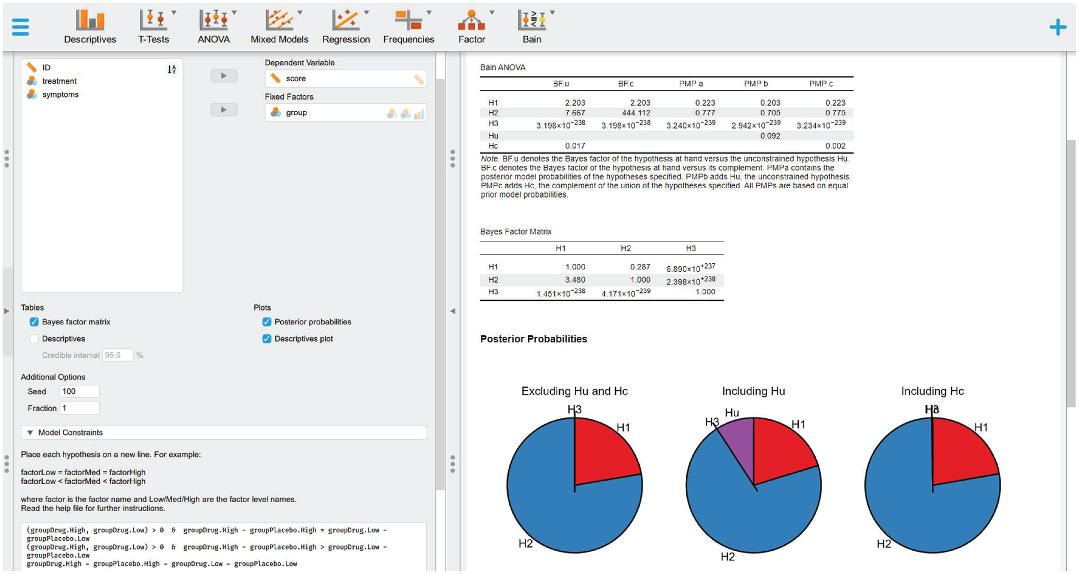
Selecting the variables, defining the informative hypothesis, and visualizing the results.

Then press Crtl+Enter (if you use a Windows PC) or Cmd+Return (if you use a Mac). JASP will start testing the informative hypothesis specified, and the results will be presented on the right panel, where a table called “Bain ANOVA” will appear (also reported in Table 1), containing all the information outlined in Box 3.

Table 1.

Bain Analysis of Variance

	BFu	BFc	PMPa	PMPb	PMPc
H1	2.21	2.21	0.221	0.201	0.221
H2	7.778	438.875	0.779	0.708	0.777
H3	3.20 × 10–238	3.20 × 10–238	3.20 × 10–239	2.91 × 10–239	3.20 × 10–239
Hu				0.091
Hc	0.018				0.002

Note: BFu = Bayes factor versus Hu; BFc = Bayes factor versus Hc; PMPa = posterior model probability excluding Hu and Hc; PMPb = posterior model probability including Hu; PMPc = posterior model probability including Hc. Because the values reported here are particularly high (e+) or particularly low (e–), scientific notation is used for convenience.

For more complete results, check the boxes on the left panel (Fig. 4) to display the “Bayes factor matrix” table (Table 2) and the “Posterior probabilities” plot (Fig. 5), which provide a pie chart of the proportion of the three PMPs reported in Table 1.

Fig. 5.

Posterior model probabilities (PMPs). Posterior model probabilities associated with the set of hypotheses tested (PMPa), also including Hu (PMPb) or Hc (PMPc).

Step 4a: interpret and report the results

In the following, we show how to interpret and report these results based on the indications outlined in Box 4.

All results obtained point in the same direction, indicating that H₂ is the hypothesis (or model) most supported by the data. H₂ is indeed associated with a largely higher relative PMP (Fig. 5) not only when considering the set of informative hypotheses tested (77.9%; Table 1: PMPa) but also when including Hc (77.7%; Table 1: PMPc). This last result, in particular, indicates that other models would not best represent the data (see Box 4, Question 1: Which of a set of hypotheses is the best?). In addition, H₂ resulted 438.857 times more likely than Hc (Table 1: BFc), thus showing strong support for this hypothesis compared with other possible models (see Box 4, Question 2: How much more likely a given hypothesis is relative to other possible explanations?). Finally, H₂ resulted 3.519 times more likely than H₁ (Table 2: BF₂₁) and 2.432 × 10⁺²³⁸ times more likely than H₃ (Table 2: BF₂₃), thus showing stronger support for H₂ relative to the other hypotheses tested (see Box 4, Question 3: How much more likely a given hypothesis is relative to another specific hypothesis?). Overall, these results indicate strong support for a higher treatment efficacy in the group presenting high levels of symptoms compared with the one presenting low levels of symptoms.

Table 2.

Bayes Factor Matrix

	H1	H2	H3
H1	1	0.284	6.91 × 10–237
H2	3.519	1	2.43 × 10–238
H3	1.45 × 10–238	4.11 × 10–239	1

Note: Because the values reported here are particularly high (e+) or particularly low (e–), scientific notation is used for convenience.

Step 5a: visual exploration of the data

Visually informative plots, such as estimation plots (Ho et al., 2019), raincloud plots (Allen et al., 2021), or plots representing model-estimated marginal means with confidence intervals (Garofalo et al., 2022), offer an immediate representation of the results based on a measurement scale that makes sense for the research question (Cumming, 2007, 2009; Cumming & Finch, 2005; Degni et al., 2022; Garofalo et al., 2022; Loftus & Masson, 1994; Masson, 2007). Thus, they can support data interpretation and possibly suggest new insights if our hypotheses result in a poor explanation of the data (see Box 4). Based on the software adopted, there are different options available to the user. In JASP, by clicking on the relative boxes available on the left panel, it is possible to obtain a “Descriptives” table and a “Descriptive plots,” respectively, containing descriptive statistics in text or visual format.

The results thus generated (Fig. 6) confirm that although the strongest difference is predictably between the two drugs and the two placebo groups, there is a higher difference between the drug and placebo treatments in the high-symptoms group compared with the low-symptoms group.

Fig. 6.

Visual exploration of the data in JASP.

Step-by-step tutorial in R

There are two ways to proceed with this example: (a) Open a new R script and use the following lines of code to play along with the tutorial or (b) open and use the file “BaIn_ANOVAinR.R” available on the OSF page (https://osf.io/dez9b/), which contains all the steps and code reported below.

Preliminary steps

Clear workspace

Before starting any new analysis, it is generally considered good practice to clear all the variables, data sets, functions, and so on possibly loaded in the R environment. To do that, you can use the rm() function as follows:

Install and/or load the necessary packages

Once R is installed, it comes with several built-in functions, such as sum(), which returns the sum of the values inserted between the brackets, or sqrt(), which returns the square root of all the values present in its arguments. To know what a function is used for, you can type “?” before the function name (i.e., ?sum) in the R console to open the help. Sets of functions that work together are usually grouped and contained in so-called packages (or libraries). For instance, sum() and sqrt() are part of the base package, which is automatically loaded when you use R. Packages for more specific analysis or plots have to be directly installed and loaded. For this tutorial, you need to install and load the bain package (Hoijtink, Mulder, et al., 2019), which contains all the functions needed to run Bayesian informative-hypotheses analyses. To do so, you can use the install.packages() function by running in R or RStudio the following line:

This line of code is needed only if you have not already installed this package. Once a package is installed on your computer, you can use the library() function to load it and access its functions. This loading needs to be done every time you start a new R session.

These two steps are required each time you need to use functions that are not part of base R but need to be loaded from an external package. In this tutorial, a few more packages will be used to generate plots or manipulate the data. These packages are not strictly required to run Bayesian informative hypotheses but can be very useful for several purposes. Each time, we suggest one of these packages, we explain their purpose and how to use them. However, the same results could be obtained with different packages.

Step 1a: load the data set

There are several options to load the file containing your data. The easiest one is to use the RStudio graphical user interface by clicking on “File → Import dataset” and choosing your file type (e.g., text, excel, SPSS; see Fig. 7). For this example, the data set is saved in a .txt file named “dataset_anova.txt.” To open it, go to “File → Import dataset → From Text (base)” and browse to the folder on your computer that contains the “dataset_anova.txt” file (downloaded from OSF page https://osf.io/dez9b/) and then click on “Import” to load the file. If you accept the default values, your data set will now appear in the R Environment with the same name as the original file name.

Fig. 7.

Loading the data set from the graphical user interface of RStudio.

If you prefer to use R code for loading a file, there are dedicated packages containing functions that can be used based on the file extension (e.g., a .txt file can be loaded with the read.table() function). An overview of such functions would go beyond the scope of this tutorial, but in the R script available online, you will find a few commented lines that can be used for this purpose.

Once the file has been loaded, an object named “dataset_anova” should appear in your R environment. By clicking on this object, the entire data set will appear (Fig. 8) containing the variables described above in the ANOVA Data Set section. The str() function can be used to familiarize with your data set. This function shows the structure of your data set and has the additional benefit of showing the data type for each variable:

Fig. 8.

Data set loaded in RStudio.

Step 2a: fit the model

The following code can be used to fit a linear model, with the function lm(), which returns estimated means for each level contained in the column “group.” The outcome of the fitted model will be stored in an object called “fit.” Note that the –1 is used to estimate the means for each level of the variables. The subsequent line uses the coef() function to store the means estimated by the model for each group and session in an object called “estimated”:

Step 3a: define and test informative hypotheses with bain

We can now set the hypotheses defined above and compare them. Before doing that, you can use the coef() function to take a look at the estimated means and their names because these are the variable names to use to define the informative hypotheses:

It is also important to know that many analyses require generating a series of random numbers for computational purposes. The bain package, in particular, uses sampling to compute BFs and PMPs. To get reproducible results, it is possible to use the set.seed() function, which sets a specific seed number from which the series of pseudorandom numbers is generated. Knowing the seed and the generator makes it always possible to reproduce the same output. It can be set to any number you like. A good practice to ensure the stability of your results is to repeat the analysis with different seeds and check whether the results are coherent. For this reason, we may use different seeds in the JASP and R examples and ensure that although slightly different, the same trend should emerge from both analyses. The following code can be used to set the seed to 123:

The following code can be used to test the informative hypotheses described above. The output is stored in an object called “results”:

In this code, the first argument “x” is a vector containing the estimated means for each group and condition, and the second argument “hypothesis” contains the hypotheses.

There are a few options available to display the results. The function print() returns in the console the main results or bain ANOVA table (Table 3):

Table 3.

Bain Analysis of Variance

	Fit	Com	BFu	BFc	PMPa	PMPb	PMPc
H1	0.097	0.044	2.212	2.212	0.225	0.204	0.224
H2	0.986	0.129	7.637	472.992	0.775	0.704	0.774
H3	0.000	0.012	0.000	0.000	0.000	0.000	0.000
Hu						0.092
Hc	0.014	0.871	0.016				0.002

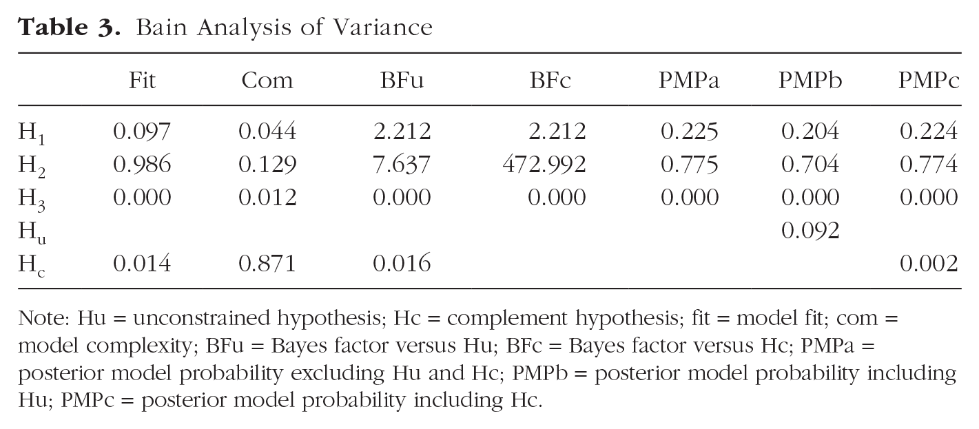
Note: Hu = unconstrained hypothesis; Hc = complement hypothesis; fit = model fit; com = model complexity; BFu = Bayes factor versus Hu; BFc = Bayes factor versus Hc; PMPa = posterior model probability excluding Hu and Hc; PMPb = posterior model probability including Hu; PMPc = posterior model probability including Hc.

This table is identical to Table 1 reported above in Step 4a except for the presence of fit (Fit) and complexity (Com) scores. For more information and definitions, see Box 3.

A pie chart displaying the three PMPs reported in Table 1 can be created using the pie() function or similar ones (Fig. 9). A detailed explanation of how to generate plots in R falls beyond the scope of the present article; however, the code used to generate Figure 9 is available on the R script associated with this example.

Fig. 9.

Posterior model probabilities (PMPs). PMPs associated with the set of hypotheses tested (PMPa), also including Hu (PMPb) or Hc (PMPc). The code used to generate this figure is available on the R script associated with this example.

To further support model selection, PMPs can also be compared via a BF matrix (Box 3) in which all hypotheses are compared with each other (Table 4). The following code can be used to extract this information from the “results” object created in the previous steps:

Table 4.

Bayes Factor Matrix

	H1	H2	H3
H1	1	0.275	6.87E+237
H2	3.639	1	2.50E+238
H3	0.000	0.000	1

Note: Because the values reported here are particularly high (e+) or particularly low (e–), scientific notation is used for convenience.

Step 4a: interpret and report the results

Please refer to Step 4a of the JASP example above for a complete guide on how to interpret and report these results.

Step 5a: visual exploration of the data

Please refer to Step 4a of the JASP example reported above for more on the importance of visual exploration of the data and how to interpret the results obtained.

In R/RStudio, in particular, several packages can be used for this purpose. Figure 10 shows a raincloud plot generated with the ggplot() and geom_rain() functions from the ggplot2 and ggrain packages (Allen et al., 2021). A detailed explanation of how to generate plots in R falls beyond the scope of the present article; however, the code used to generate Figure 10 is available on the R script associated with this example.

Fig. 10.

Visualizing the data. Raincloud plots of the data set representing the groups divided based on treatment (drug/placebo) and symptoms (high/low). The code used to generate this figure is available on the R script associated with this example.

The following line of code can be used to print a table with descriptive statistics:

Example B: Multiple Linear Regression

Let us assume we have already established that the previously tested anxiety treatment works (drug > placebo) and now wish to investigate if factors other than symptom severity can affect its effectiveness. To this aim, we want to evaluate on a continuous scale the impact of symptom severity along with drug dosage and age (independent variables). To this aim, we recruit 100 volunteers currently undergoing such anxiety treatment and obtain the same treatment-efficacy index used before (dependent variable). Because all our variables are continuous, multiple linear regression is a viable approach to test the influence that each independent variable and their combination can exert on the dependent variable.

The regression data set

The data set is composed of five columns: “ID” (containing participants’ identification number), “treatment.effect” (containing the treatment-efficacy score), “age” (containing participants’ age), “dosage” (containing participants’ drug dosage), and “symptoms” (containing participants’ symptoms). All variables are on a continuous scale.

The data were simulated by sampling 100 cases from a normal distribution using different means and standard deviations (M ± SD) for each variable: 0 ± 10 for the treatment effect, 40 ± 15 for age, 10 ± 5 for dosage, and 50 ± 5 for symptoms. All variables were subsequently standardized as z scores. This data set can be reproduced using the “creating the datasets.R” file available on the OSF page (https://osf.io/dez9b/).

The hypotheses

The first hypothesis poses that dosage has a higher impact than symptoms on treatment effect, which has a higher impact than age on treatment effect:

$${\mathrm{H}}_1:\mathrm{dosage}>\mathrm{symptoms}>\mathrm{age}.$$

The second hypothesis poses that symptoms have a higher impact than dosage on treatment effect, which has a higher impact than age on treatment effect:

$${\mathrm{H}}_2:\mathrm{symptoms}>\mathrm{dosage}>\mathrm{age}.$$

The third hypothesis poses that dosage and symptoms have a comparably higher impact than age on treatment effect:

$${\mathrm{H}}_3:\left(\mathrm{dosage},\mathrm{symptoms}\right)>\mathrm{age}.$$

For more on how to define informative hypotheses, see the Characteristics of the Informative Hypotheses section.

Step-by-step tutorial in JASP

The analysis presented in this section is performed using the bain module on JASP (JASP Team, 2021). The file “bain_REGRESSIONinJASP.jasps” available on the OSF page (https://osf.io/dez9b/) contains all the steps reported below and can be directly opened in JASP.

Preliminary steps

Follow the Preliminary Steps section of the JASP tutorial for Example A.

Step 1b: load the data set

Follow Step 1a of the JASP tutorial to load the file “dataset_regression.txt.” You will now visualize a spreadsheet containing the entire data set (Fig. 11) described above in The Regression Data Set section.

Fig. 11.

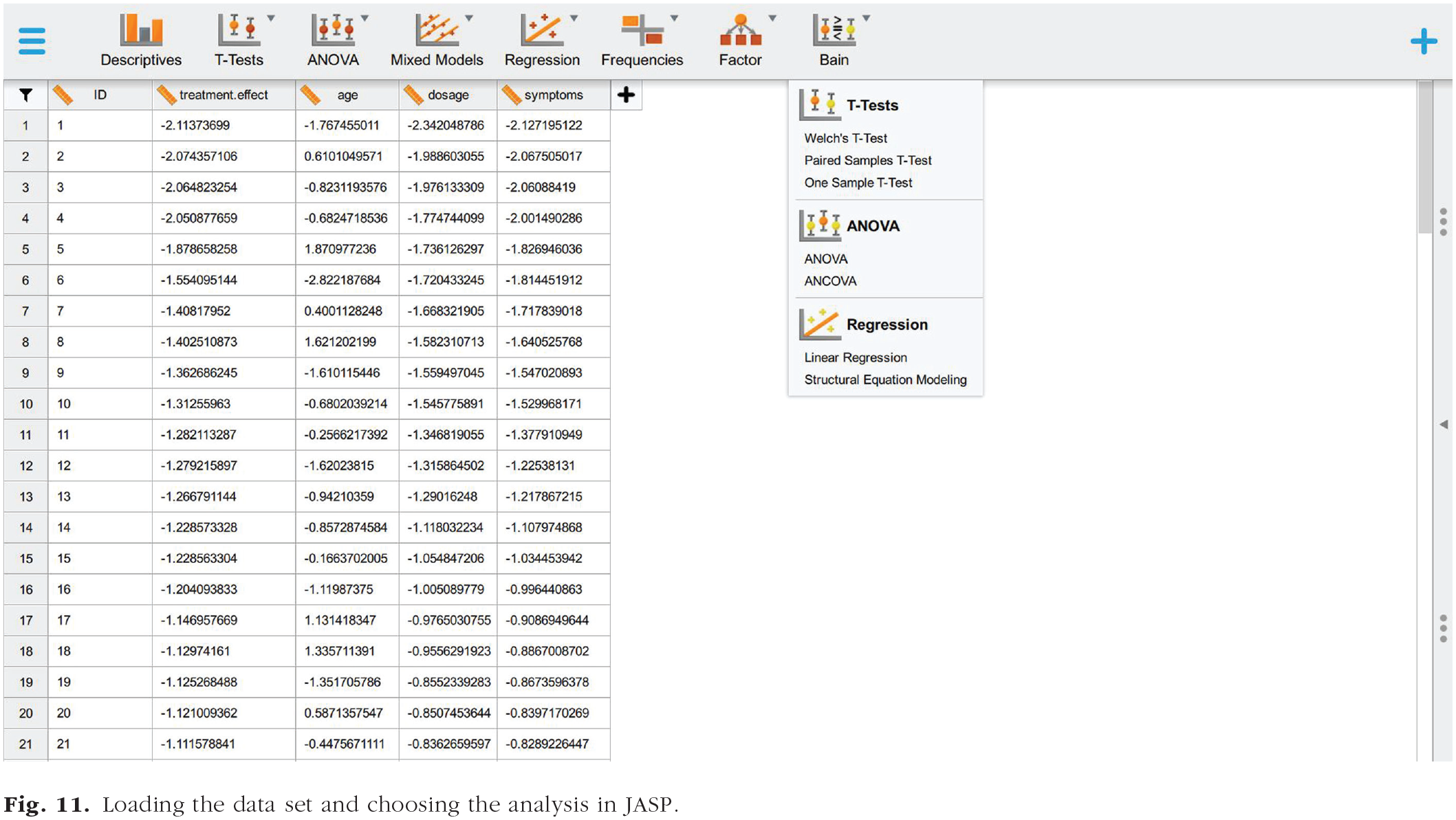
Loading the data set and choosing the analysis in JASP.

Step 2b: fit the model

By selecting “Linear Regression” in the bain menu (Fig. 11), you will be presented with a new graphical user interface that can be used to select the variables of interest (Fig. 12). Set the variable “treatment.effect” as the dependent variable and the variables “age,” “dosage,” and “symptoms” as covariates.

Fig. 12.

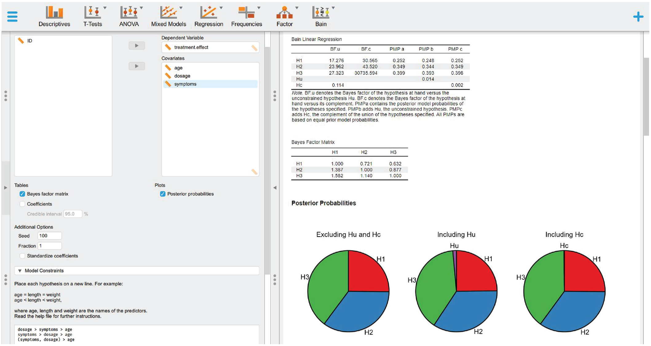
Definition of informative hypothesis and results.

Step 3b: define and test informative hypotheses with bain

Follow Step 3a of the JASP tutorial to set the hypotheses reported below, visualize the bain linear regression results (Table 5), display the BF matrix (Table 6), and plot the PMPs (Fig. 13):

Table 5.

Bain Linear Regression

	BFu	BFc	PMPa	PMPb	PMPc
H1	17.276	30.565	0.252	0.248	0.252
H2	23.962	43.52	0.349	0.344	0.349
H3	27.323	30,735.594	0.399	0.393	0.398
Hu				0.014
Hc	0.114				0.002

Note: BFu = Bayes factor versus Hu; BFc = Bayes factor versus Hc; PMPa = posterior model probability excluding Hu and Hc; PMPb = posterior model probability including Hu; PMPc = posterior model probability including Hc.

Table 6.

Bayes Factor Matrix

	H1	H2	H3
H1	1	0.721	0.632
H2	1.387	1	0.877
H3	1.582	1.14	1

Fig. 13.

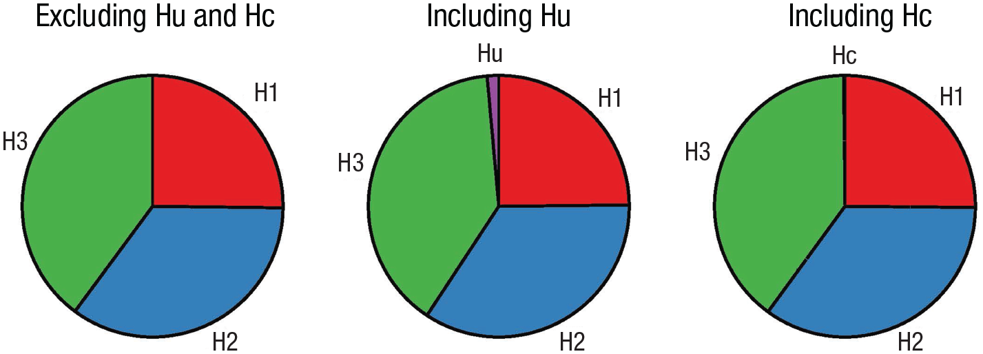
Posterior model probabilities (PMPs). PMPs associated with the set of hypotheses tested (PMPa), also including Hu (PMPb) or Hc (PMPc).

Step 4b: interpret and report the results

In the following, we show how to interpret and report these results based on the indications outlined in Box 4.

Although all results obtained point in the same direction, indicating that H₃ is the hypothesis most supported by the data, the strength of the evidence is not clear-cut in this case, thus suggesting careful consideration. H₃ is indeed associated with the highest relative PMP (Fig. 13) both when considering only the set of informative hypotheses tested (39.9%; Table 5: PMPa) and when including Hc (39.8%; Table 5: PMPc); however, such proportion is not strikingly different from that associated with H₂ (34.9%). Despite this, the three hypotheses do seem to be good models for the data (Hc = 0.02%; see Box 4, Question 1: Which of a set of hypotheses is the best?). In addition, although all hypotheses resulted to be more likely than the complement hypothesis (Table 5: BFc), H₃ reported a much stronger support in this regard, being 30,735.594 times more likely than Hc (see Box 4, Question 2: How much more likely a given hypothesis is relative to other possible explanations?). Finally, H₃ proved to be 1.582 times more likely than H₁ (Table 6: BF₃₁) and 1.14 times more likely than H₂ (Table 6: BF₃₂), thus showing weak but still present support in its favor (see Box 4, Question 3: How much more likely a given hypothesis is relative to another specific hypothesis?). Overall, these results indicate that although both symptoms and dosage undoubtedly appear to have a stronger impact on treatment efficacy than age, whether the two have a significantly different impact is yet to be clarified.

Step 5b: visual exploration of the data

Unfortunately, at the moment of writing, the bain module does not allow generating a plot of the model data directly. As an alternative, the standard module for running linear regression can be used for this aim. To do that, select the “Regression” module and then “Linear Regression” (Fig. 14). You will be now presented with a new graphical user interface that can be used to select the variables of interest (Fig. 14). Set the variable “treatment.effect” as the dependent variable and the variables “age,” “dosage,” and “symptoms” as covariates. Then, go to the “Plots” section on the bottom left panel and check the “Partial plots” box.

Fig. 14.

Using the “Regression” module to obtain partial regression plots.

Partial regression plots can be used to display the relationship between the dependent variable and one independent variable at a time while controlling for the presence of other independent variables in the model (Fox & Weisberg, 2019). By visual inspection only (Fig. 14), it is possible to appreciate a few crucial things: (a) A linear estimation of the relationship between the variables appears appropriate; (b) dosage and symptoms appear to have the strongest relationship with the treatment effect, whereas no relationship with age emerges; and (c) there is an outlier score that needs to be taken into account for a correct interpretation of the results (Altman & Krzywinski, 2016; Greco et al., 2019).

Step-by-step tutorial in R

There are two ways to proceed with this example: (a) Open a new R script and use the following lines of code to play along with the tutorial or (b) open and use the file “BaIn_REGRESSIONinR.R” available on the OSF page (https://osf.io/dez9b/), which contains all the steps and code reported below.

Preliminary steps

Follow the Preliminary Steps section of the R tutorial for Example A.

Step 1b: load the data set

Follow Step 1a of the R tutorial to load the file “dataset_regression.txt” and visualize the data set described above in The Regression Data Set section.

Step 2b: fit the model

The following code can be used to fit a linear model with the function lm(), which returns estimated coefficients for each independent variable:

Step 3b: define and test informative hypotheses with bain

Follow Step 3a of the R tutorial to test the hypotheses reported below, print the main results of the bain linear regression (Table 7), display the BF matrix (Table 8), and plot the PMPs (Fig. 15):

Table 7.

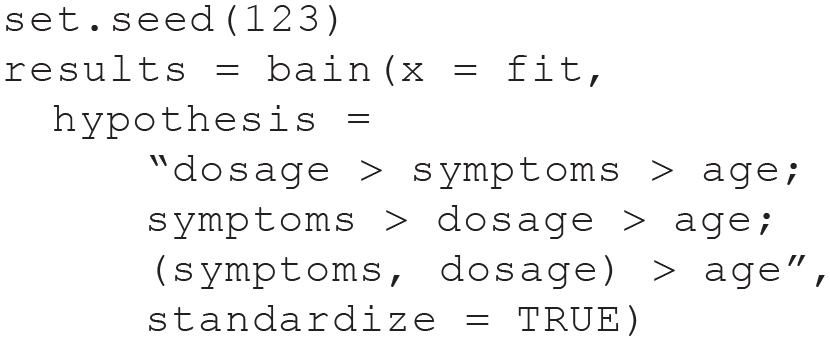
Bain Regression

	Fit	Com	BFu	BFc	PMPa	PMPb	PMPc
H1	0.418	0.013	31.418	53.267	0.364	0.36	0.364
H2	0.452	0.019	24.113	43.194	0.28	0.276	0.279
H3	1	0.033	30.684	1.18e+09	0.356	0.352	0.355
Hu						0.011
Hc	0.173	0.965	0.179				0.002

Note: Hu = unconstrained hypothesis; Hc = complement hypothesis; fit = model fit; com = model complexity; BFu = Bayes factor versus Hu; BFc = Bayes factor versus Hc. PMPa = posterior model probability excluding Hu and Hc; PMPb = posterior model probability including Hu; PMPc = posterior model probability including Hc. Because the values reported here are particularly high (e+) or particularly low (e–), scientific notation is used for convenience.

Table 8.

Bayes Factor Matrix

	H1	H2	H3
H1	1	1.303	1.024
H2	0.767	1	0.786
H3	0.977	1.272	1

Fig. 15.

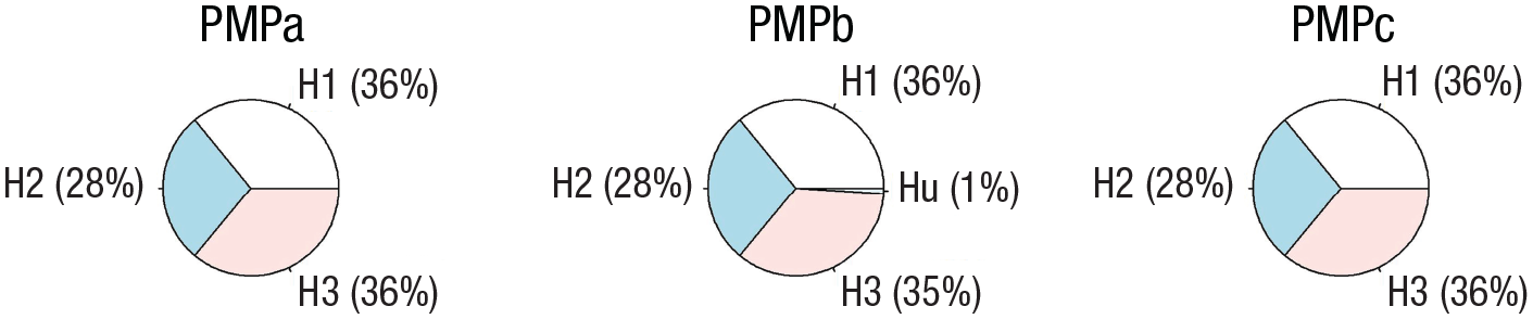
Posterior model probabilities (PMPs). PMPs associated with the three hypotheses (PMPa), also including Hu (PMPb) or Hc (PMPc). The code used to generate this figure with the pie() function is available on the R script associated with this example.

Step 4b: interpret and report the results

Please refer to Step 4b of the JASP example for a complete guide on how to interpret and report these results.

Step 5b: visual exploration of the data

Please refer to Step 4b of the JASP example reported above for more on the importance of visual exploration of the data and how to interpret the results obtained. In R/RStudio, in particular, the function avPlots() from the package car can be used to generate partial regression plots (Fig. 16). A detailed explanation of how to generate plots in R falls beyond the scope of the present article; however, the code used to generate Figure 16 is available on the R script associated with this example.

Fig. 16.

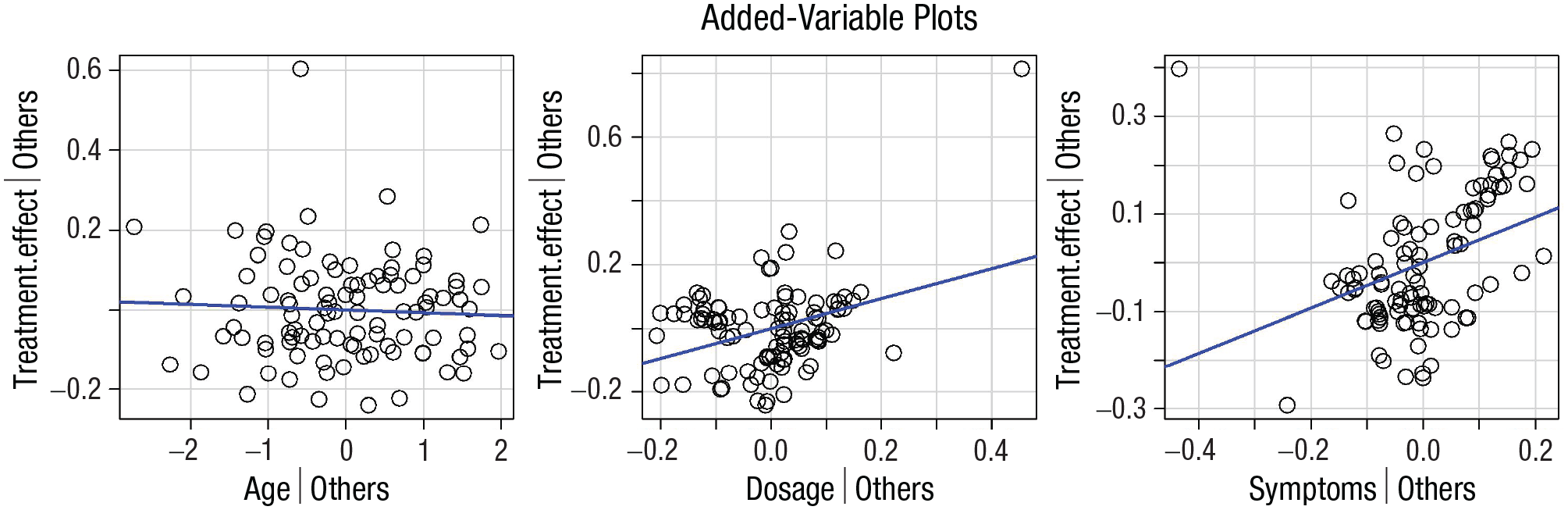
Visualizing the data. Added-variable plots of the linear regression model. Each panel represents the dependent variable (treatment effect) on the y-axis and one of three independent variables (age, dosage, and symptoms, respectively) on the x-axis. The regression line in blue shows the association between the two variables displayed net of all other independent variables in the model.

Conclusion

Especially in—but not limited to—psychological and cognitive sciences, experimental hypotheses do not fit the conventional definitions of null (A = B) and alternative hypotheses (A ≠ B). Most times, actual research expectations involve very specific predictions that could be defined in terms of equality (=) and inequality (> or <) constraints among the parameters. In other words, these are informative hypotheses that could be better tested via a model-comparison approach than via classical hypothesis testing (Gu et al., 2018; Hoijtink, 2012; Hoijtink, Mulder, et al., 2019; Kerr, 1998). Bayesian informative-hypothesis testing offers a powerful and easy way to directly compare predefined hypotheses through a Bayesian model-selection procedure in which each hypothesis represents a potential explanation or expectation for a phenomenon. Following the five steps outlined in the present tutorial, this can be easily achieved using two of the most commonly adopted software for statical analysis: JASP and R/RStudio. In the present tutorial article, we encourage the adoption of such an inferential approach whenever specific research hypotheses are present (Garofalo et al., 2022) to overcome old—and not necessarily more accurate—standards in statistical practice and embrace a richer and more meaningful interpretation of research results (Calin-Jageman & Cumming, 2019; Garofalo et al., 2022; Hoijtink et al., 2016).