How Do I Know What My Theory Predicts?

Abstract

To get evidence for or against a theory relative to the null hypothesis, one needs to know what the theory predicts. The amount of evidence can then be quantified by a Bayes factor. Specifying the sizes of the effect one’s theory predicts may not come naturally, but I show some ways of thinking about the problem, some simple heuristics that are often useful when one has little relevant prior information. These heuristics include the room-to-move heuristic (for comparing mean differences), the ratio-of-scales heuristic (for regression slopes), the ratio-of-means heuristic (for regression slopes), the basic-effect heuristic (for analysis of variance effects), and the total-effect heuristic (for mediation analysis).

Researchers are often interested in the existential question of whether something exists: Should an effect be in a model? Is there an interaction? Are there side effects of the drug? One has to assume something exists in order to estimate it (and in not estimating other things, one presumes that they do not exist). So it would be nice to have a measure of evidence for something existing versus not existing. Significance testing is a tool that is commonly used for this purpose; however, nonsignificance is not itself evidence that something does not exist. On the other hand, a Bayes factor can provide a measure of evidence for a model of something existing versus a model of it not existing (Etz & Vandekerckhove, 2018; Morey, Romeijn, & Rouder, 2016). Thus, evidence for existence versus nonexistence is put on a symmetric footing. This article gives practical guidance on using Bayes factors (readers who have no background in their use might find it helpful to first read Dienes, 2014, or Dienes & McLatchie, 2018, for an introduction congruent with the approach taken here). After introducing the problem of using Bayes factors when there is limited relevant prior information to inform a model of the target effect, I provide a number of heuristics for this situation.

A model, as the term is used here, is a representation of the predictions of a theory. The model indicates the plausibility of different population values of the parameter postulated to exist; that is, the model of H ₁ is a probability distribution of these parameter values. The contrast model can simply state that the parameter does not exist; this is the model of H ₀ . These two models can then be used to calculate a Bayes factor, and hence the evidence for one model versus the other, which in this case is the evidence that something exists versus does not. The effect sizes that the theory predicts must be specified in order to construct a model of H₁. This is what many researchers might find difficult. There can be evidence that something does not exist only given a claim of how big it could be, if it did exist. But how does one know what effect size one’s theory predicts?

Data collected to test a theory give information about the size of an effect, should it exist. Thus, one might be tempted to use the data that are used for testing the theory to also specify the effect size predicted. But this is double counting, and forbidden by the mathematical derivation of a Bayes factor (comment by D. V. Lindley in “Discussion of the Paper by Aitkin,” 1991, pp. 130–131). To put this another way, in order for theory and data to be able to clash, the model of H₁ should not be constructed from the same information that it is tested against. If the same data are used to generate the predictions of a theory and to test them, the theory cannot be severely tested (cf. Popper, 1963). How, then, can one determine the range of effect sizes consistent with a theory? The bulk of this article describes several heuristics that can be used to constrain predicted effect sizes even in the absence of relevant past studies. First, though, to provide some background, I give an example in which a predicted range of effect sizes is based on relevant past research, describe the types of models I used for calculating Bayes factors in the examples presented, and illustrate the general approach using a case in which there is no relevant past research.

Example of Relevant Past Research Helping to Define the Effect Expected

Cavanagh et al. (2013) found that a 2-week mindfulness-of-breathing intervention increased mindfulness by 0.2 Likert rating points on the Five Facet Mindfulness Questionnaire. Suppose that a researcher decides that it would be useful to try as a conceptual replication a 2-week mindfulness-of-walking intervention, given the theory that mindfulness of breathing and of walking engage the same process, namely, mindfulness. In her sample, she finds that the walking intervention is associated with a mean difference (from the control group) of 0.1 Likert units on the mindfulness questionnaire. If she uses this mean difference obtained from the sample as the basis for constructing her model of H₁, she has double-counted it: first for forming the model’s predictions and then again for testing them. Choosing the predicted mean effect in the model of H₁ to be the same as the data’s mean results in a pseudo-Bayes factor and puts the theory at least risk of being shown to be wrong.

Instead, the researcher could use the theory that mindfulness interventions focusing on breathing and focusing on walking promote mindfulness in the same way (they are both examples of mindfulness training). She could then use the past study on mindfulness of breathing to predict the effect size for the mindfulness-of-walking study. Note that the theory that two things belong to the same class does the work in making that prediction. Hence, the theory can take credit (or blame) in light of the evidence for this H₁ versus H₀; in other words, the theory can be tested. In general, an important question is when a theory can take credit for the results of a test of a particular model of H₁. A common case is precisely the one illustrated here: A theory can take credit (or blame) when the theory claims that two things belong to the same class, and that claim is used to construct H₁. But often one does not know what prior studies are relevant, or thinks none are. How does one construct a model of H₁ then? This is the problem I address in this article. Before presenting several heuristics for dealing with this problem, I first describe the sort of models of H₁ I use in discussing those heuristics and then consider an example of the approach.

Models

To simplify discussion, I primarily use a model of H₁ that is very commonly used for constructing Bayes factors. This model consists of a distribution centered on zero, and the problem is to determine the approximate size of effect predicted, that is, the distribution’s scale factor; half of the distribution (below 0) may be removed to represent a theory making a directional prediction (given that the predicted direction has been defined as positive). The mode of the distribution is set at zero in order to represent in a simple way that smaller effect sizes are more probable than larger ones; this approach can be useful given a literature that habitually overestimates effect sizes.

In this article, I use mostly a half-normal distribution, and the problem is to determine its standard deviation (see, e.g., Dickey, 1973; Dienes & McLatchie, 2018). The standard deviation is set to the rough scale of the effect expected. Thus, the problem of specifying the model of H₁ reduces to specifying the effect size expected. I notate a Bayes factor based on a half-normal distribution with a mode of 0 and a standard deviation of r as BF_HN(0,r). I have made available online a calculator (Dienes, 2008, 2018) that can be used with this model of H₁; to obtain the Bayes factor, one needs only to add the observed effect size and its standard error. Another commonly used distribution is the Cauchy (or half-Cauchy) distribution (used in JASP: Rouder, Speckman, Sun, Morey, & Iverson, 2009; van Doorn et al., 2019); again, to obtain a Bayes factor given this distribution, one needs to set its scale factor, that is, to determine the rough scale of the effect expected. I notate a Bayes factor based on a Cauchy distribution with a mode of 0 and a scale factor of d as BF_C(0,d). For convenience, I use the term scale factor to refer to both the scale factor of a Cauchy distribution and the standard deviation of a normal distribution._. For the same scale factor, the normal and the Cauchy distributions give very similar Bayes factors, though the Cauchy slightly favors H₀ more than the normal distribution does (Dienes, 2017a; see Box 1 for further discussion on using the Cauchy vs. the normal distribution). None of these models may be appropriate in any given case (e.g., see Dienes, 2014; Gronau, Ly, & Wagenmakers, 2019); however, they are good enough approximations sufficiently often that they serve as good vehicles for discussing the heuristics this article focuses on (see Dienes & McLatchie, 2018, and Rouder et al., 2009, for justifications of these models).

Box 1.

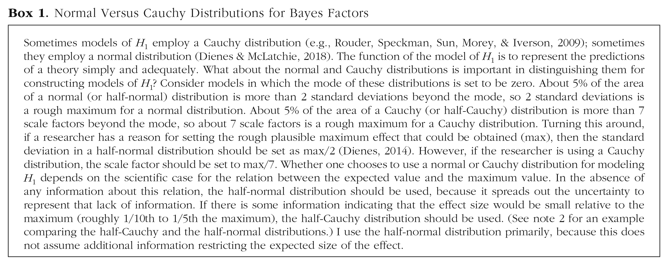
Normal Versus Cauchy Distributions for Bayes Factors

Sometimes models of H1 employ a Cauchy distribution (e.g., Rouder, Speckman, Sun, Morey, & Iverson, 2009); sometimes they employ a normal distribution (Dienes & McLatchie, 2018). The function of the model of H1 is to represent the predictions of a theory simply and adequately. What about the normal and Cauchy distributions is important in distinguishing them for constructing models of H1? Consider models in which the mode of these distributions is set to be zero. About 5% of the area of a normal (or half-normal) distribution is more than 2 standard deviations beyond the mode, so 2 standard deviations is a rough maximum for a normal distribution. About 5% of the area of a Cauchy (or half-Cauchy) distribution is more than 7 scale factors beyond the mode, so about 7 scale factors is a rough maximum for a Cauchy distribution. Turning this around, if a researcher has a reason for setting the rough plausible maximum effect that could be obtained (max), then the standard deviation in a half-normal distribution should be set as max/2 (Dienes, 2014). However, if the researcher is using a Cauchy distribution, the scale factor should be set to max/7. Whether one chooses to use a normal or Cauchy distribution for modeling H1 depends on the scientific case for the relation between the expected value and the maximum value. In the absence of any information about this relation, the half-normal distribution should be used, because it spreads out the uncertainty to represent that lack of information. If there is some information indicating that the effect size would be small relative to the maximum (roughly 1/10th to 1/5th the maximum), the half-Cauchy distribution should be used. (See note 2 for an example comparing the half-Cauchy and the half-normal distributions.) I use the half-normal distribution primarily, because this does not assume additional information restricting the expected size of the effect.

For the sake of discussion, in this article I treat a Bayes factor greater than 3 as good enough evidence for H₁ over H₀, a Bayes factor less than 1/3 as good enough evidence for H₀ over H₁, and a Bayes factor between those values as being nonevidential (cf. Jeffreys, 1939). However, there are no real cutoffs; these are just rough guidelines adopted because in practice decisions often have to be made. Further, we as a community may (and I think should) decide that cutoffs of 3 and 1/3 are not good enough for many scientific problems: Schönbrodt, Wagenmakers, Zehetleitner, and Perugini (2017) recommended a cutoff of at least 5 (or 1/5); the cutoff for Cortex’s (2019) Registered Reports is 6 (or 1/6); and Benjamin et al. (2018) recommended 20 (or 1/20) for one-off studies. The results of the Bayesian approach and significance testing can be aligned as best as possible (even though there is no monotonic transformation between Bayes factors and p values) by using a cutoff of 3 for Bayes factors if .05 is the cutoff for significance, by using a cutoff of 6 for Bayes factors if .02 is the cutoff for significance, and by using a cutoff of 20 for Bayes factors if .005 is the cutoff for significance.

Example of Defining the Predicted Effect When There Is No Relevant Past Research

Now consider an example in which there is no relevant past research on which to base the model of H₁. Theory A claims that autistic subjects will perform worse on a novel task than control subjects will. Theory B claims that the two groups will perform the same. Chance performance on the task (i.e., baseline) is 0%, and the maximum score is 50%. The autistic group (n = 30) scores 8% above baseline (SE = 6%), and the control group (n = 30) scores 10% above baseline (SE = 5%). The difference between the groups (2%) is nonsignificant, t(58) = 0.25, p = .80, Cohen’s d = 0.05. One reaction to this result might be that the nonsignificance means Theory B is supported. But a nonsignificant result does not distinguish between evidence for H₀ over H₁ and the lack of much evidence either way. To know if there is evidence for H₀ over H₁, we need to know the size of the effect we could be trying to pick up. In other words, how should we model H₁?

One temptation might be to use a default model of H₁, for example, the model JASP gives by default for a t test (i.e., a Cauchy distribution with a scale factor of 0.7 Cohen’s d units). The resultant JZS Bayes factor, BF_{C(0,0.7 Cohen’s d units)}, is 0.27. On the face of it, we have evidence for Theory B, because the Bayes factor is less than 1/3. But there is no such thing as a default theory, so there cannot be a default model of H₁ (Etz, Haaf, Rouder, & Vandekerckhove, 2018; Lee & Vanpaemel, 2018; Rouder, Morey, Verhagen, Province, & Wagenmakers, 2016; see Box 2 for further discussion in the broader context of using raw vs. standardized effect sizes). In fact, the data themselves indicate that it is too rash to conclude that there is good evidence for Theory B over Theory A. The control group scored 10%, so given Theory A, which says the autistic group will perform somewhere between the control group’s level and 0, the difference between the autistic and the control groups cannot be more than about 10%. Modeling H₁ as a half-normal distribution with a standard deviation of 5% (i.e., maximum/2) results in BF_HN(0,5%) = 0.94: Thus, there is no evidence one way or the other. This is clearly a reasonable conclusion because the standard error of the difference between the groups is 7.8%, about as big as the maximum possible difference. There cannot be evidence for or against a difference in the population if the standard error of the sample difference is as large as the maximum plausible difference. One can think of this as a floor effect on the difference score: If the maximum plausible difference indicates that the sample difference cannot be greater than the standard error of the sample difference, there is a floor effect.

Box 2.

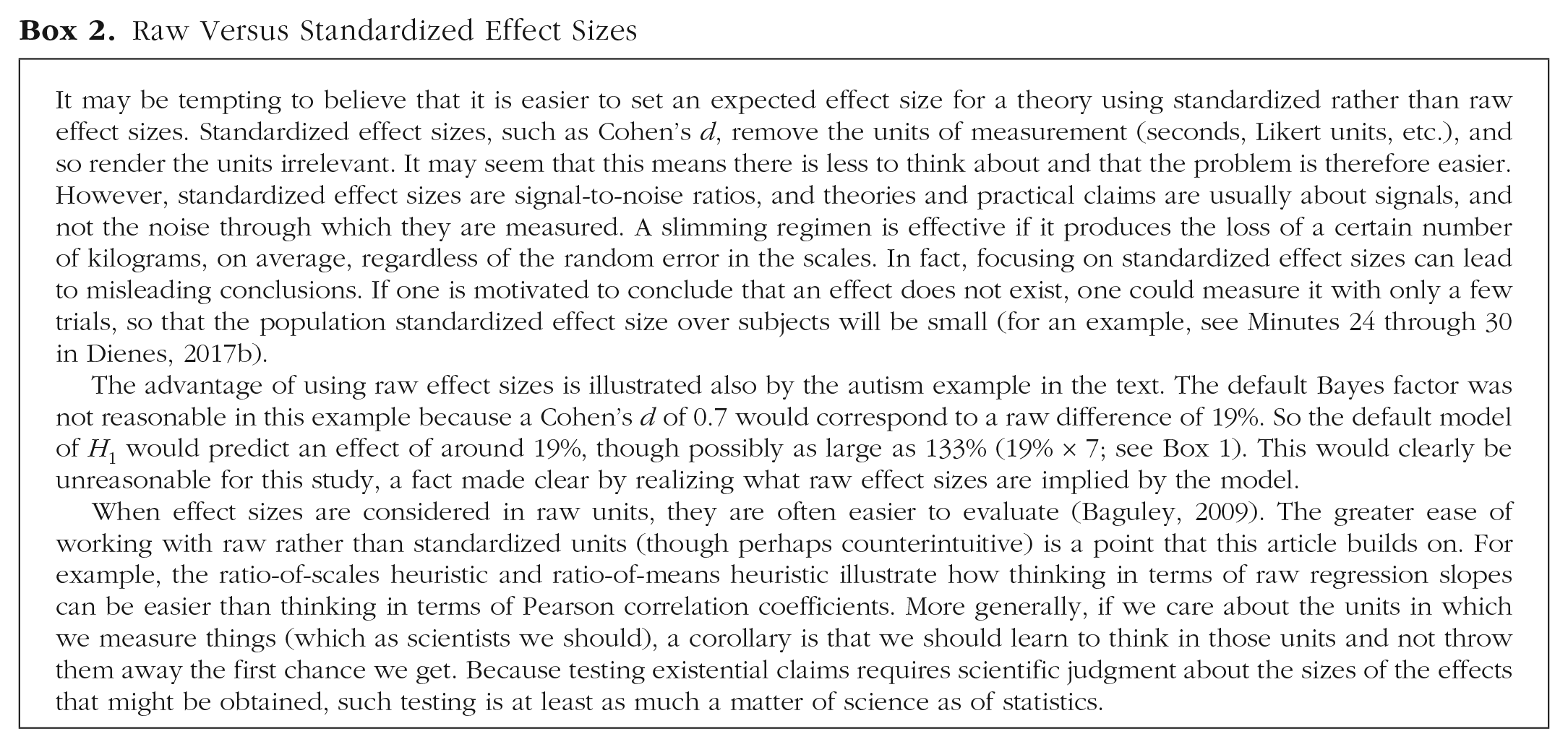
Raw Versus Standardized Effect Sizes

It may be tempting to believe that it is easier to set an expected effect size for a theory using standardized rather than raw effect sizes. Standardized effect sizes, such as Cohen’s d, remove the units of measurement (seconds, Likert units, etc.), and so render the units irrelevant. It may seem that this means there is less to think about and that the problem is therefore easier. However, standardized effect sizes are signal-to-noise ratios, and theories and practical claims are usually about signals, and not the noise through which they are measured. A slimming regimen is effective if it produces the loss of a certain number of kilograms, on average, regardless of the random error in the scales. In fact, focusing on standardized effect sizes can lead to misleading conclusions. If one is motivated to conclude that an effect does not exist, one could measure it with only a few trials, so that the population standardized effect size over subjects will be small (for an example, see Minutes 24 through 30 in Dienes, 2017b). The advantage of using raw effect sizes is illustrated also by the autism example in the text. The default Bayes factor was not reasonable in this example because a Cohen’s d of 0.7 would correspond to a raw difference of 19%. So the default model of H1 would predict an effect of around 19%, though possibly as large as 133% (19% × 7; see Box 1). This would clearly be unreasonable for this study, a fact made clear by realizing what raw effect sizes are implied by the model. When effect sizes are considered in raw units, they are often easier to evaluate (Baguley, 2009). The greater ease of working with raw rather than standardized units (though perhaps counterintuitive) is a point that this article builds on. For example, the ratio-of-scales heuristic and ratio-of-means heuristic illustrate how thinking in terms of raw regression slopes can be easier than thinking in terms of Pearson correlation coefficients. More generally, if we care about the units in which we measure things (which as scientists we should), a corollary is that we should learn to think in those units and not throw them away the first chance we get. Because testing existential claims requires scientific judgment about the sizes of the effects that might be obtained, such testing is at least as much a matter of science as of statistics.

Notice that the control group’s mean was used to inform the maximum plausible difference between the autistic and control groups. How does this relate to the principle, stated earlier, that the mean difference in the data cannot be used to predict the same mean difference? In this case, the information used to determine the maximum plausible difference was not exactly the information that was tested (though they were correlated). The information used constrained inference in a plausible way: A floor effect appropriately rendered the data nonevidential (see Fig. 1a). Further, if there had been no floor effect, using the control group to define a maximum difference would have given full scope for either theory to clash with the data (i.e., to be shown to be wrong): If the standard error of the difference between the groups had been small, similar performance of the autistic and control groups would have been evidence refuting Theory A (see Fig. 1b), and near-chance performance of the autistic group would have been evidence refuting Theory B (see Fig. 1c). Thus, we have cheated information out of the data in a useful way that does not impair theory testing. That is, this procedure can provide what Popper (1963) called a severe test of relevant theories. A severe test is one in which a theory is made to “stick its neck out”; if the theory is wrong, it can easily be found to be wrong.

Fig. 1.

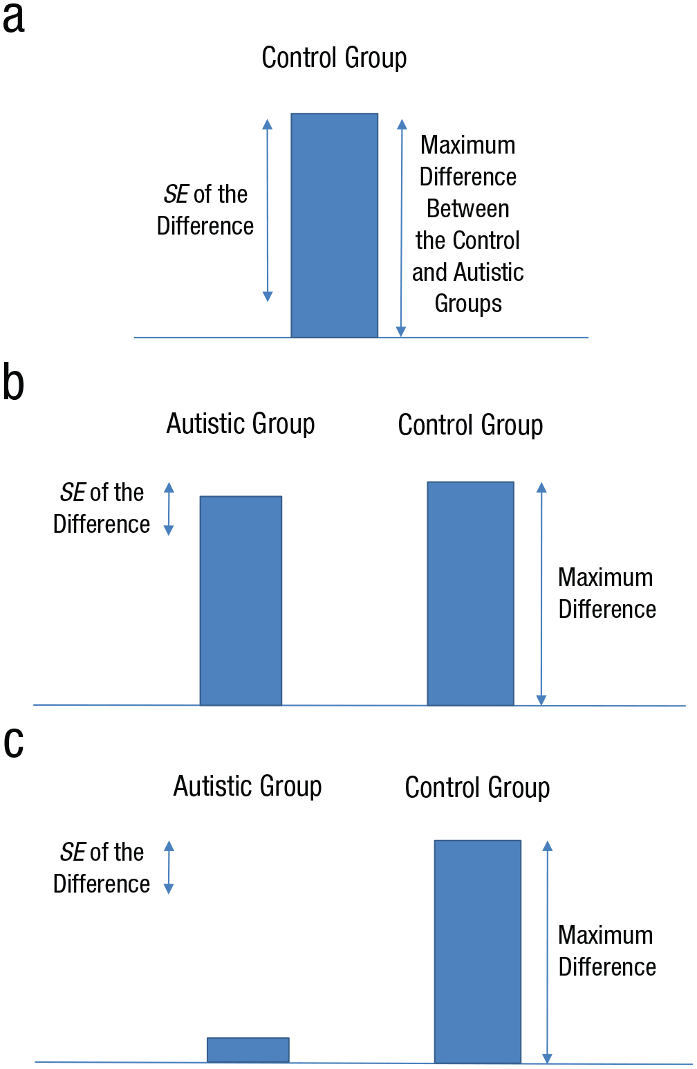
Using the control group’s mean to define the maximum plausible difference between the autistic group and control group. If this procedure shows that there is an effective floor effect (a), in the sense that the observed standard error of the difference between the groups is as large as any difference that could be expected, the results are nonevidential, as no sample difference can be far enough away from the floor defined by the standard error of the difference. However, if the standard error of the difference is small enough, the actual difference between groups can strongly count against either a theory that predicted a difference (b) or a theory that predicted no difference (c): Theory can still clash with the data.

The Heuristics

In the following sections, I generalize these considerations and present a set of heuristics for obtaining a ballpark estimate for a reasonable predicted effect size. For each Bayes factor, I present a robustness region, notated as “RR [min, max],” where min is the minimum scale factor that leads to the same qualitative conclusion (i.e., good evidence for H₁ over H₀ if BF > 3; good evidence for H₀ over H₁ if BF < 1/3; and not much evidence at all otherwise), and max is the maximum scale factor that leads to the same conclusion ¹ (see Box 3). (If the conclusion is that there is not much evidence at all, min will always be 0, and if the conclusion is that there is good evidence for H₀ over H₁, max will always be infinity. If a scale has a maximum, the maximum difference possible for the study is the scale’s maximum; if, for example, the scale is from 0 to 7 and the maximum for a Bayes factor to be consistent with a given evidential standard exceeds 7, one could notate the maximum difference in the robustness region as “> 7.”) None of the heuristics are guaranteed to produce sensible answers in context; scientific judgment is always needed for all aspects of model building. Nonetheless, a heuristic can do its job merely if it puts one in the right ballpark; if the robustness region is about the width of the ballpark (in particular, if the range of scientifically plausible scale factors is contained within the robustness region), then the conclusion is safe. A heuristic will often also help a researcher see what range of scale factors is scientifically plausible, as I show later. In the current example, the robustness region for a half-normal distribution model of H₁ is RR_1/3<BF<3 [0, 28%]. That spans the whole ballpark (a standard deviation of 28% corresponds to a plausible maximum difference of 56%), so the conclusion that there is no evidence one way or the other is safe. Recall that the scale factor is the key aspect of the model, indicating roughly how big the population difference between autistic and nonautistic individuals is; a given scale factor indicates that a plausible population difference lies between 0 and about twice that scale factor (for a normal or half-normal distribution).

Box 3.

Robustness Checking

For all statistical analyses, including those using Bayes factors, it is worth considering how robust conclusions are to reasonable changes in assumptions. When Bayes factors are used to test a theory, the model of H1 represents the predictions of the theory. But there could be several equally good ways of modeling H1 to represent the same theory. Thus, a conclusion would be robust only if most of the models would lead to the same qualitative conclusion. In previous work (Dienes, 2015, Appendix 12.1), I used different distributions (uniform vs. normal vs. half-normal) to show that the precise shape of the distribution can make little difference to conclusions in individual cases when the distributions represent roughly the same scientific assumptions. Given just one form of distribution, such as a half-normal, the conclusion is robust if the range of scale factors (standard deviations) leading to the same qualitative conclusion roughly spans or contains the range of scientifically plausible values. JASP produces a graph showing the Bayes factor for different scale factors. In interpreting this graph, the issue is not whether all the Bayes factors agree in the conclusion implied, but rather whether the range of scientifically plausible scale factors is roughly contained in a range of scale factors that lead to the same conclusion. This notion is formalized in the robustness region, which is a type of minimultiverse (Steegen, Tuerlinckx, Gelman, & Vanpaemel, 2016). There are no precise rules yet to say how robust is robust enough, and probably there should not be. But if the robustness region is always provided, readers can determine if it contains their preferred rough scale factor. If a conclusion is not robust enough, in principle more data can be collected until it is more robust. With Bayes factors, it is fine to continue collecting data until the evidence is good enough (Rouder, 2014, 2019). The robustness regions in this article were calculated by iteratively entering different scale factors in my Bayes factor calculator (Dienes, 2008, 2018) until the limits of good-enough evidence were reached (cf. McLatchie, 2018). One way to ensure some robustness is to use a stopping rule for achieving a degree of evidence that clearly exceeds what is taken to be good enough. For example, one may run subjects until the Bayes factor is greater than 10 or less than 1/10, and then report the robustness region with respect to cutoffs of 5 and 1/5.

Now I discuss each of the heuristics in turn: the room-to-move heuristic, the ratio-of-scales heuristic, the ratio-of-means heuristic, the basic-effect heuristic, and finally, the total-effect heuristic for mediation.

The room-to-move heuristic

The hypothetical example of autistic and control groups’ performance on a novel task illustrates the heuristic of using one condition to define the rough maximum difference that could be obtained between conditions: The one condition shows how much room there is for the other condition to move in order to satisfy the constraints of the theory. For a real example, consider the theory that people pursue relationships to obtain a mix of eroticism and nurturance. In a polyamorous relationship, one can have different partners for different needs; thus, the partners in a polyamorous relationship might satisfy the particular needs they are assigned to better than would the partner in a monogamous relationship, in which one partner has to satisfy all needs. Balzarini, Dharma, Muise, and Kohut (2019) investigated the relative quality of polyamorous and monogamous relationships. On a scale from 1 to 7, people in monogamous relationships rated their partner’s nurturance as 5.85. In the subset of polyamorous people who were without a self-defined primary partner, when relationship length was controlled for, the mean nurturance rating for the partner they mainly lived with was 5.80. The standard error of the difference between the two groups was 0.11, and the difference between the groups was not significant according to a t test, t(≈2500) = 0.42 (see Table 5 of Balzarini et al.).

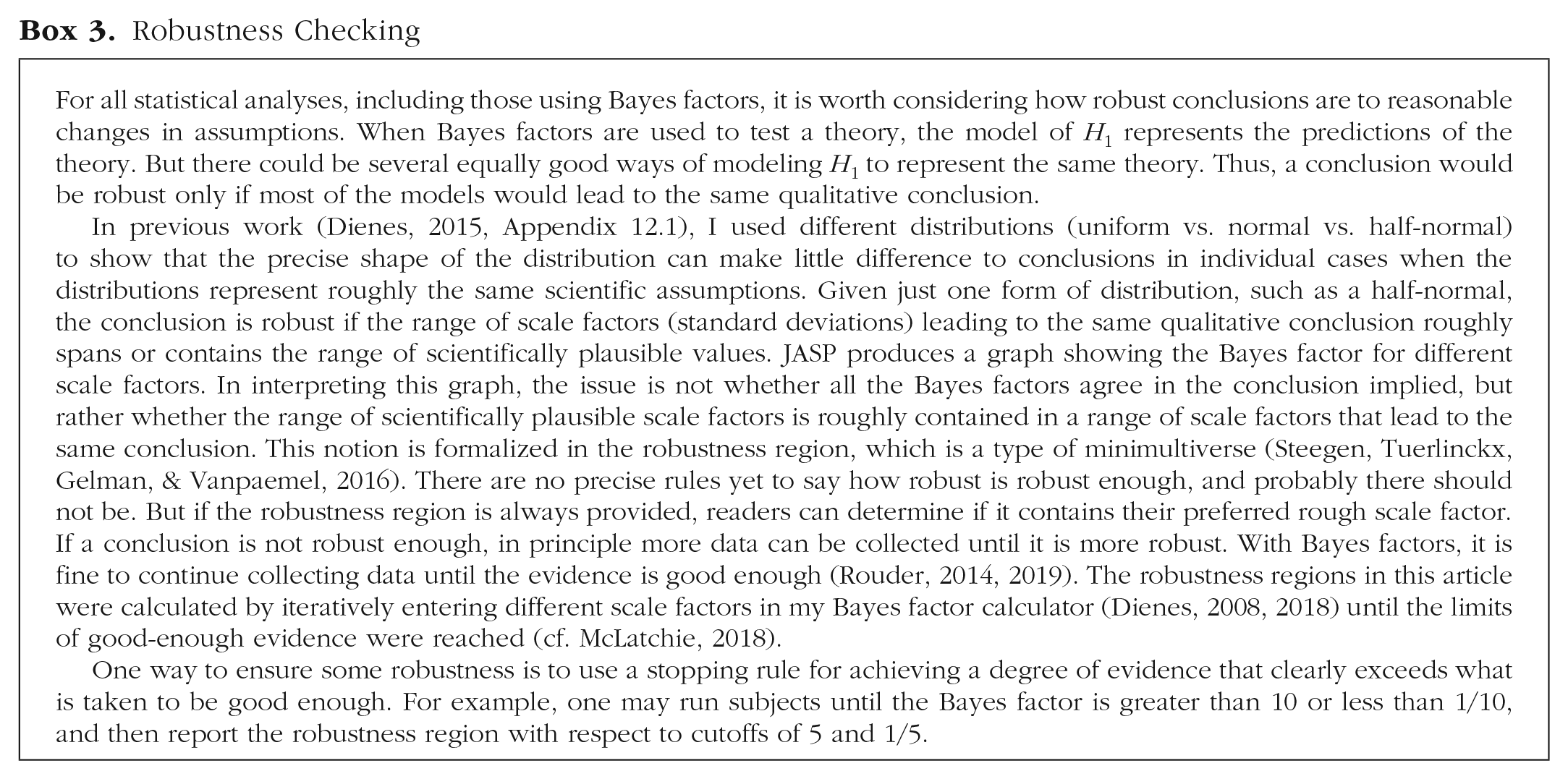
But, again, nonsignificance does not mean there is evidence for no difference. To define the evidence, the scale of the effect predicted by H₁ needs to be determined. How should H₁ be modeled? Given the monogamous group’s ratings, how different could the polyamorous group’s ratings be? The monogamous group rated their partner’s nurturance as 5.85, on average, and the top of the scale was 7, so the maximum possible positive difference was about 1.15 units (see Fig. 2); in other words, 1.15 units was the room to move for the polyamorous group. So, to model H₁ using the room-to-move heuristic, we can use a half-normal distribution with a standard deviation of 0.58 rating units (i.e., maximum/2). The resulting Bayes factor indicates that the data provide evidence for H₀ over H₁, BF_HN(0,0.58) = 0.13, RR_BF<1/3 [0.22, > 6].

Fig. 2.

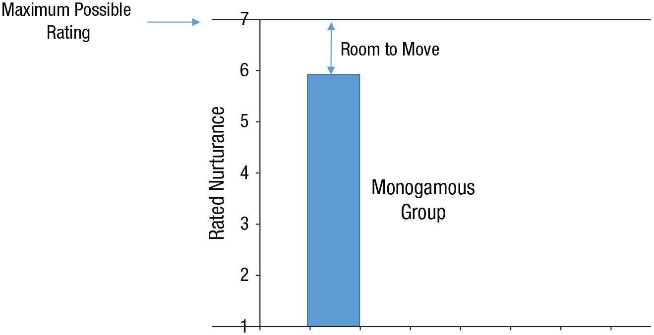
Calculating the room to move. In the study by Balzarini, Dharma, Muise, and Kohut (2019), the monogamous group rated their partner’s nurturance as 5.85, on average, and 7 was the top of the scale. Therefore, when polyamorous people without a self-defined primary partner rated a partner’s nurturance, their ratings could not be more than 1.15 units higher than those of the monogamous group; in other words, the polyamorous group had 1.15 units of room to move. Thus, the data from one group can provide constraints on the difference between groups. This is the concept underlying the room-to-move heuristic.

We can assess the robustness of this conclusion by taking into account information from the other polyamorous couples in the study, that is, those with defined primary and secondary partners. These polyamorous couples’ ratings of the nurturance of the partner they mostly lived with were 0.57 units higher, on average (SE = 0.10), than the monogamous couples’ ratings of their partners. Thus, 0.57 is a more informed estimate of the sort of difference that could be expected. This value is very similar to the value derived by applying the room-to-move heuristic to the ratings of the monogamous couples (a similarity that cannot in general be guaranteed) and is well within the robustness region.

Why not take the polyamorous group’s mean as given and see how much room there was for the monogamous group’s ratings to be lower than that? In that case, the room to move would have been about 4.85 (from 5.85 to the bottom of the scale, 1), and that could in principle have made a difference in the conclusion drawn (though, in fact, it did not in this case). It is best to choose the direction that gives the smallest room to move, because that will show up any floor or ceiling effects. So in this case, it was justified to use the monogamous group’s data to set the room to move.

The room-to-move heuristic is based on a point estimate from one group. For example, we have assumed that 5.85 is a reasonably precise estimate of the nurturance of the monogamous group’s partners. This approach has the advantage of simplicity, but it also disregards the uncertainty in the estimate. In this case, the standard error of the estimate is 0.03 nurturance units, so the estimate is precise enough. The function of the heuristic is to put us in the right ballpark; the question then is the width of the robustness region. The robustness region in this case includes all reasonable rooms to move.

In order to analyze interactions, Gallistel (2009) suggested taking a key simple effect as the maximum size the difference in simple effects could be, that is, as the maximum size of the interaction (see also Dienes, 2014). This idea constitutes applying the room-to-move heuristic to an interaction effect. For example, Raz, Shapiro, Fan, and Posner (2002) tested highly hypnotizable people on the Stroop task, either after giving them no suggestion or after giving them a suggestion that the words on the screen were written in a meaningless foreign script. The suggestion reduced the Stroop interference effect. As this was the first time the study was run, there was no prior information about how effective the suggestion should be. In the no-suggestion condition, Raz et al. found that response times for incongruent and neutral words were 860 ms and 748 ms, respectively. In the suggestion condition, the corresponding response times were 669 and 671 ms. In the no-suggestion condition, the interference effect was 112 ms (860 ms – 748 ms). That is the simple effect of word type for the no-suggestion condition. In the suggestion condition, the interference effect was –2 ms (669 – 671). That is the simple effect of word type for the suggestion condition.

Given that the interference effect was 112 ms in the no-suggestion condition, the most suggestion could plausibly have reduced interference was about 112 ms. That is the only room in which the effect could move. Therefore, we can model the H₁ for the interaction of word type and suggestion as a half-normal distribution (a directional distribution because suggestion should reduce, not increase, the interference effect) with a standard deviation of 56 ms (i.e., maximum/2 = 112/2). So we have predicted the size of the effect. In fact, the raw interaction effect was 114 ms (112 – –2 ms). Now we need to find the standard error of the effect: Raz et al.’s reported interaction test was F(1, 30) = 29.35, which corresponds to t(30) = √29.35 = 5.42. Therefore, the standard error for the interaction, calculated by dividing the raw effect size by the obtained t, was 21 ms (114 ms/5.42). The Bayes factor obtained with the Dienes (2008, 2018) calculator, BF_HN(0,56), is 2.86 × 10⁵, RR_BF>3 [4.3, 4 × 10⁴]. Thus, the data provide evidence that the suggestion reduced Stroop interference, as the robustness region contains all remotely plausible scale factors. (In fact, a meta-analysis by Parris, Dienes, & Hodgson, 2013, indicated that the suggestion roughly halves the interference effect, so the model of H₁ based on past data that my lab now preregisters is precisely also the model that would be given by the room-to-move heuristic—e.g., Palfi, Parris, McLatchie, Kekecs, & Dienes, 2018). Note here the advantage of using raw units, milliseconds. If fewer trials of the Stroop test were run, the expected standardized effect size would change, but the fact that the effect of suggestion is approximately to halve the raw interference effect would remain invariant.

The ratio-of-scales heuristic

The ratio-of-scales heuristic may be useful when correlating variables or regressing one variable on another. The task is to determine if a simple version of a theory can be tested by making a correspondence between two low points on the scales and two high points. Notice that the task is not to determine the spread of the data for each variable, but rather to determine what a simple theory would predict given the meaning of the scale points.

For an illustrative example, consider a study by Lush et al (2019), in which people estimated the time when a tone occurred. In fact, the tone sounded 250 ms after a button press. Application of Bayesian cue-combination theory to time estimation suggests that in this paradigm, the experienced time of the tone should be pulled toward that of the button press in proportion to the observer’s relative precision, which was measured on a scale from 0% to 100%. One way to test the theory would be to determine if the shift in the estimated time of the tone correlated with subjects’ relative precision: The theory predicts that the higher the precision, the greater the shift. What size correlation could we expect? .2? .6? .8? Who knows? If we think in terms of raw units, prediction becomes easier. The maximum possible shift in timing was all the way over to the button press, that is, a shift of 250 ms. In the simplest version of the theory, this is what would happen in the case of subjects with relative precision of 100%, and there would be no shift among subjects with relative precision of 0%. So the raw slope of shift against precision in this case is the length of the scale for shift (250 – 0 ms) divided by the length of the scale for precision (100% – 0%), that is, 2.5 ms per percent, the ratio of the scales (see Fig. 3). This is the maximum slope that would occur if the only mechanism was the one postulated and it operated with complete effectiveness. Thus, the ratio-of-scales heuristic gives the maximum slope that could be expected. Hence, we can model H₁ for the raw regression slope with a half-normal distribution with a standard deviation of 1.25 ms per percent (2.5/2). ² In fact, Lush et al. obtained a raw regression slope of 0.59 ms per percent (SE = 0.26), t(68) = 2.23, p = .029, BF_HN(0,1.25) = 4.74, RR_BF>3 [0.16, 2.1]. The robustness region ranges from very small to almost the maximum slope plausible, so the evidence for there being a slope is robust to the value of the scale factor in this case.

Fig. 3.

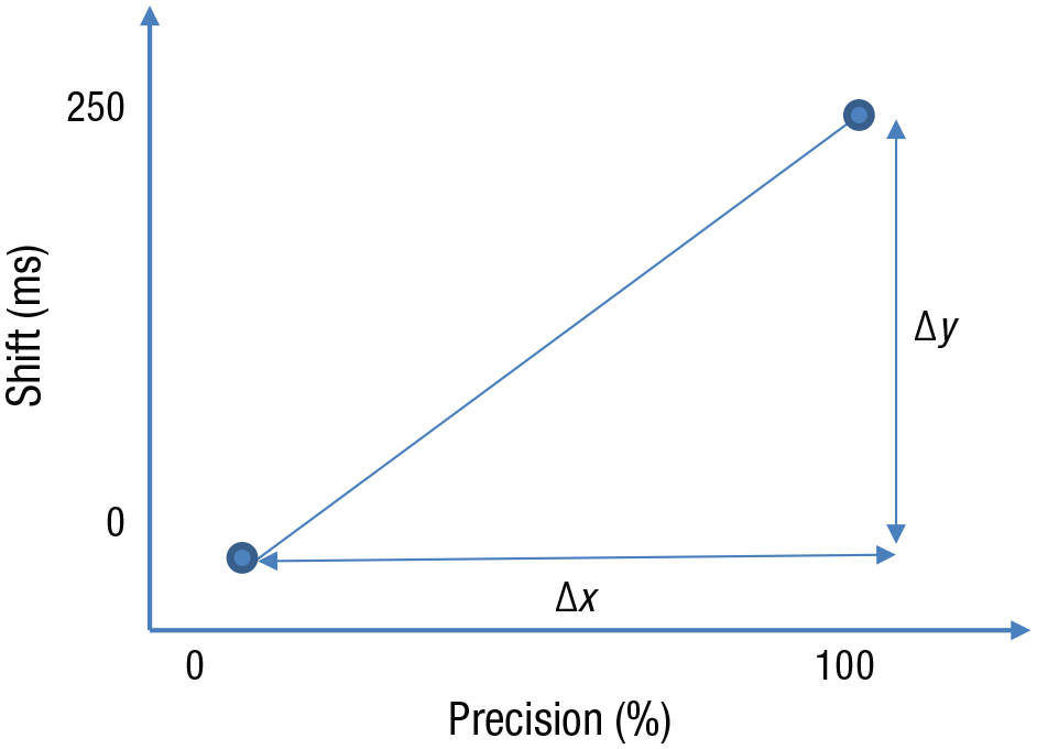
Illustration of the ratio-of-scales heuristic for regression (or correlation). The maximum slope predicted by the theory tested in Lush et al. (2019) is the ratio of the lengths of the two scales, that is, 250 ms divided by 100%, or 2.5 ms per percent.

On the basis of construal theory, Monin, Levy, and Kane (2017) predicted that women who were high in marital satisfaction—but not men and women low in marital satisfaction and men high in marital satisfaction—would experience more distress on days when they perceived their partner as experiencing more suffering. The dependent variable was how distressing it was to see the partner suffering, measured on a scale from 1 (not at all stressful) to 4 (very stressful). The independent variable was perceived physical suffering of the partner on a scale from 1 (did not suffer) to 10 (suffered terribly). If distress increased with perceived suffering in a simple way, and subjects used most of the scale points a fair amount of the time, they would report no suffering on days they reported no distress; that is, the line for the relationship between distress and suffering would start at (1,1). In addition, terrible suffering would go with the most distress, so the line would go through (10,4). A first approximation of the line’s slope would be calculated as (4 – 1)/(10 – 1), indicating an increase of 0.33 distress units per suffering unit. But any variable that affected distress independently of suffering would reduce the relationship.

Applying the ratio-of-scales heuristic, we can treat the ratio of the scales’ ranges as a rough maximum. That is, we can model the H₁ for the relation of distress to suffering as a half-normal distribution with a standard deviation of 0.17 (half the maximum). Monin et al. (2017) believed that the relationship between marital distress and partner suffering would hold well for partners with high marital satisfaction but not for those with low satisfaction. ³ The observed slope for high-satisfaction males was 0.03 distress units per suffering unit (estimated from the authors’ graph), SE = 0.02. The Bayes factor indicates that the data are nonevidential, BF_HN(0,0.17) = 0.66, RR_1/3<BF<3 [0, 0.35]. The maximum scale factor in the robustness region is high given that the plausible maximum is around 0.33, so the conclusion that the data are nonevidential is robust. Therefore, the authors’ conclusion that “men who were high in marital satisfaction experienced heightened daily distress irrespective of their perceptions of level of spousal suffering” (p. 383) is not supported if “irrespective” is read as meaning that in this group, daily distress had no relation to perceived suffering.

The ratio-of-means heuristic

Some scales, for example, reaction times or d′ (discrimination), have no obvious high point to relate to a high point of another variable. It may be difficult theoretically to fix an a priori plausible correspondence between two scales when one (or both) lacks such a high point. In these cases, the ratio-of-means heuristic can be helpful. For example, Salvador et al. (2018) regressed a measure of thought suppression (difference between conditions in percentage correct) against ability to discriminate whether a no-think cue was present (d′); the latter measure was taken to be a measure of conscious perception. The raw slope was –5.7% per d′ unit, ⁴ t(42) = 0.77, p = .45, “indicating that people’s ability to discriminate masked cues did not predict their [thought suppression]” (pp. 194–195), and that thought suppression was triggered unconsciously.

However, the nonsignificant result does not justify the conclusion of no relation between thought suppression and conscious perception. (There are arguments against first-order d′ being a valid measure of conscious perception—see Dienes & Seth, 2018; but the authors’ assumptions can be accepted for the sake of determining what tests would be relevant for those assumptions.) What strength of relation could be predicted if both measures depended on conscious perception of the cue? Given that d′ goes from 0 to infinity, what high level of d′ should correspond to a high degree of thought suppression? The ratio-of-scales heuristic is hard to apply in this case. But we may use a ratio-of-means heuristic, which is akin to applying the room-to-move heuristic to each variable. The theory that mean thought suppression and d′ both depend on a single knowledge base (e.g., conscious perception) predicts that they should go to zero together (see Fig. 4). Thus, the slope for their relation should be the ratio of their means, 6%/0.35, or 17% per d′ unit. This is a maximum because it assumes that all systematic variance is due to conscious knowledge. Thus, we can model H₁ as a half-normal distribution with a standard deviation of 8.5% per d′ unit (17%/2). With these assumptions, the Bayes factor, BF_HN(0,8.5), is 0.43, RR_1/3<BF<3 [0, 12], and the data are nonevidential. The robustness region reaches a moderately high value of the slope (given an estimated maximum of 17), so the conclusion that there is not enough evidence is somewhat robust to the scale factor. ⁵

Fig. 4.

Illustration of the ratio-of-means heuristic. For these imaginary data points, let the rectangle mark the mean level of thought suppression and mean level of d′. The theory that both variables depend on a single knowledge base predicts that they should go to zero together, so the expected slope is the ratio of the means. The y-axis variable is the difference in percentage correct between two conditions, so it has a true zero; d′ has a true zero when discrimination is at chance.

The basic-effect heuristic

One can often take the size of a basic effect as a rough scale for how much that effect could be manipulated. This approach can often by useful for analysis of variance. Martin and I (Martin & Dienes, 2019) used this principle to test whether different types of hypnotic induction were differentially effective in changing response to suggestion. If people were given 10 hypnotic suggestions, and coded as having passed or failed each suggestion (i.e., as having sufficiently experienced the suggested effect or not), would different inductions have different pass rates? The bigger the effect any induction has on response, the more inductions may differ among themselves in the magnitude of their effects, much as adult shoe sizes differ more among themselves than baby shoe sizes do. Therefore, the scale factor for the model of H₁ for the difference between different inductions was set as the difference between no induction and the standard induction. A standard hypnotic induction increases the pass rate by 1.46 suggestions out of 10, so that was set as the scale factor for the difference between different inductions. An indirect induction had been argued to be especially powerful, and we tested that claim. Past research showed a difference between standard and indirect inductions of 0.01 passes (SE = 0.25). The resultant Bayes factor, BF_HN(0,1.46), was 0.20, RR_BF<1/3 [0.9, > 10]. Thus, the data provide evidence that the effect of an indirect induction is not different from the effect of a standard induction, on average.

Ziori and I (Ziori & Dienes, 2015) investigated how gender and attractiveness of facial stimuli may affect implicit learning of sequences of those stimuli. The average level of implicit learning, that is, the average increase in accuracy above baseline after training (6%), was taken as a rough scale by which that effect could be modulated by the manipulations, and was used as the scaling factor for all effects in the three-way 2 × 2 × 2 analysis of variance (every effect with 1 degree of freedom, whether a main effect, interaction, or simple effect, can be expressed as a contrast in raw units). In another study (Caspar, Desantis, Dienes, Cleeremans, & Haggard, 2016), my colleagues and I used the height of an event-related potential component as the maximum that the component could be modulated (on the basis of past experience with how much such components are typically modulated).

One could broaden this heuristic further to a reference-effect heuristic, whereby the size of one effect (perhaps multiplied by a constant) is used as a basis for the expected size of another effect (cf. Palfi et al., 2018). For example, in a functional MRI study, one could use a standard contrast to define the effect expected for a contrast of interest. In a subliminal-perception experiment, one can test if the level of conscious perception is at chance only if one knows how much conscious perception would be expected. Thus, the level of conscious perception that leads to a given level of priming in a conscious condition could provide the expected level of conscious perception that would lead to the same level of priming when the stimuli are presented in a potentially subliminal manner (if priming were actually based on conscious perception; Dienes, 2015). If a previous experiment used response times and the current study is using d′, there may be a standard effect that could be used to convert response times to d′ (cf. Dienes, 2014, Supplementary Material, Appendix 1, Section 2).

The total-effect heuristic for mediation

In a mediation analysis, one might want to know whether the effect of X on Y is mediated completely, partially, or not at all by M (see Fig. 5). In frequentist methods, evidence for some mediation is provided if the first and second indirect effects are both significant (the method of joint significance; e.g., Woody, 2011). Recently, Yzerbyt, Muller, Batailler, and Judd (2018) argued that this method should be preferred to the currently more common use of a single index of the indirect effect. Whichever approach is used, the main problem for frequentist methods arises in trying to determine if there is evidence for full mediation or no mediation, because each of those claims depends on evidence for an H₀. This problem can be solved by rephrasing the method of joint significance in terms of Bayes factors (see Nuijten, Wetzels, Matzke, Dolan, & Wagenmakers, 2015, for a different approach). Conclusions regarding the indirect effect can be based on the Bayes factors for the individual (first and second) indirect effects: (a) If the Bayes factor for either individual indirect effect is less than 1/3, then there is evidence for no mediation; (b) if the Bayes factor for both individual indirect effects is greater than 3, then there is at least partial mediation; and (c) if one Bayes factor is insensitive and the other is greater than 1/3, then there is no evidence either way. Because these indirect effects are tested using regressions, the ratio-of-scales or ratio-of-means heuristic may provide a model of H₁.

Fig. 5.

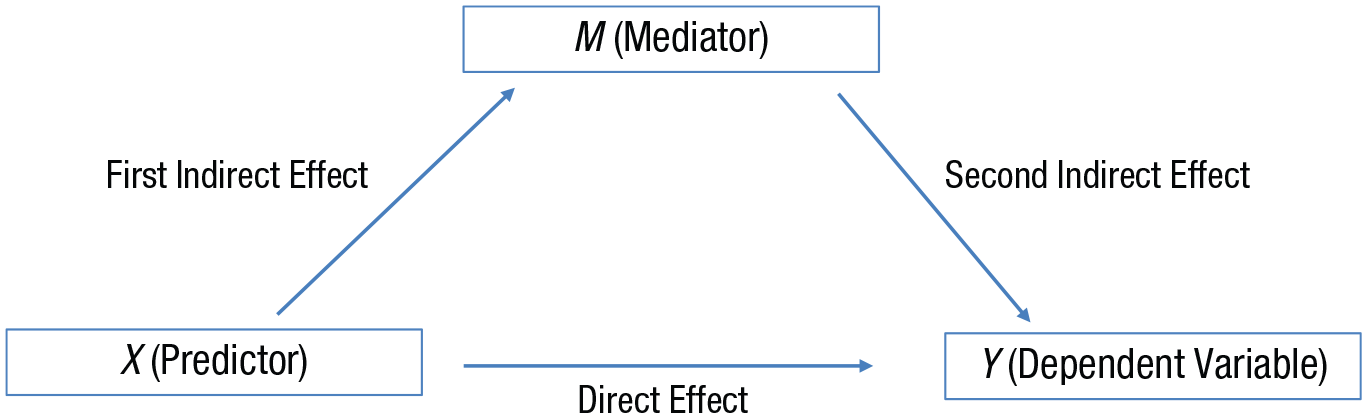
A model of the effect of X on Y, potentially through a mediator, M. The equations defining the three variables are as follows: M = a₁ + b₁ × X; Y = a₂ + b₂ × X + b₃ × M; and Y = a₃ + b₄ × X. The a_i terms indicate that the regression slopes are in raw units. Given these equations, b₁ = first indirect effect, b₃ = second indirect effect, b₁ × b₃ = indirect effect; b₄ = total effect, and b₂ = direct effect.

Now take the case of testing for full mediation. Assume that there is evidence for an indirect effect. Full mediation can then be tested using the Bayes factor for the direct effect: (a) If the Bayes factor is greater than 3, then there is not full mediation; (b) if it is less than 1/3, then there is full mediation; and (c) if it is between 1/3 and 3, then there is no evidence either way about full mediation. To test the evidence for a direct effect, there is a simple heuristic that can be used. Mathematically, the total effect is the sum of the direct effect and the indirect effect. Thus, one possible theory is that the total effect is the maximum that could be expected for the direct effect. ⁶ To test this theory, we can model H₁ for the direct effect using the uniform distribution [0, total effect]. This is the total-effect heuristic. (We use a uniform distribution in this case because there is typically no reason to expect that the direct effect will be closer to 0 than to the total effect or vice versa.)

Consider a study in which openness to experience (X) is used to predict relationship satisfaction (Y), with richness of fantasies as a mediator (M); all three variables are rated on Likert scales. The total effect is 0.10 Likert unit of Y per Likert unit of X (SE = 0.02), t(450) = 5.00, p < .001 (i.e., X predicts Y), and the direct effect (i.e., with M partialed out) is 0.04 (SE = 0.03), t(450) = 1.33, p = .18. A typical but incorrect temptation is to conclude that the significant total effect and nonsignificant direct effect mean there is complete mediation: Openness to experience increases relationship satisfaction only via increasing the richness of fantasies. Indeed, not only is the direct effect nonsignificant, but also the JZS default Bayes factor for the direct effect, BF_C(0,.35) = 0.11, indicates there is evidence for H₀ and seems to confirm the claim of complete mediation. But the default scale factor, r = .35, is arbitrary. The maximum that the direct effect could be (given the theory that openness increases fantasy richness, which in turn increases relationship satisfaction) is the total effect, that is, 0.10 Likert unit per Likert unit. If we use the total-effect heuristic, the Bayes factor for the direct effect, BF_U[0,.10], is 1.62, RR_1/3<BF<3 [0, 0.5]. ⁷ Thus, the data are nonevidential, and robustly so over any plausible upper limit for the uniform distribution.

Discussion

A scientist tries to explain the world. The explanations can be tested via their predictions. For such a test, we need a model of the predictions—minimally, the sort of effect size, ideally in raw units, that is expected. Even when there is no prior work in the field, there are heuristics that enable setting minimal constraints on what can be expected. As long as these constraints put one in the right ballpark, and help define what the ballpark is, evidential conclusions follow if they are robust to the range of plausible values (i.e., about the width of a ballpark). Notice that the Bayes factors I have used in this article do not involve H₁s with point predictions; they respect the vagueness of real psychological theory in representing a range of possible effect sizes. Considering robustness means making sure that conclusions are similar throughout the plausible range of the width of that plausible range.

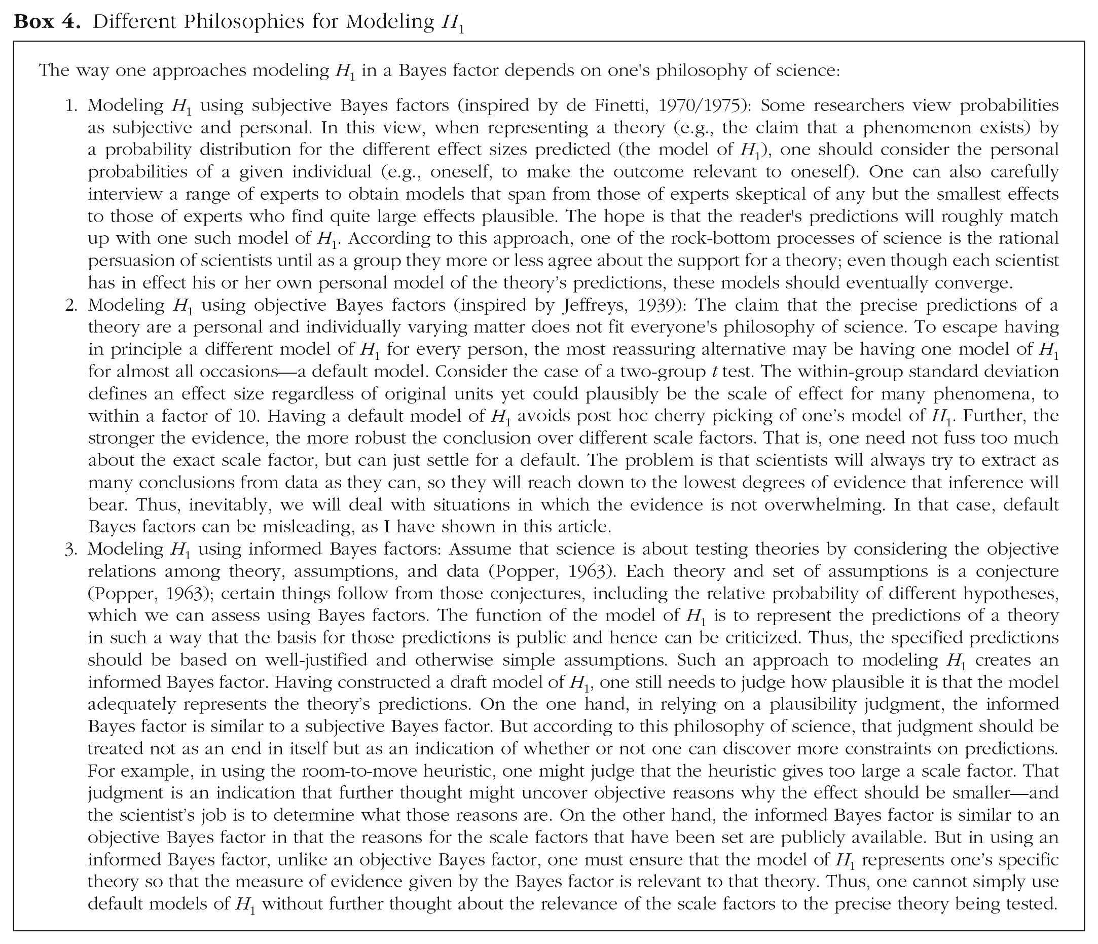
There are no strict default effect sizes in theory testing, and hence no objective or default Bayes factors (see Box 4 for the range of philosophies concerning Bayes factors, not just the one argued for in this article). A proposed default Bayes factor is not an invitation to stop thinking; it is an invitation to think about whether the suggested scale is relevant to the problem in context. In many cases, suggested default values for effect sizes (e.g., Cohen’s d = 0.7) may fall in the same robustness region as a Bayes factor informed by scientific context. But there is only one way to find out; one has to consider what scientific constraints there are and see what they imply.

Box 4.

Different Philosophies for Modeling H₁

The way one approaches modeling H1 in a Bayes factor depends on one’s philosophy of science: 1. Modeling H1 using subjective Bayes factors (inspired by de Finetti, 1970/1975): Some researchers view probabilities as subjective and personal. In this view, when representing a theory (e.g., the claim that a phenomenon exists) by a probability distribution for the different effect sizes predicted (the model of H1), one should consider the personal probabilities of a given individual (e.g., oneself, to make the outcome relevant to oneself). One can also carefully interview a range of experts to obtain models that span from those of experts skeptical of any but the smallest effects to those of experts who find quite large effects plausible. The hope is that the reader’s predictions will roughly match up with one such model of H1. According to this approach, one of the rock-bottom processes of science is the rational persuasion of scientists until as a group they more or less agree about the support for a theory; even though each scientist has in effect his or her own personal model of the theory’s predictions, these models should eventually converge. 2. Modeling H1 using objective Bayes factors (inspired by Jeffreys, 1939): The claim that the precise predictions of a theory are a personal and individually varying matter does not fit everyone’s philosophy of science. To escape having in principle a different model of H1 for every person, the most reassuring alternative may be having one model of H1 for almost all occasions—a default model. Consider the case of a two-group t test. The within-group standard deviation defines an effect size regardless of original units yet could plausibly be the scale of effect for many phenomena, to within a factor of 10. Having a default model of H1 avoids post hoc cherry picking of one’s model of H1. Further, the stronger the evidence, the more robust the conclusion over different scale factors. That is, one need not fuss too much about the exact scale factor, but can just settle for a default. The problem is that scientists will always try to extract as many conclusions from data as they can, so they will reach down to the lowest degrees of evidence that inference will bear. Thus, inevitably, we will deal with situations in which the evidence is not overwhelming. In that case, default Bayes factors can be misleading, as I have shown in this article. 3. Modeling H1 using informed Bayes factors: Assume that science is about testing theories by considering the objective relations among theory, assumptions, and data (Popper, 1963). Each theory and set of assumptions is a conjecture (Popper, 1963); certain things follow from those conjectures, including the relative probability of different hypotheses, which we can assess using Bayes factors. The function of the model of H1 is to represent the predictions of a theory in such a way that the basis for those predictions is public and hence can be criticized. Thus, the specified predictions should be based on well-justified and otherwise simple assumptions. Such an approach to modeling H1 creates an informed Bayes factor. Having constructed a draft model of H1, one still needs to judge how plausible it is that the model adequately represents the theory’s predictions. On the one hand, in relying on a plausibility judgment, the informed Bayes factor is similar to a subjective Bayes factor. But according to this philosophy of science, that judgment should be treated not as an end in itself but as an indication of whether or not one can discover more constraints on predictions. For example, in using the room-to-move heuristic, one might judge that the heuristic gives too large a scale factor. That judgment is an indication that further thought might uncover objective reasons why the effect should be smaller—and the scientist’s job is to determine what those reasons are. On the other hand, the informed Bayes factor is similar to an objective Bayes factor in that the reasons for the scale factors that have been set are publicly available. But in using an informed Bayes factor, unlike an objective Bayes factor, one must ensure that the model of H1 represents one’s specific theory so that the measure of evidence given by the Bayes factor is relevant to that theory. Thus, one cannot simply use default models of H1 without further thought about the relevance of the scale factors to the precise theory being tested.

I have focused on what to do if prior relevant information is not available. This in no way precludes preregistering how the model of H₁ will be constructed. One can preregister, for example, that “in the model of H₁ for Condition A, the standard deviation of the half-normal distribution will be half the effect in Condition B.” Preregistering stops researchers from cherry picking the models of H₁ they become fond of in the light of data. Bayes factors can be “B-hacked” just as p values can be p-hacked (in both cases, e.g., through removing outliers or excluding variables from the model), so preregistering analytic protocols is just as valuable for Bayesians as for frequentists.

The heuristics presented have partly been justified with the notion of severe testing: Although the heuristics sometimes use information from the very data used for testing a theory, they do so in a way that means strong evidence against that theory can still be produced. This claim seems to contradict Mayo (2018), who used the notion of severe testing as an argument against Bayesian statistics (contrast Vanpaemel, in press). Mayo used a concept of severe testing as a basis for understanding why selection effects degrade evidence and claimed that Bayesians struggle with explaining why they do. This is not so; in fact, Bayesians are especially well placed to explain when selection effects are bad and when they do not matter. Further, the Bayes factor also reveals why Popper’s (1963) requirement of severity is related to evidence.

Popper (1963) defined a severe test as one in which a predicted outcome is probable according to the theory tested and improbable if the theory is false. Correspondingly, a Bayes factor indicates how much more probable the outcome is given the theory (or a model of it) versus H₀ (for the examples we have considered). Thus, a test is severe if the Bayes factor departs considerably from 1. A Bayes factor measures strength of evidence, defined as the amount by which one should change one’s strength of belief. Thus, evidence goes hand in hand with severe testing. Consider an obtained mean difference and its standard error. If researcher’s degrees of freedom are used to cherry-pick specific analytic decisions, the probability of obtaining that outcome may be about the same given H₀ as given H₁; thus, a Bayes factor that took into account such selection effects as part of the data-generating model would indicate that there was little evidence (and that the test was not severe). Further, Bayes factors indicate that selection effects caused by selecting what the precise model of the data is (what covariates are in the model, etc.) in light of the mean difference and standard error they produce are different from selection effects caused by optional stopping (for discussion, see, e.g., Dienes, 2016, Rouder, 2014). The former degrade evidence, and the latter do not.

I have discussed modeling of H₁ but have not commented on the validity of the model of H₀. Meehl (1967) argued that all point H₀s are false (at least for correlational studies, but one could generalize his claim; cf. Greenland, 2017). So why would one want to test a theory against a point H₀? There is always a theoretically minimally interesting value, defining not a point null but a null interval (H₀ specified, say, as a uniform distribution or a normal distribution with a small standard deviation). This null interval can be hard to pin down exactly, but whenever the standard error of a parameter is large compared with what its null interval could be, the point null will be a good enough approximation to the interval. (And when the predicted scale of the effect is, in addition, large compared with the standard error, the Bayes factor will be informative.) So the point null is useful because it obviates the need to specify the null interval—and when the null interval is specified, this should be done for objective reasons, which are often hard to come across. When a null interval can be approximately justified, it is easy to use in calculating Bayes factors (e.g., for further discussion, see Dienes, 2014b, Supplementary Material, Appendix 1, Section 6).

Greenland (2017) urged considering statistical models as thought experiments to guide intuitions and inference. Every assumption in a model of a psychological phenomenon is an approximation, and the same phenomenon or theory can be modeled in other ways. We can treat our models as conjectural, as things to be tested from any angle, with complete openness to revise them in any direction, foreseen or not. We can test whether it is useful to have a parameter in the model by considering the scale of effects the parameter predicts or rules out. Without fixing that scale for some objective reason, there are no empirical grounds for removing a parameter. Because Bayes factors take scale into account, they will often be relevant to testing models. My goal in this article has been to provide some potentially helpful ways of thinking about what scale is relevant in a given context.