Sage Journals: Discover world-class research

Abstract

This Tutorial explains the statistical concept known as likelihood and discusses how it underlies common frequentist and Bayesian statistical methods. The article is suitable for researchers interested in understanding the basis of their statistical tools and is also intended as a resource for teachers to use in their classrooms to introduce the topic to students at a conceptual level.

Keywords

tutorial estimation frequentist likelihood ratio Bayesian Bayes factor

Likelihood is a concept that underlies most common statistical methods used in psychology. It is the basis of classical methods of maximum likelihood estimation, and it plays a key role in Bayesian inference. However, despite the ubiquity of likelihood in modern statistical methods, few basic introductions to this concept are available to the practicing psychological researcher. The goal of this Tutorial is to explain the concept of likelihood and illustrate in an accessible way how it enables some of the most used kinds of classical and Bayesian statistical analyses; given this goal, I skip over many finer details, but interested readers can consult Pawitan (2001) for a complete mathematical treatment of the topic (see Edwards, 1974, for a historical review). This Tutorial is aimed at applied researchers interested in understanding the basis of their statistical tools and can also serve as a resource for introducing the topic of likelihood to students at a conceptual level.

Likelihood is a strange concept in that it is not a probability but is proportional to a probability. The likelihood of a hypothesis (H) given some data (D) is the probability of obtaining D given that H is true multiplied by an arbitrary positive constant K: L(H) = K × P(D|H). In most cases, a hypothesis represents a value of a parameter in a statistical model, such as the mean of a normal distribution. Because a likelihood is not actually a probability, it does not obey various rules of probability; for example, likelihoods need not sum to 1.

A critical difference between probability and likelihood is in the interpretation of what is fixed and what can vary. In the case of a conditional probability, P(D|H), the hypothesis is fixed and the data are free to vary. Likelihood, however, is the opposite. The likelihood of a hypothesis, L(H), is conditioned on the data, as if they are fixed while the hypothesis can vary. The distinction is subtle, so it is worth repeating: For conditional probability, the hypothesis is treated as a given, and the data are free to vary. For likelihood, the data are treated as a given, and the hypothesis varies.

The Likelihood Axiom

Edwards (1992) synthesized two statistical concepts—the law of likelihood and the likelihood principle—to define a likelihood axiom that can form the basis for interpreting statistical evidence. The law of likelihood states that “within the framework of a statistical model, a particular set of data supports one statistical hypothesis better than another if the likelihood of the first hypothesis, [given] the data, exceeds the likelihood of the second hypothesis” (Edwards, 1992, p. 30). In other words, there is evidence for H₁ over H₂ if and only if the probability of the data under H₁ is greater than the probability of the data under H₂. That is, D is evidence for H₁ over H₂ if P(D|H₁) > P(D|H₂). If these two probabilities are equivalent, then there is no evidence for either hypothesis over the other. Furthermore, the strength of the statistical evidence for H₁ over H₂ is quantified by the ratio of their likelihoods, which is written as LR(H₁,H₂) = L(H₁)/L(H₂)—which is equal to P(D|H₁)/P(D|H₂) because the arbitrary constants cancel out of the fraction.

The following brief example illustrates the main idea underlying the law of likelihood.¹ Consider the case of Earl, who is visiting a foreign country that has a mix of women-only and mixed-gender saunas (the latter known to be visited equally often by men and women). After a leisurely jog through the city, he decides to stop by a nearby sauna to try to relax. Unfortunately, Earl does not know the local language, so he cannot determine from the posted signs whether this sauna is for women only or both genders. While Earl is attempting to decipher the signs, he observes three women independently exit the sauna. If the sauna is for women only, the probability that all three exiting patrons would be women is 1.0; if the sauna is for both genders, this probability is .125 (i.e., .5³). With this information, Earl can compute the likelihood ratio between the women-only hypothesis and the mixed-gender hypothesis to be 8 (i.e., 1.0/.125); in other words, the evidence is 8 to 1 in favor of the sauna being for women only.

The likelihood principle states that the likelihood function contains all of the information relevant to the evaluation of statistical evidence. Other facets of the data that do not factor into the likelihood function (e.g., the cost of collecting each observation or the stopping rule used when collecting the data) are irrelevant to the evaluation of the strength of the statistical evidence (Edwards, 1992, p. 30; Royall, 1997, p. 22). They can be meaningful for planning studies or for decision analysis, but they are separate from the strength of the statistical evidence.

Edwards (1992) defined the likelihood axiom as a natural combination of the law of likelihood and the likelihood principle. The likelihood axiom takes the implications of the law of likelihood together with the likelihood principle and states that the likelihood ratio comparing two statistical hypotheses contains “all the information which the data provide concerning the relative merits” of those hypotheses (p. 30).

Likelihoods Are Meant to Be Compared

Unlike a probability, a likelihood has no real meaning per se, because of the arbitrary constant K. Only through comparison do likelihoods become interpretable, because the constants cancel one another out. An example using the binomial distribution provides a simple way to explain this aspect of likelihood.

Suppose a coin is flipped n times, and we observe x heads and n – x tails. The probability of getting x heads in n flips is defined by the binomial distribution as follows:

P (X = x | p) = (\begin{matrix} n \\ x \end{matrix}) p^{x} {(1 - p)}^{n - x},

where p is the probability of heads and the binomial coefficient,

(\begin{matrix} n \\ x \end{matrix}) = \frac{n!}{x! (n - x)!},

counts the number of ways to get x heads in n flips. For example, if x = 2 and n = 3, the binomial coefficient is calculated as 3!/(2! × 1!), which is equal to 3; there are three distinct ways to get two heads in three flips (i.e., head-head-tail, head-tail-head, tail-head-head). Thus, the probability of getting two heads in three flips if p is .50 would be .375 (3 × .50² × (1 – .50)¹), or 3 out of 8.

If the coin is fair, so that p = .50, and we flip it 10 times, the probability of six heads and four tails is

P (X = 6 | p = . 50) = \frac{10!}{6! \times 4!} {(. 50)}^{6} {(1 - . 50)}^{4} \approx . 21 .

If the coin is a trick coin, so that p = .75, the probability of six heads in 10 tosses is

P (X = 6 | p = . 75) = \frac{10!}{6! \times 4!} {(. 75)}^{6} {(1 - . 75)}^{4} \approx .15.

To quantify the statistical evidence for the first hypothesis against the second, we simply divide one probability by the other. This ratio tells us everything we need to know about the support the data lend to the fair-coin hypothesis vis-à-vis the trick-coin hypothesis. In the case of six heads in 10 tosses, the likelihood ratio for a fair coin versus the trick coin, denoted LR(.50,.75), is

\begin{array}{l} L R (. 50, . 75) = (\frac{10!}{6! \times 4!} {(. 50)}^{6} {(1 - . 50)}^{4}) \div \\ (\frac{10!}{6! \times 4!} {(. 75)}^{6} {(1 - . 75)}^{4}) \approx . 21 / . 15 = 1.4 . \end{array}

In other words, the data are 1.4 times more probable under the fair-coin hypothesis than under the trick-coin hypothesis. Notice how the first terms in the two equations, 10!/(6! × 4!), are equivalent and completely cancel each other out in the likelihood ratio.

The first term in these equations reflects the rule we used for ending data collection. If we changed our sampling plan, the term’s value would change, but crucially, because it is the same term in the numerator and denominator of the likelihood ratio, it always cancels itself out. For example, if we were to change our sampling scheme from flipping the coin 10 times and counting the number of heads to flipping the coin until we get six heads and counting the number of flips, this first term would change to 9!/(5! × 4!) because the final trial would be predetermined to be a head (Lindley, 1993). But, crucially, because this term is in both the numerator and the denominator, the information contained in the way the data were obtained would disappear from the likelihood ratio. Thus, because the sampling plan does not affect the likelihood ratio, the likelihood axiom tells us that the sampling plan can be considered irrelevant to the evaluation of statistical evidence, which makes likelihood and Bayesian methods particularly flexible (Gronau & Wagenmakers, in press; Rouder, 2014).

Consider if we leave out the first term in our calculations after observing six heads in 10 coin tosses, so that our numerator is P(X = 6|p = .50) = (.50)⁶(1 – .50)⁴ = 0.000976 and our denominator is P(X = 6|p = .75) = (.75)⁶(1 – .75)⁴ = 0.000695. Using these values to form the likelihood ratio, we get LR(.50,.75) = 0.000976/0.000695 = 1.4, confirming our initial result because the other terms simply canceled out before. Again, it is worth repeating that the value of a single likelihood is meaningless in isolation; only in comparing likelihoods do we find meaning.

Inference Using the Likelihood Function

Visual inspection

So far, likelihoods may seem overly restrictive because we have compared only two simple statistical hypotheses in a single likelihood ratio. But what if we are interested in comparing all possible hypotheses at once? By plotting the entire likelihood function, we can “see” the full evidence the data provide for all possible hypotheses simultaneously. Birnbaum (1962) remarked that “the ‘evidential meaning’ of experimental results is characterized fully by the likelihood function” (p. 269), so let us look at some examples of likelihood functions and see what insights we can glean from them.²

The top panel of Figure 1 shows the likelihood function for observing six heads in 10 flips. The locations of the fair-coin and trick-coin hypotheses on the likelihood curve are indicated with circles. Because the likelihood function is meaningful only up to an arbitrary constant, the graph is scaled by convention so that the best-supported value (i.e., the maximum) corresponds to a likelihood of 1. The likelihood ratio of any two hypotheses is simply the ratio of their heights on this curve. For example, we can see in the top panel of Figure 1 that the fair coin has a higher likelihood than the trick coin, and we saw previously that it is more likely by roughly a factor of 1.4.

Fig. 1.

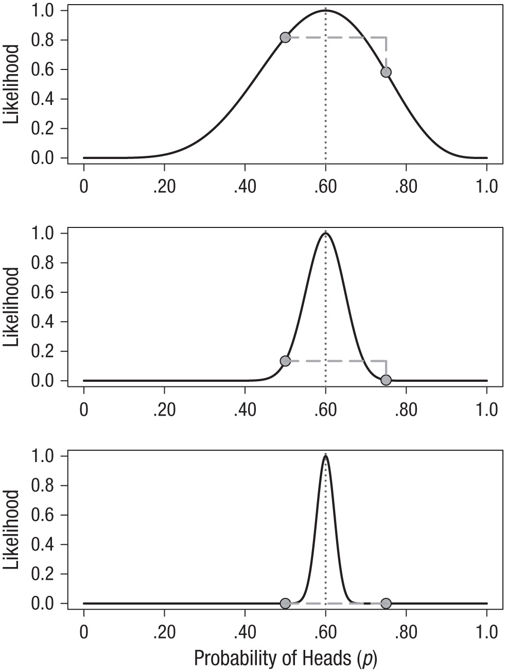
The likelihood functions for observing 6 heads in 10 coin flips (top panel), 60 heads in 100 flips (middle panel), and 300 heads in 500 flips (bottom panel). In each panel, the circles indicate where the fair-coin and trick-coin hypotheses fall on the curve (i.e., hypothesized values of .50 and .75, respectively). The dotted vertical lines indicate the value of p with the greatest likelihood.

The middle panel of Figure 1 shows how the likelihood function changes if instead of tossing the coin 10 times and getting 6 heads, we toss it 100 times and obtain 60 heads: The curve gets much narrower. The strength of evidence favoring the fair-coin hypothesis over the trick-coin hypothesis has also changed; the new likelihood ratio is 29.9. This is much stronger evidence, but because of the narrowing of the likelihood function, neither of these hypothesized values is very high up on the curve any more. It might be more informative to compare each of our hypotheses against the best-supported hypothesis—that the coin is not fair and the probability of heads is .60. This gives us two likelihood ratios: LR(.60,.50) = 7.5 and LR(.60,.75) = 224.

The bottom panel in Figure 1 shows the likelihood function for the case of 300 heads in 500 coin flips. Notice that both the fair-coin and the trick-coin hypotheses appear to be very near the minimum likelihood; yet their likelihood ratio is much stronger than before. For these data, the likelihood ratio comparing these two hypotheses, LR(.50,.75), is 23,912,304, or nearly 24 million. The inherent relativity of evidence is made clear in this example: The fair-coin hypothesis is supported when compared with one particular trick-coin hypothesis. But this should not be interpreted as absolute evidence for the fair coin; the maximally supported hypothesis is still that the probability of heads is .60, and the likelihood ratio for this hypothesis versus the fair-coin hypothesis, LR(.60,.50), is nearly 24,000.

We need to be careful not to make blanket statements about absolute support, such as claiming that the hypothesis with the greatest likelihood is “strongly supported by the data.” Always ask what the comparison is with. The best-supported hypothesis will usually be only weakly supported against any hypothesis positing a value that is a little smaller or a little larger.³ For example, in the case of 60 heads in 100 flips, the likelihood ratio comparing the hypotheses that p = .60 and p = .75 is very large, LR(.60,.75) = 224, whereas the likelihood ratio comparing the hypotheses that p = .60 and p = .65 is much smaller, LR(.60,.65) = 1.7, and provides barely any support one way or the other. Consider the following common real-world research scenario: We have run a study with a relatively small sample size, and the estimate of the effect of primary scientific interest is considered “large” by some criteria (e.g., Cohen’s d > 0.75). We may find that the estimated effect size from the sample has a relatively large likelihood ratio compared with a hypothetical null value (i.e., a ratio large enough to “reject the null hypothesis”; see the next section), but that the likelihood ratio is much smaller when the comparison is with a “medium” or even “small” effect size. Without relatively large sample sizes, one is often precluded from saying anything precise about the size of the effect because the likelihood function is not very peaked when samples are small.

Maximum likelihood estimation

A natural question for a researcher to ask is, what is the hypothesis that is most supported by the data? This question is answered by using a method called maximum likelihood estimation (Fisher, 1922; see also Ly, Marsman, Verhagen, Grasman, & Wagenmakers, 2017, and Myung, 2003). In the plots in Figure 1, the vertical dotted lines mark the value of p that has the highest likelihood; this value is known as the maximum likelihood estimate. We interpret this value of p as being the value that makes the observed data the most probable. Because the likelihood is proportional to the probability of the data given the hypothesis, the hypothesis that maximizes P(D|H) will also maximize L(H). In the case of simple problems, plotting the likelihood function will reveal an obvious maximum. For example, the maximum of the binomial likelihood function will be located at the proportion of successes observed in the sample. Box 1 shows this to be true using a little bit of elementary calculus.⁴

Box 1.

Deriving the Maximum Likelihood Estimate for a Binomial Parameter

The binomial likelihood function is given in Equation 1, and our goal is to find the value of p that makes the probability of the outcome x the largest. Recall that to find possible maximums or minimums of a function, one takes the derivative of the function, sets it equal to 0, and solves. We can find the maximum of the likelihood function by first taking the logarithm of the function and then taking the derivative, because maximizing log[f (y)] will also maximize f (y). Taking the logarithm of the function will make our task easier, as it changes multiplication to addition and the derivative of log[y] is simply 1/y. Moreover, because log-likelihood functions are generally unimodal concave functions (they have a single peak and open downward), if we can do this calculus and solve our equation, then we will have found our desired maximum.

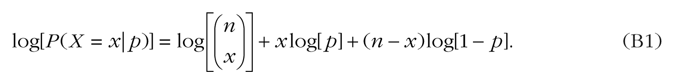
We begin by taking the logarithm of Equation 1:

\log [P (X = x | p)] = \log [(\begin{matrix} n \\ x \end{matrix})] + \log [p^{x}] + \log [{(1 - p)}^{n - x}] .

Remembering the rules of logarithms and exponents, we can rewrite this as

\log [P (X = x | p)] = \log [(\begin{matrix} n \\ x \end{matrix})] + x \log [p] + (n - x) \log [1 - p] .

Now we can take the derivative of Equation B1 as follows:

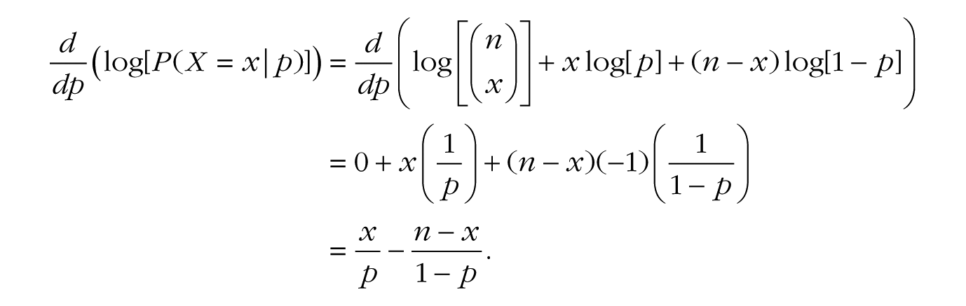
\begin{matrix} \frac{d}{d p} (\log [P (X = x | p)]) = \frac{d}{d p} (\log [(\begin{matrix} n \\ x \end{matrix})] + x \log [p] + (n - x) \log [1 - p]) \\ = 0 + x (\frac{1}{p}) + (n - x) (- 1) (\frac{1}{1 - p}) \\ = \frac{x}{p} - \frac{n - x}{1 - p} . \end{matrix}

(where the –1 in the last term of the second line comes from using the chain rule of derivatives on log[1 – p]). Now we can set the final expression equal to zero, and a few algebraic steps will lead us to the solution for p:

0 = \frac{x}{p} - \frac{n - x}{1 - p}

\frac{n - x}{1 - p} = \frac{x}{p}

n p - x p = x - x p

n p = x

p = \frac{x}{n} .

In other words, the maximum of the binomial likelihood function is found at the sample proportion, namely, the number of successes x divided by the total number of trials n.

With the maximum likelihood estimate in hand, there are a few possible ways to proceed with classical inference. First, one can perform a likelihood ratio test comparing two versions of the proposed statistical model: one in which the parameter of interest, θ, is set to a hypothesized null value and one in which the parameter is estimated from the data (the null model is said to be nested within the second model because it is a special case of the second model in which the parameter equals the null value). In practice, this amounts to comparing the value of the likelihood at the maximum likelihood estimate, θ_mle, and the value of the likelihood at the proposed null value, θ_null. Likelihood ratio tests are commonly used to draw inferences with structural equation models. In the case of the binomial coin-toss example from earlier in this Tutorial, we would compare the probability of the data if p were .50 (the fair-coin hypothesis) with the probability of the data given the value of p estimated from the data (the maximum likelihood estimate). In general, it can be shown that when the null hypothesis is true, and as the sample size gets large, twice the logarithm of this likelihood ratio approximately follows a chi-squared distribution with a single degree of freedom (Casella & Berger, 2002, p. 489; Wilks, 1938):

2 \log [\frac{P (X | θ_{mle})}{P (X | θ_{null})}] \dot{~} χ^{2} (1),

where $\dot{~}$ means “is approximately distributed as.” If the value of the quantity on the left-hand side of Equation 2 is large enough (i.e., lies far enough out in the right tail of the chi-squared distribution), such that the p value is lower than a prespecified cutoff α (often chosen to be .05), then one would make the decision to reject the hypothesized null value.⁵

Second, one can perform a Wald test, in which the maximum likelihood estimate is compared with a hypothesized null value, and this difference is divided by the estimated standard error of the maximum likelihood estimate. Essentially, this test determines how many standard errors separate the null value and the maximum likelihood estimate. The t test and z test are arguably the most common examples of the Wald test, and they are used for making inferences about parameters in settings that range from simple comparisons of means to complex multilevel regression models. For many common statistical models, it can be shown (e.g., Casella & Berger, 2002, p. 493) that if the null hypothesis is true, and as the sample size gets large, the Wald-test ratio approximately follows a normal distribution with a mean of 0 and standard deviation of 1,

\frac{θ_{mle} - θ_{null}}{S E (θ_{mle})} \dot{~} N (0, 1) .

As in the case of the likelihood ratio test, if the value of this ratio is large enough, such that the p value is less than the prespecified α, then one would make the decision to reject the hypothesized null value. This large-sample approximation also allows for easy construction of 95% confidence intervals, by computing θ_mle ± 1.96 × SE(θ_mle). It is important to note that these confidence intervals are based on large-sample approximations and therefore can be suboptimal when samples are relatively small (Ghosh, 1979).

Figure 2, which shows the logarithm of the likelihood function (known as the log likelihood) for 60 heads in 100 flips, illustrates the relationship between the two types of tests. The likelihood ratio test looks at the difference in height between the likelihood at its maximum and the likelihood at the null hypothesis, and rejects the null hypothesis if the difference is large enough. In contrast, the Wald test looks at how many standard errors the maximum is from the null value and rejects the null hypothesis if the estimate is sufficiently far away. In other words, the likelihood ratio test evaluates the vertical discrepancy between two values on the likelihood function (y-axis), and the Wald test evaluates the horizontal discrepancy between two values of the parameter (x-axis). As sample size grows very large, the results from these methods converge (Engle, 1984), but in practice, each has its advantages. An advantage of the Wald test is its simplicity when one tests a single parameter at a time; all one needs is a point estimate and its standard error to easily perform hypothesis tests and compute confidence intervals. An advantage of the likelihood ratio test is that it is easily extended to simultaneously test multiple parameters—by increasing the degrees of freedom of the chi-squared distribution in Equation 2 to be equal to the number of parameters being tested (the Wald test can be extended to the multiparameter case, but it is not as elegant as the likelihood ratio test in such scenarios).

Fig. 2.

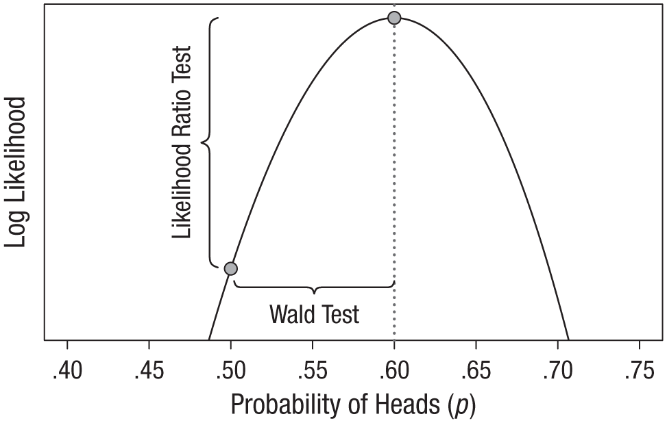
Illustration of the difference between the likelihood ratio test and the Wald test. In this plot of the logarithm of the binomial likelihood function for observing 60 heads in 100 coin flips, the x-axis is restricted to the values of p that have appreciable log-likelihood values. Both tests compare two hypothesized values of p (indicated by the plotted points): the null value, .50, and the maximum likelihood estimate, .60. However, the likelihood ratio test evaluates the points’ vertical discrepancy, whereas the Wald test evaluates their horizontal discrepancy.

Bayesian updating via the likelihood

As we have seen, likelihoods form the basis for much of classical statistics via the method of maximum likelihood estimation. Likelihoods are also a key component of Bayesian inference. The Bayesian approach to statistics is fundamentally about making use of all available information when drawing inferences in the face of uncertainty. This information may be the results from previous studies, newly collected data, or, as is usually the case, both. Bayesian inference allows one to synthesize these two forms of information to make the best possible inference.

Previous information is quantified using what is known as a prior distribution. The prior distribution of θ, the parameter of interest, is P(θ); this is a function that specifies which values of θ are more or less likely, given one’s interpretation of previous relevant information. The information gained from new data is represented by the likelihood function, proportional to P(D|θ), which is then multiplied by the prior distribution (and rescaled) to yield the posterior distribution, P(θ|D), which is then used as the basis for the desired inference. Thus, the likelihood function is used to update the prior distribution to a posterior distribution. Interested readers can find a detailed technical introduction to Bayesian inference in Etz and Vandekerckhove (2017) and an annotated list of useful Bayesian-statistics references in Etz, Gronau, Dablander, Edelsbrunner, and Baribault (2017).

Mathematically, a well-known conditional-probability theorem (first shown by Bayes, 1763) states that the procedure for obtaining the posterior distribution of θ is as follows:

P (θ | D) = K \times P (θ) \times P (D | θ) .

In this context, K is merely a rescaling constant and is equal to 1/P(D). We often write this theorem more simply as

P (θ | D) \propto P (θ) \times P (D | θ),

where ∝ means “is proportional to.”

The following example shows how to use the likelihood function to update a prior distribution into a posterior distribution. The simplest way to illustrate how likelihoods act as an updating factor is to use conjugate distribution families (Raiffa & Schlaifer, 1961). A prior distribution and likelihood function are said to be conjugate when multiplying them together and rescaling results in a posterior distribution in the same family as the prior distribution. For example, if one has binomial data, one can use a beta prior distribution to obtain a beta posterior distribution (see Box 2). Conjugate prior distributions are by no means required for doing Bayesian updating, but they reduce the mathematics involved and so are ideal for illustrative purposes.

Box 2.

Deriving the Posterior Distribution for a Binomial Parameter Using a Beta Prior

Conjugate distributions are convenient in that they reduce Bayesian updating to some simple algebra. We begin with the formula for the binomial likelihood function,

Likelihood \propto p^{x} {(1 - p)}^{n - x}

(notice that the leading term is dropped), and then multiply it by the formula for the beta prior with a and b shape parameters,

Prior \propto p^{a - 1} {(1 - p)}^{b - 1},

to obtain the following formula for the posterior distribution:

Posterior \propto \underset{Prior}{\underset{︸}{p^{a - 1} {(1 - p)}^{b - 1}}} \times \underset{Likelihood}{\underset{︸}{p^{x} {(1 - p)}^{n - x}}} .

The terms in Equation B2 can be regrouped as follows:

Posterior \propto \underset{Successes}{\underset{︸}{p^{a - 1} p^{x}}} \times \underset{Failures}{\underset{︸}{{(1 - p)}^{b - 1} {(1 - p)}^{n - x}}},

which suggests that we can interpret the information contained in the prior as adding a certain amount of previous data (i.e., a – 1 past successes and b – 1 past failures) to the data from our current experiment. Because we are multiplying together terms with the same base, the exponents can be added together in a final simplification step:

Posterior \propto p^{x + a - 1} {(1 - p)}^{n - x + b - 1} .

This final formula looks like our original beta distribution but with new shape parameters equal to x + a and n – x + b. In other words, we started with the prior distribution beta(a,b) and added the successes from the data, x, to a and the failures, n – x, to b, and our posterior distribution is a beta(x + a,n – x + b) distribution.

Consider the previous example of observing 60 heads in 100 flips of a coin. Imagine that going into this experiment, we had some reason to believe the coin’s bias was within .20 of being fair in either direction; that is, we believed that p was likely within the range of .30 to .70. We could choose to represent this information using the beta(25,25) distribution⁶ shown as the dotted line in Figure 3. The likelihood function for the 60 flips is shown as the dot-and-dashed line and is identical to that shown in the middle panel in Figure 1. Using the result from Box 2, we know that the resulting posterior distribution for p is a beta(85,65) distribution, shown as the solid line in Figure 3.

Fig. 3.

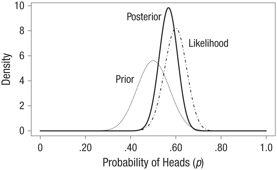
Illustration of Bayesian updating of a prior distribution to a posterior distribution. In this example of a coin-flip experiment, the prior distribution reflects the expectation that the coin is within .20 of being fair in either direction, and the likelihood function is based on the observation of 60 heads in 100 flips. The posterior distribution is a compromise between the information brought by those two distributions.

The entire posterior distribution represents the solution to our Bayesian estimation problem, but researchers often report summary measures to simplify the communication of results. For instance, we could point to the maximum of the posterior distribution—known as the maximum a posteriori estimate—as our best guess for the value of p, which in this case is .568. Notice that this is slightly different from the maximum likelihood estimate, .60. This discrepancy is due to the extra information about p provided by the prior distribution; as shown in Box 2, the prior distribution effectively adds a number of previous successes and failures to our sample data. Thus, the posterior distribution represents a compromise between the information we had regarding p before the experiment and the information gained about p by doing the experiment. Because we had previous information suggesting that p is probably close to .50, our posterior estimate is said to be “shrunk” toward .50. Bayesian estimates tend to be more accurate and to lead to better empirical predictions than the maximum likelihood estimate in many scenarios (Efron & Morris, 1977), especially when the sample size is relatively small.

Likelihood also forms the basis of the Bayes factor, a tool for conducting Bayesian hypothesis tests first proposed by Wrinch and Jeffreys (Jeffreys, 1935; Wrinch & Jeffreys, 1921) and independently developed by Haldane (Haldane, 1932; although see Etz & Wagenmakers, 2017). An important advantage of the Bayes factor is that it can be used to compare any two models regardless of their form, whereas the frequentist likelihood ratio test can compare only two hypotheses that are nested. Nevertheless, when nested hypotheses are compared, Bayes factors can be seen as simple extensions of likelihood ratios. In contrast to the frequentist likelihood ratio test outlined earlier, which evaluates the size of the likelihood ratio comparing θ_null to θ_mle, the Bayes factor takes a weighted average of the likelihood ratio across all possible values of θ; the likelihood ratio is evaluated at each value of θ and weighted by the prior probability density assigned to that value, and then these products are added up to obtain the Bayes factor (mathematically, this is done by integrating the likelihood ratio with respect to the prior distribution; see the appendix).

Conclusion

This Tutorial has defined likelihood, shown what a likelihood function looks like, and explained how this function forms the basis of two common inferential procedures: maximum likelihood estimation and Bayesian inference. The examples used were intentionally simple and artificial to keep the mathematical burden light, but I hope that they can give some insight into the fundamental statistical concept known as likelihood.

Footnotes

Appendix

Note that for a generic random variable ω, the expected value (i.e., average) of the function g(ω) with respect to a probability distribution P(ω) is defined as

E_{ω} [g (ω)] = \int_{Ω} g (ω) P (ω) d ω .

I use this definition of expected value to show that the Bayes factor for a comparison of nested models can be written as the expected value of the likelihood ratio with respect to the specified prior distribution.

The Bayes factor comparing H₁ with H₀ is written similarly to the likelihood ratio:

B F_{10} = \frac{P (D | H_{1})}{P (D | H_{0})} .

In the context of comparing nested models, H₀ specifies that θ = θ_null, so P(D|H₀) = P(D|θ_null); H₁ assigns θ a prior distribution, θ ~ P(θ), so that $P (D | H_{1}) = \int_{Θ} P (D | θ) P (θ) d θ$ . Thus, we can rewrite Equation A1 as

B F_{10} = \frac{\int_{Θ} P (D | θ) P (θ) d θ}{P (D | θ_{null})} .

Because the denominator of Equation A2 is a fixed number, we can bring it inside the integral, and we can see that the resulting expression has the form of the expected value of the likelihood ratio between θ and θ_null with respect to the prior distribution of θ:

\begin{array}{l} B F_{10} = \int_{Θ} \overset{L R (θ, θ_{null})}{\overset{︷}{\frac{P (D | θ)}{P (D | θ_{null})}}} P (θ) d θ \\ = E_{θ} [L R (θ, θ_{null})] . \end{array}

Acknowledgements

A portion of this material previously appeared on my personal blog (). I am very grateful to Quentin Gronau and J. P. de Ruiter for helpful comments.

Action Editor

Daniel J. Simons served as action editor for this article.

Author Contributions

A. Etz is the sole author of this article and is responsible for its content.

ORCID iD

Alexander Etz

Declaration of Conflicting Interests

The author(s) declared that there were no conflicts of interest with respect to the authorship or the publication of this article.

Funding

The author was supported by Grant 1534472 from the National Science Foundation’s Methods, Measurements, and Statistics panel, as well as by the National Science Foundation Graduate Research Fellowship Program (Grant DGE1321846).

Notes

References

Bayes

(1763). An essay towards solving a problem in the doctrine of chances. By the late Rev. Mr. Bayes, F. R. S. Communicated by Mr. Price, in a letter to John Canton, A. M. F. R. S. Philosophical Transactions, 53, 370–418.

Birnbaum

(1962). On the foundations of statistical inference [Target article and discussion]. Journal of the American Statistical Association, 57, 269–326.

Casella

Berger

R. L.

(2002). Statistical inference (Vol. 2). Pacific Grove, CA: Duxbury.

Edwards

A. W. F.

(1974). The history of likelihood. International Statistical Review/Revue Internationale de Statistique, 42, 9–15.

Edwards

A. W. F.

(1992). Likelihood. Baltimore, MD: Johns Hopkins University Press.

Efron

Morris

(1977). Stein’s paradox in statistics. Scientific American, 236, 119–127.

Engle

R. F.

(1984). Wald, likelihood ratio, and Lagrange multiplier tests in econometrics. In Griliches

Intriligator

M. D.

(Eds.) Handbook of Econometrics (Vol. 2, pp. 775–826). Amsterdam, The Netherlands: Elsevier Science.

Etz

Gronau

Q. F.

Dablander

Edelsbrunner

P. A.

Baribault

(2017). How to become a Bayesian in eight easy steps: An annotated reading list. Psychonomic Bulletin & Review. Advance online publication. doi:10.3758/s13423-017-1317-5

Etz

Vandekerckhove

(2017). Introduction to Bayesian inference for psychology. Psychonomic Bulletin & Review. Advance online publication. doi:10.3758/s13423-017-1262-3

10.

Etz

Wagenmakers

E.-J.

(2017). J. B. S. Haldane’s contribution to the Bayes factor hypothesis test. Statistical Science, 32, 313–329.

11.

Fisher

R. A.

(1922). On the mathematical foundations of theoretical statistics. Philosophical Transactions of the Royal Society of London A: Containing Papers of a Mathematical or Physical Character, 222, 309–368.

12.

Ghosh

(1979). A comparison of some approximate confidence intervals for the binomial parameter. Journal of the American Statistical Association, 74, 894–900.

13.

Gronau

Q. F.

Wagenmakers

E.-J.

(in press). Bayesian evidence accumulation in experimental mathematics: A case study of four irrational numbers. Experimental Mathematics.

14.

Haldane

J. B. S.

(1932). A note on inverse probability. Mathematical Proceedings of the Cambridge Philosophical Society, 28, 55–61.

15.

Jeffreys

(1935). Some tests of significance, treated by the theory of probability. Mathematical Proceedings of the Cambridge Philosophical Society, 31, 203–222.

16.

Lindley

D. V.

(1993). The analysis of experimental data: The appreciation of tea and wine. Teaching Statistics, 15, 22–25.

17.

Marsman

Verhagen

Grasman

R. P. P. P.

Wagenmakers

E.-J.

(2017). A tutorial on Fisher information. Journal of Mathematical Psychology, 80, 40–55.

18.

Myung

I. J.

(2003). Tutorial on maximum likelihood estimation. Journal of Mathematical Psychology, 47, 90–100.

19.

Pawitan

(2001). In all likelihood: Statistical modelling and inference using likelihood. Oxford, England: Oxford University Press.

20.

Raiffa

Schlaifer

(1961). Applied statistical decision theory. Cambridge, MA: MIT Press.

21.

Rouder

J. N.

(2014). Optional stopping: No problem for Bayesians. Psychonomic Bulletin & Review, 21, 301–308.

22.

Royall

R. M.

(1997). Statistical evidence: A likelihood paradigm. London, England: Chapman & Hall.

23.

Wilks

S. S.

(1938). The large-sample distribution of the likelihood ratio for testing composite hypotheses. The Annals of Mathematical Statistics, 9, 60–62.

24.

Wrinch

Jeffreys

(1921). On certain fundamental principles of scientific inquiry. Philosophical Magazine, 42, 369–390.

Introduction to the Concept of Likelihood and Its Applications

Abstract

Keywords

The Likelihood Axiom

Likelihoods Are Meant to Be Compared

Inference Using the Likelihood Function

Visual inspection

Maximum likelihood estimation

Deriving the Maximum Likelihood Estimate for a Binomial Parameter

Bayesian updating via the likelihood

Deriving the Posterior Distribution for a Binomial Parameter Using a Beta Prior

Conclusion

Footnotes

Appendix

Acknowledgements

Action Editor

Author Contributions

ORCID iD

Declaration of Conflicting Interests

Funding

Notes

References