Sage Journals: Discover world-class research

Abstract

Path models to test claims about mediation and moderation are a staple of psychology. But applied researchers may sometimes not understand the underlying causal inference problems and thus endorse conclusions that rest on unrealistic assumptions. In this article, we aim to provide a clear explanation for the limited conditions under which standard procedures for mediation and moderation analysis can succeed. We discuss why reversing arrows or comparing model fit indices cannot tell us which model is the right one and how tests of conditional independence can at least tell us where our model goes wrong. Causal modeling practices in psychology are far from optimal but may be kept alive by domain norms that demand every article makes some novel claim about processes and boundary conditions. We end with a vision for a different research culture in which causal inference is pursued in a much slower, more deliberate, and collaborative manner.

Keywords

causal modeling structural equation modeling SEM mediation moderation

Psychologists often do not content themselves with claims about the mere existence of effects. Instead, they strive for an understanding of the underlying processes and potential boundary conditions. Although such models are frequently estimated with the help of structural equation models (SEM), the PROCESS macro (Hayes, 2017) has been an extraordinarily popular tool for these purposes because it empowers users to run mediation and moderation analyses—and any combination of the two—with a large number of preprogrammed model templates in a familiar software environment.

Psychologists’ enthusiasm for models that allow them to unravel mediation, moderation, and their combination may sometimes lead them to overlook the many assumptions that are necessary to interpret results. Although it is clear that correlation does not equal causation, it is not immediately obvious how this translates to more complex models fitted to (mostly) observational data, in which not all causes of interest were experimentally manipulated. Analyses may result in seemingly sophisticated conclusions that are ultimately unwarranted.¹

With this article, we aim to provide a concise summary of the causal-inference problems of path models that incorporate mediation and moderation. “Causal inference” refers to any attempt to use empirical data to make conclusions about causal effects, and causal effects imply that a (hypothetical) intervention on one variable leads to a change in a different variable, for at least some people. We start with a so-called conditional-process model, which combines mediation and moderation, and work our way back to the underlying assumptions. We provide nontechnical explanations so that readers can develop an intuition for the intricacies of such path models. We then discuss matters of model selection—How can we know that we got the model right?—and conclude with our vision for a different research process that results in better causal claims. Ultimately, as a field, we do indeed want to understand processes and boundary conditions. But a single study, let alone a single statistical analysis, can rarely provide a satisfying answer.

The Conditional-Process Model

Consider the conceptual diagram in Figure 1. It depicts a path model in which an independent variable has an effect on a dependent variable via a mediator and one of the mediation paths is moderated.² For example, researchers may hypothesize that social support has an effect on task performance among athletes. Supposedly, this effect is partly mediated via self-efficacy: Social support leads athletes to believe in themselves, and this improves performance. But this mediation may apply only to highly stressed athletes. Among more relaxed athletes, social support may not be a salient source of self-efficacy. By convention, such conceptual diagrams usually imply linear relationships between the variables. We adapted this substantive illustration from Rees and Freeman (2009); it was also highlighted in Hayes (2017).

Fig. 1.

A conceptual diagram of a conditional-process model in which a mediated path is affected by a moderator.

When we test such hypotheses with the help of path models applied to observational data, we are in the business of causal inference on the basis of observational data (for an introduction, see e.g., Rohrer, 2018). One may object that such path models are employed for other purposes, such as description or prediction. However, the models may be too complex to result in useful description (for a similar argument, see Foster, 2010b), and they are not complex and flexible enough to result in useful prediction (for an introduction to machine learning, see Westfall & Yarkoni, 2016). Furthermore, reviews of path models in different literatures from the social and behavioral sciences have concluded that causal inferences are made or implied routinely (e.g., Fiedler et al., 2018; Wood et al., 2008). And it only makes sense to talk about and interpret mediation from a causal perspective; from a strictly statistical perspective, the phenomenon is indistinguishable from confounding (MacKinnon et al., 2000).

In the field of psychology, causal inference on the basis of observational data is treated with some degree of suspicion because the field tends to emphasize randomized experiments as the “gold standard.” There is indeed a lot that speaks in favor of experiments and other predominantly design-based approaches to causal inference (i.e., natural experiments; e.g., Dunning, 2012). However, once we have settled on a model such as the one depicted in Figure 1, or in general once we are interested in mediation, our approach will necessarily be more strongly model-based. We believe that to make the most of causal inference on the basis of observational data, it is best to take the bull by the horns while remaining transparent about the underlying assumptions rather than resorting to ambiguous language that obscures the goal of the analysis (Grosz et al., 2020). Indeed, explicit causal language may prompt readers to be more careful when they evaluate whether conclusions are appropriate (Alvarez-Vargas et al., 2020).

Under what conditions can we fit the model depicted in Figure 1 and successfully interpret the resulting coefficients as causal effects? The central concern here is causal identification (Elwert, 2013), which refers to the possibility of computing accurate causal effects from observable data, and which is the focus of this article. However, we also address the second step of causal inference, actual statistical estimation. Causal identification always rests on assumptions, and existing formalized frameworks allow for precise articulation of the underlying assumptions (e.g., directed acyclic graphs, the Rubin causal model; for a helpful introduction, see Morgan & Winship, 2015). Here, we use a more informal approach—starting from a single arrow and moving on to more complex claims about mediation and moderation. Many of the assumptions that go into the model are irrefutable; they cannot be disproved (let alone proved) by observable information (Manski, 2009). Throughout the article, we often focus on concerns regarding how conditional-process models are commonly implemented and interpreted in psychology. Although there is now a number of studies that have empirically investigated such practices (see Box 1), our assessment of what is common practice is at least partly formed according to our own reading of the literature and thus somewhat subjective.

Box 1.

Conditional Process Models as Practiced in Psychology

Common practices in the application of conditional-process models for causal inference in psychological research, or any field, are somewhat difficult to study empirically because we are limited to details disclosed in publications, which may not always diligently report the process by which such models have been generated. Such reporting can obscure relevant information, and in many cases, it is impossible to evaluate whether the researchers actually believe the assumptions that underlie their reported models.
The comprehensive database by Fossum and Montoya (2021) documents basic practices in moderated mediation models, such as the estimation procedure, sample size, model number according to Hayes’s (2017) typology, and number of variables, across a wide spectrum of research areas. The study by Götz et al. (2021) is concerned with practices in such mediation models that are questionable and contrasted the statistical power with the hypothesis confirmation rate in five leading psychology journals in 2018 and 2019. Likewise, Fiedler et al. (2018) observed that in a sample of articles published in 2015, only a minority of them with mediation analyses even present a priori theoretical arguments for the proposed causal chain in the first place.

An arrow is an arrow is an arrow

One can determine the assumptions under which such a model successfully identifies the causal effects by considering every single arrow it contains. For example, let us start with the arrow pointing from the independent variable to the mediator, Social Support → Self-Efficacy. This single-headed arrow represents a causal effect of social support on self-efficacy. In general, a variable X has a causal effect on Y if a (hypothetical) intervention on X leads to a change in Y for at least one individual. Assuming linear effects, in psychology, we often try to estimate how a given change in X (e.g., an increase of 1 scale point) would affect Y, on average. If we want to be able to quantify the causal effect of social support on self-efficacy and to put the correct number on this arrow, we need to rule out (a) confounding and (b) reverse causality.

Confounding

To rule out confounding, we need to ensure that any possible variable that causally affects both social support and self-efficacy is taken into account (see Fig. 2a for an example of one potential confounder: extraversion). This can, for example, be done by including it as a covariate. To successfully control for confounding, it is important that the association with the covariate is modeled appropriately (i.e., if the effect of the covariate is nonlinear, it needs to be modeled nonlinearly; see also Rohrer, 2018), and it may be necessary to take into account measurement error in the covariate (Westfall & Yarkoni, 2016). For example, imagine the following situation: More extraverted individuals receive more social support, and they tend to score higher on self-efficacy. Thus, if we do not adjust for extraversion, we will overestimate the effect of social support on self-efficacy. However, imagine our measure of extraversion was quite imprecise—for example, we may have just asked individuals to say whether they are extraverted (yes/no). If we adjust for this unreliable measure, there is still plenty of extraversion-associated variability left. Among the people who say they are extraverted, there will still be some who are more extraverted than others and who thus score higher on both social support and self-efficacy. In this situation, statistical adjustment may end up insufficient and leave residual confounding that can lead us to still overestimate the actual effect of social support on self-efficacy.

Fig. 2.

Modifications of the conditional-process model from Figure 1. (a) A confounder between independent variable and mediator will bias the estimated path. (b) If we can intervene on the independent variable, the confounder is no longer a problem and we can estimate the causal effects of the independent variable on other variables.

Including all possible confounders seems like a daunting task, and in some scenarios, things can be simplified. For example, sometimes a single covariate can take care of multiple confounding variables (for an introduction on how to determine whether a set of covariates is sufficient, see Rohrer, 2018); in longitudinal data or otherwise nested data, fixed effects can account for a multitude of confounders, including unobserved ones (e.g., Imai & Kim, 2019; Rohrer & Murayama, 2021).

Reverse causality

Temporal order can sometimes rule out reverse causality. Tomorrow’s self-efficacy cannot have a causal effect on today’s social support. But note that temporal order cannot rule out confounding. If yesterday’s self-efficacy had a causal effect on today’s social support and an effect on tomorrow’s self-efficacy, this would result in a spurious association between today’s social support and tomorrow’s self-efficacy (i.e., yesterday’s self-efficacy is a confounder). In other cases, substantive knowledge may help rule out reverse causality, in particular if stable demographic variables are involved.

The value of randomized manipulation

One way to rule out both confounding and reverse causality is an experimental manipulation of the independent variable with subsequent measurement of any dependent variable. For example, we could randomly assign athletes to receive high or low social support before an event and then later measure their self-efficacy and their task performance. Figure 2b provides a graphical interpretation of such an intervention: Any path that points into the independent variable is deleted because randomly assigned social support is determined by chance (e.g., the flip of a coin) only.³ Such an experimental manipulation allows a causal interpretation of the total effect of the manipulation on any outcome; for example, we could make causal claims about how our social-support manipulation affects self-efficacy or about how it affects task performance.

Unfortunately, being able to identify the total effect of one variable on another does not mean that we can automatically identify path-specific effects (for technical details on such effects, see Avin et al., 2005), such as indirect or direct effects. This leads us to problems of mediation analysis.

Mediation: double trouble

Identification of the indirect effect

Claims about mediation, within the “causal chain” approach of path models that dominates psychology, are claims about the product of two causal effects. For example, the indirect effect of social support on task performance via self-efficacy (Social Support → Self-Efficacy → Task Performance) would be the causal effect of social support on self-efficacy combined with the causal effect of self-efficacy on task performance. Thus, we must be able to identify two causal effects to identify an indirect effect. If either of the two estimates is confounded, the estimate of the indirect effect will be confounded as well. In addition, we need to assume that both effects are linear and that the independent variable does not interact with the mediator (i.e., that the effect of social support does not change depending on the level of self-efficacy)—unless we modify our model to account for such scenarios.

These are quite strong assumptions. Even in standard experimental designs, problems arise when the mediator has not been randomized (e.g., Bullock et al., 2010). For example, even if we were able to randomize social support, our estimate of the effect of self-efficacy on task performance would still deviate from the actual causal effect unless we assumed that we controlled for all common causes of these two variables (i.e., no unmeasured confounding; for an example of a confounder, see Fig. 3a) and unless we assumed that there was no reverse causality.

Fig. 3.

More modifications of the conditional-process model. (a) A confounder between mediator and the dependent variable will bias the estimate of the indirect effect. Furthermore, statistical control for the mediator will induce a spurious association between the confounder and the independent variable (indicated by the dashed line), which will bias the estimate of the direct effect. (b) A moderator may be confounded and thus not the variable that actually causally interacts with the independent variable.

Identification of the direct effect

Readers may recall that the total effect equals the sum of the indirect effect plus the direct effect, which is true under certain assumptions (if all causal effects are linear and do not vary between individuals). Could that help us identify the indirect effect? After all, we noted above that with the help of randomization, we can identify the total effect of social support on task performance. If we additionally knew the direct effect, we could simply calculate the indirect effect as the difference between the two. The standard procedure for estimating the direct effect is statistical adjustment for the mediator, which is meant to “shut off” the indirect path and thus leave only the direct path. Unfortunately, this does not work here. The mediator (self-efficacy) is causally affected by social support and other factors; it is a “collider” in which the effects of multiple variables come together. If we statistically adjust for a collider variable, we introduce spurious associations between its causes (Elwert & Winship, 2014; for more explanation geared toward psychologists, see also Rohrer, 2018). For example, here, conditioning on self-efficacy may introduce a spurious association between social support and previous task performance (Fig. 3a).⁴ Previous task performance affects current task performance, and so we have actually introduced an additional spurious association: Social support is now confounded with previous task performance, which affects current task performance. Thus, we cannot give a causal interpretation to the coefficient of the direct effect of social support on task performance. We may fix this issue by statistically adjusting for previous task performance and any other variable that affects both self-efficacy and task performance, which leads us back to the strong assumptions that we have successfully measured and adjusted for all common causes of the mediator and the dependent variable.

Improving mediation analysis

MacKinnon and Pirlott (2015) summarized some steps that researchers can take to increase the plausibility of mediation claims, such as different ways to adjust for confounders, and sensitivity analyses that probe to which extent estimates are robust to unobserved confounding (developed by Imai et al., 2010; VanderWeele, 2010). Modern causal mediation analysis (e.g., Imai et al., 2010) has moved away from the simple causal chain method that is currently favored in psychology; MacKinnon et al. (2020) explained how the different methods are linked.

Even in the absence of confounders, mediation chains unfold over time, and trying to recover the longitudinal effects from cross-sectional data works only under very narrow conditions (Maxwell & Cole, 2007; Maxwell et al., 2011; O’Laughlin et al., 2018). Thus, in many scenarios, longitudinal data may be needed; these are generally helpful because they can address at least some concerns regarding unobserved confounders (Rohrer & Murayama, 2021). Another idea to improve mediation claims involves chaining them together “piece by piece,” for example, by running multiple experiments. Combining such independent estimates still requires substantial assumptions (e.g., Imai et al., 2011, p. 770), although they may often be more defensible (Pirlott & MacKinnon, 2016; Strobl & Wunsch, 2018). At the same time, this of course presumes that the mediator can be manipulated in a targeted manner, which may not always be the case, in particular if it is a psychological variable (Eronen, 2020).

Compounding Complexities With Multiple Mediators

Here, we have focused on a model with a single mediator. Of course, it is plausible (if not self-evident) that in reality, any causal chain can be broken down into increasingly fine steps (i.e., serial mediators), and any remaining “direct” effect is transmitted via other intermediary variables (i.e., parallel mediators). The mere existence of multiple mediators is not a problem per se—if the crucial assumption of mediation analysis, sequential ignorability,⁵ is fulfilled, we can still identify a particular causal mechanism of interest (Imai et al., 2011). However, certain constellations with multiple mediators make it harder or impossible to achieve sequential ignorability.

The situation depicted in Figure 4 warrants special attention. Here, a second mediator (M2) affects the mediator of interest (M1). If M2 was unobserved, it would be a confounder between both X and M1 and between M1 and Y, which would make it impossible to identify the indirect effect via M1. However, if M2 is observed and if we assume that all effects are linear and the same for everyone, there is no problem: We can identify every single path in the model, and to get the indirect effects, we simply multiply the path coefficients. This breaks down if we leave behind the assumption that all effects are linear and the same for everyone. In this scenario, an interesting asymmetry arises: We can still identify the (average) causal mediation effect of M2 even if M1 was unobserved. However, we can no longer identify the causal mediation effect of M1 even if M2 is observed. That is because M2 is a posttreatment confounder, and the existence of such confounders violates sequential ignorability (see Note 5). The problem is explained in more detail in the appendix of Imai et al. (2011, Figure 8). It highlights two aspects: First, strong (and potentially unrealistic) assumptions about functional form can greatly simplify causal identification; second, whether a second mediator is a problem depends on the specific constellation of mediators—here, M2 is a problem for M1, but M1 is not a problem for M2.

Fig. 4.

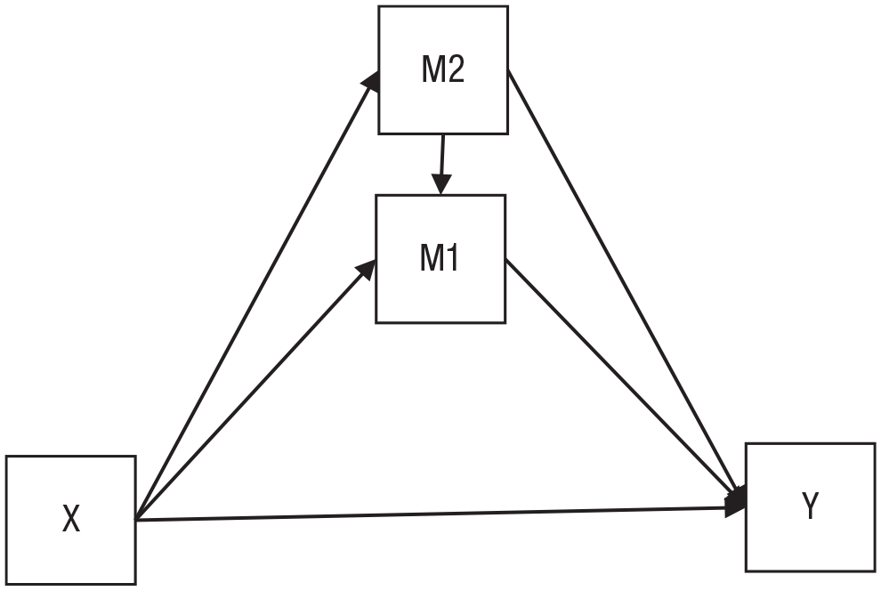
A second mediator acts as a confounder between the first mediator and the outcome. If both effects are linear and homogeneous, we can still identify all indirect effects as long as both mediators are observed. However, if we relax the assumptions about functional form, we can identify only the causal mediation effect of the second mediator (M2).

Everything in moderation: causal interaction versus effect heterogeneity

“Moderation” colloquially refers to a situation in which the effect of one variable on another variable “depends” on the level of a third variable, the moderator. For example, social support may increase self-efficacy, but only among people who experience a lot of stress at home. From a causal-inference perspective, such moderation can refer to two different phenomena.

Causal interaction

An actual causal interaction would imply that a hypothetical intervention on the moderator would causally affect the magnitude of the effect of interest (see e.g., VanderWeele, 2009). For example, if stress indeed causally interacts with social support, then an intervention on stress would change the effects of social support. Such a causal interaction is symmetrical: We may say that higher stress leads to a higher effect of social support on self-efficacy but also that higher social support leads to a higher effect of stress on self-efficacy. To correctly estimate such a causal interaction, we need to be able to properly identify the effect of the moderator. Randomization is once again the most direct way to do this, but in case this is not feasible, covariates may be included to rule out confounders. For example, as depicted in Figure 3b, it may actually be neuroticism that causally interacts with social support, not stress. To rule this out, we would need to statistically adjust for neuroticism. Here, it is important that we also include the interaction between any relevant covariate and the independent variable (Simonsohn, 2019; Yzerbyt et al., 2004)—note that this is unfortunately not standard practice and not the default in most software packages, so it needs to be done manually (e.g., by computing product variables and including them as covariates).

Heterogeneous effects that correlate with a third variable

However, one can also conceive of a type of “noncausal moderation” in which the causal effect is heterogeneous—it varies between individuals—and its magnitude simply correlates with a third variable (e.g., VanderWeele, 2009). Here, an intervention on the third variable would not necessarily result in a larger or smaller effect, and the situation can be asymmetrical: The third variable may correlate with the effect of X on Y, but X need not correlate with the effect of the third variable (which may, in fact, be zero). Such correlations between causal effects and third variables can be expected to change in magnitude, depending on which other covariates are included in the model.

Nonetheless, such noncausal associations between causal effects and third variables may be of interest to researchers. For example, in a clinical setting, one may want to determine subgroups of patients for which a treatment works particularly well. Analyses may indicate that effects are particularly large among individuals with comorbid depression. Even if we do not know whether depression is indeed causally interacting with the treatment or whether instead some confounding factor (e.g., socioeconomic status) causally affects the treatment effects, this information could still be helpful to guide treatment decisions. However, such a valid predictive interpretation may often lead to follow-up questions that require us to clarify the causal role of depression. For example, a clinical researcher may wonder why the treatment works well among depressed individuals: Is the treatment particularly effective against cognitive patterns that are common in depressed patients? Or is it just that the treatment is particularly helpful for individuals who have a low income?

Presenting and interpreting a mere correlation between causal effects and a third variable takes some care to prevent findings from being misread as a causal interaction. For example, a diagram such as Figure 1 should be avoided because the arrow that points away from the third variable begs to be interpreted as a causal interaction. And even just the term “moderator” may be sufficient to induce a causal interpretation because it is usually used to refer to causal interactions. Finally, both causal interactions and correlations between variables and effects can be quite challenging not only because of causal concerns but also because of additional statistical stumbling blocks (e.g., Rohrer & Arslan, 2021).

Finding the Right Model

As we described above, correctly estimating causal effects is challenging, and it always hinges on getting the model right (even in experiments). But how do we know that we have gotten the model right? Researchers may want to evaluate a particular model they have fitted to their data or decide between multiple alternative models. The latter may rarely happen in practice (e.g., Chan et al., 2020) and may often go wrong.

Comparing alternative models

In mediation analysis, researchers sometimes aim to compare alternative mediation hypotheses by switching the direction of arrows (see Fig. 5) and comparing the size and statistical significance of the estimated indirect effects. In particular, the model with the nonzero or larger indirect effect is thought to be supported by the data. Imagine the following scenario: After we run Model A, we find a large indirect effect of X on Y via M. After we run Model B, we find a smaller indirect effect of M via X on Y. The conclusion that Model A is correct because the indirect effect is larger, however, is flawed. Why would we presuppose the existence of a (large) indirect effect if mediation analysis is supposed to tell us whether there is an indirect effect? And the estimate of the indirect effect can be interpreted only if we assume that we got the model right to begin with. A misspecified model may detect a large indirect effect that is entirely spurious.

Fig. 5.

(a) Self-efficacy mediates the effect of social support on task performance. (b) The arrow from social support to self-efficacy has been reversed, so now social support mediates the effect of self-efficacy on task performance. Both models belong to the same equivalence class and are thus statistically indistinguishable.

But if the magnitude of the estimated indirect effects is not informative, maybe at least we can compare the fit of the models to figure out which one is preferable. Unfortunately, reversing arrows results in models that are equally supported by the data at hand; they belong to the same equivalence class. This means that they share the same implied covariance matrix (Thoemmes, 2015); they are observationally equivalent. On a substantive level, these models may look quite different. For example, in Figure 5a, self-efficacy mediates the effects of social support on task performance (and social support confounds the association between self-efficacy and task performance). In Figure 5b, social support mediates the effects of self-efficacy on task performance (and self-efficacy confounds the association between social support and task performance). But no matter which model from the equivalence class we assume to be the actual data-generating process, we will always expect to observe the same empirical associations between the variables. This means that the empirical data alone cannot possibly distinguish between these models, a problem that is well known in the literature on structural modeling (e.g., MacCallum et al., 1993).

Global model fit

Equivalence classes are also the reason why the evaluation of model fit measures (e.g., the mean squared error, R², strictly speaking a measure of predictive performance, or, in a SEM context, χ², root mean square error of approximation, comparative fit index) alone can never tell us whether our model is correct: Each model from an equivalence class will produce identical fit indices. However, considerations of model fit may at least enable us to discard certain models as implausible. If the model appropriately captures the underlying causal data-generating process, model fit will be good—thus, models with a bad fit cannot have generated the data. To actually apply this logic, we need to move analyses into a SEM context in which we can properly assess and compare model fit.

Local misfit

Although global assessments of model fit are most common in psychology, it may often be helpful to additionally apply more local approaches that can tell us why a model does not fit well (Pearl et al., 2016, p. 50). If we assume that a certain causal model generated our data, we can derive testable implications. Testable implications are about the independence of pairs of variables—casually speaking, the fewer arrows between variables, the more things we can test. Testable implications take the form of “adjusting for C, A and B are statistically independent”—if this is not the case in our empirical data, we can reject the assumed model, and we also know where it went wrong (e.g., we missed a factor that causes an association between A and B). The directed acyclic graph framework provides clear rules for how to derive all testable implications of a given model (Elwert, 2013, pp. 252–254; Pearl et al., 2016, Chapter 2.5), and there is even software that automates the process (e.g., dagitty.net; see also Textor et al., 2011). In Box 2, we give a brief introduction on how to derive testable implications. Models from the same equivalence class share the same testable implications and thus firmly remain empirically indistinguishable. Furthermore, note that some process models do not have testable implications because they are saturated: The model has so many parameters that it can perfectly reproduce the empirically observed associations; in a SEM context, model fit would necessarily be perfect (with zero degrees of freedom)—the model thus cannot possibly fail, and no testable implications remain.

Box 2.

Spotlight on Testable Implications

To derive testable implications, we can break up a causal graph into three elementary causal structures (Elwert, 2013) that do (or do not) transmit associations between variables.
Chains: A → B → C. This chain transmits a causal association between A and C. If we control for the third variable (B, the mediator), the chain ceases to transmit an association. Considering this chain in isolation, this means that conditional on B, A and C are independent, which we can write as A ⊥ C | B.
Forks: A ← C → B. This fork transmits a noncausal association between A and B. If we control for the third variable (C, the confounder), the fork ceases to transmit an association: A ⊥ B | C.
Inverted fork: A → C ← B. This inverted fork does not transmit an association between A and B, A ⊥ B. However, if we control for the third variable (C, the collider), then the inverted fork transmits a noncausal association between A and B.
We can break up all paths in Figure 3a into these elementary structures to arrive at the testable implications of the model. Note that here, we will assume that the graph fully represents the assumed model, which is generally not the case for such conceptual graphs (more on that below).
Some variables should not be associated in the overall data:
Past Performance ⊥ Social Support
Past Performance ⊥ Stress
Social Support ⊥ Stress.
Furthermore, task performance and stress should not be associated when we control for past performance, self-efficacy, and social support:
Task Performance ⊥ Stress | Past Performance, Self-Efficacy, Social Support.
However, if we specify this particular model in PROCESS and most other software, per default, variables that jointly cause another variable are allowed to correlate (unless one of them causes the other). This means that in many conceptual graphs, there are a number of bidirectional arrows that are not depicted (Hayes, 2017, p. 22) and that reduce the number of testable implications. As a result, many of the models implemented in the PROCESS macro are observationally equivalent. According to our analysis (see https://osf.io/69kgc/), of the 58 models included in the current version, 86% are equivalent to at least one other model. Overall, the 58 models belong to only 17 different equivalence classes.
If we include these additional arrows and once again deduce all testable implications for our central example, we are left with only one of them:
Task Performance ⊥ Stress | Past Performance, Self-Efficacy, Social Support.
What if we find that task performance and stress are still correlated after adjusting for past performance, self-efficacy, and social support? We may reject the underlying substantive model or modify it. For example, it is possible that conditional independence is violated only because of measurement error in past performance, self-efficacy, or social support, which could be explicitly incorporated into the graph (Kuroki & Pearl, 2014).

Model equivalence when mediation is moderated

Earlier, we stated that switching the direction of arrows in mediation models results in observationally equivalent models. But does that also apply to moderated mediation? To find out, we can draw a moderated mediation model, apply the rules described in Box 2 to derive testable implications, then switch some arrows, and check whether the testable implications have changed. If models have different testable implications, they are no longer observationally equivalent, and empirical data may lead us to reject some but not all possible moderated mediation models. Of course, whether a moderated mediation model that cannot be rejected by the data actually depicts a plausible causal net still depends on additional assumptions (e.g., the absence of unobserved confounders discussed above). In Figure 6, we demonstrate what this exercise of repeatedly deriving testable implications would look like for a scenario in which a moderator affects only one mediation path and in which any correlation between the moderator and the respective independent variable is due to an unobserved common cause.⁶ We can see that once the moderator is added, only some models remain observationally equivalent.

Fig. 6.

Testable implications of different moderated mediation models. Z (causally) moderates the path between X and M no matter in which direction it points. Here, we use the directed acyclic graph notation in which all variables that jointly affect a node are allowed to interact. Bidirectional arrows are used as a shorthand for unobserved common causes. Models that share shaded boxes share all testable implications and are thus observationally equivalent.

Conclusion: Rethinking the Research Process

Running a conditional-process analysis may be a matter of a few clicks, but as we have described above, interpreting the output requires strong assumptions. We need to rule out reverse causality and unobserved confounding (both of which may frequently be highly plausible in psychology) and additionally make assumptions about the functional forms of effects (about which we tend to know little). If assumptions are violated, the estimated coefficients end up being a mix of spurious and causal associations that can hardly be interpreted. Naturally, we may not be motivated to, or even be motivated not to, consider whether assumptions are violated when the output of the process analysis (seemingly) supports a particular cause-and-effect narrative—one that has been suggested before in the literature, one that demonstrates the effectiveness of an elaborate intervention, or simply one that we hold dear.

These issues have been highlighted before (e.g., Antonakis et al., 2010; Bullock et al., 2010; Chan et al., 2020; Fiedler et al., 2011; Kline, 2015; Shaver, 2005; Thoemmes, 2015) and have been discussed in great detail in a large number of methods articles. Yet implementations of moderation and mediation models are often reported with little awareness, let alone critical reflection of the underlying assumptions. We may thus be confronted with normative methods that are suboptimal but favored by the publication process (Smaldino & McElreath, 2016). Such methods can be quite persistent, in particular if there is little interdisciplinary exchange (Smaldino & O’Connor, 2020). This unfortunate situation can occur without any ill intention on the part of researchers, and we do not mean to imply that researchers who use these models are bad at their job or (even worse) do not care about the truthfulness of their claims—they are simply implementing practices that they have been taught and that often result in interesting-sounding empirical claims.

We believe that to improve practices, some fundamental rethinking of what we consider a publishable scientific contribution may be necessary. Currently, researchers may feel pressured to do “everything” in a single article—summarize and synthesize the existing literature, suggest a new theory or at least modify an existing one, hypothesize moderation and/or mediation, and provide (preferably positive) empirical evidence through statistical analyses that they run themselves, maybe even across multiple studies they conducted themselves. It is perhaps unsurprising that they end up cutting corners when it comes to causal inference—a hard topic, for which psychologists often receive little training—and rely on out-of-the-box statistical models.

Here is an alternative vision of what the research process could look like. An empirical investigation starts with conceptual considerations. Which causal effect is of interest in the first place, and why? Would its presence—or its absence—inform our theories, or does it have practical relevance? Can we spell out the theoretical estimand in precise terms (Lundberg et al., 2021)? What assumptions are we willing to make? These questions neatly tie in with recent calls for more rigorous theory (Muthukrishna & Henrich, 2019) and more formal modeling (Guest & Martin, 2021; Smaldino, 2017) but also with concerns about the utility of psychological research in times of crisis (Lewis, 2020). Such conceptual considerations may warrant their own publication, which allows others to build on them but also reduces the pressure to immediately skip to empirical data.

During this first stage, we may realize that we are not (yet) at the point in the research process at which we should try to estimate causal effects. For example, we may notice that open-ended exploration, description (Rozin, 2001), or prediction (Yarkoni & Westfall, 2017) are more suitable endeavors for the matter at hand or that more basic questions about measurement need to be settled first (Scheel et al., 2021). All of these types of investigations, if conducted rigorously, are relevant scientific contributions in their own right—researchers should not feel pressured to disguise them as hypothesis-testing confirmatory studies that make some (explicit or implicit; Grosz et al., 2020) causal claim.

But if we finally get to the step of causal effect estimation, we should fully dedicate ourselves to the task. We need to clearly define the effects of interest and venture to find a suitable identification strategy (for an accessible introduction to the steps of causal inference, see Foster, 2010a). Which identification strategy works will strongly hinge on the assumptions that we are willing to make. Here, we might realize that a (field) experiment is the best way forward; or maybe we can find a suitable natural experiment (for a great introduction, see Dunning, 2012), such as a genetically informative study (e.g., Briley et al., 2018); or maybe we will indeed settle for a fully model-based approach that rests on often stronger assumptions about the underlying causal net. Of course, our decision will be partly constrained by concerns of feasibility (e.g., the funding available), and causal inference is not a monolithic endeavor—diverse perspectives and different strands of evidence produced by myriad methods can contribute (Krieger & Smith, 2016). However, this is not a justification for selling a design as more convincing than it is or for hiding assumptions.

No single empirical study can rule out all alternative explanations; any empirical study (including a randomized experiment) will make a multitude of assumptions, including unrealistic ones. For example, philosopher of science Angela Potochnik (2017) went so far as to say that assumptions, made without regard for whether they are true, are central to science. The most crucial of these assumptions should be listed transparently. By this, we do not mean the type of boilerplate often tacked onto articles with process models (e.g., “future experimental studies should . . . ”; see also Chan et al., 2020). Instead, authors should list the actual specific assumptions under which their central estimate of the causal effects can be interpreted: “This estimate corresponds to the causal effect of X on Y under the assumption that, apart from A, B, and C, there are no common causes between the two of them”; or, for example, in a longitudinal study: “Results provide evidence for a causal effect of X on Y under the assumption that there are no time-varying confounding factors.”

Such assumptions may often appear unrealistic, but they can be supplemented with statements about the degree to which conclusions are sensitive to violations of these assumptions. For example, alternative models with alternative sets of assumptions may be reported, and quantitative methods can be used to estimate to what extent conclusions are sensitive to unobserved confounding (e.g., Blackwell, 2014; Imai et al., 2010; Oster, 2019; VanderWeele, 2010).

Reviewers may feel tempted to judge articles more harshly when assumptions are spelled out rather than hidden away.⁷ Thus, our vision includes another critical change to the current practice that may be even more radical than authors explicating their assumptions: that reviewers are sufficiently well trained in causal inference to understand that a lack of explicit assumptions points to assumptions that the researchers are not aware of. There is no free lunch in causal inference.

With conditional-process models, the list of assumptions will be rather long—scrutinizing or even testing all of them will be too big a task for a single article. Luckily, we need not tackle this task alone. If assumptions are taken seriously, this provides an opening for other researchers to join in. Transparent assumptions can be openly discussed in the community and examined in further studies to corroborate or question the robustness of claims. Such criticism and probing of other people’s work—be it conceptual or empirical—is once again a scientific contribution in its own right and should be valued accordingly. Eventually, our collective understanding of the phenomenon may grow to a point at which we are comfortable making strong and specific assumptions. At this point, we may be able to do a conditional-process analysis and have confidence in the resulting estimates.

It is possible that such a rigorous approach to causal inference might lead to the “disappearance” or at least shrinkage of effects that were previously deemed important; indeed, there is evidence that more rigorous designs lead to smaller causal effect estimates in the medical and social sciences (Branwen, 2019, maintains a list of studies on the topic). However, this pattern may partly be attributable to publication bias, and in principle, biases can also hide true causal effects or lead to their underestimation. Thus, it is an open question how less casual causal inference would affect our understanding of psychology.

Our vision is one in which psychological research is inherently transparent and collaborative, collectively striving toward greater robustness and culmination of knowledge. It is aligned with recent pushes toward greater transparency and rigor (e.g., Vazire, 2018), toward separating authorship from contributorship (Holcombe, 2019), and toward increased distributed collaboration (Moshontz et al., 2018). It may be an ambitious vision, but it is one in which any single research article can afford to be less ambitious in its scope. Instead of making sweeping complex causal claims, let us focus on getting one piece of the puzzle right at a time. Research is, after all, a process.

Footnotes

Acknowledgements

We thank Stefan Schmukle and Nick Brown for their helpful feedback on this manuscript. The subheading Everything in Moderation was stolen from a tweet by Stuart Ritchie. We acknowledge support from Leipzig University for Open Access Publishing. Previous versions of this manuscript were posted as a preprint on PsyArxiv at .

Transparency

Action Editor: Mijke Rhemtulla

Editor: Daniel J. Simons

Author Contributions

Conceptualization: J. M. Rohrer, P. Hünermund, R. C. Arslan, M. Elson; formal analysis: P. Hünermund; writing, original draft: J. M. Rohrer, P. Hünermund; writing, review and editing: J. M. Rohrer, P. Hünermund, R. C. Arslan, M. Elson. All of the authors approved the final manuscript for submission.

ORCID iDs

Julia M. Rohrer

Paul Hünermund

Ruben C. Arslan

Malte Elson

Notes

References

Alvarez-Vargas

Braithwaite

D. W.

Lortie-Forgues

Moore

M. M.

Castro

Wan

Martin

E. A.

Bailey

D. H.

(2020). Hedges, Mottes, and Baileys: Causally ambiguous statistical language can increase perceived study quality and policy relevance. PsyArXiv. https://doi.org/10.31234/osf.io/nkf96

Antonakis

Bendahan

Jacquart

Lalive

(2010). On making causal claims: A review and recommendations. The Leadership Quarterly, 21(6), 1086–1120.

Avin

Shpitser

Pearl

(2005, June 1). Identifiability of path-specific effects [Conference session]. 19th International Joint Conference on Artificial Intelligence, IJCAI 2005, Edinburgh. https://escholarship.org/uc/item/45x689gq

Bareinboim

Pearl

(2012). Causal inference by surrogate experiments: z-identifiability. arXiv. http://arxiv.org/abs/1210.4842

Blackwell

(2014). A selection bias approach to sensitivity analysis for causal effects. Political Analysis, 22(2), 169–182.

Branwen

(2019). How often does correlation=causality? gwern.net. https://www.gwern.net/Correlation

Briley

D. A.

Livengood

Derringer

(2018). Behaviour genetic frameworks of causal reasoning for personality psychology. European Journal of Personality, 32(3), 202–220.

Bullock

J. G.

Green

D. P.

S. E.

(2010). Yes, but what’s the mechanism? (don’t expect an easy answer). Journal of Personality and Social Psychology, 98(4), 550–558. https://doi.org/10.1037/a0018933

Chan

P. K. F.

Mak

(2020). Mediation analysis and warranted inferences in media and communication research: Examining research design in communication journals from 1996 to 2017. Journalism & Mass Communication Quarterly. https://doi.org/10.1177/1077699020961519

10.

Dunning

(2012). Natural experiments in the social sciences: A design-based approach. Cambridge University Press.

11.

Elwert

(2013). Graphical causal models. In Morgan

S. L.

(Ed.), Handbook of causal analysis for social research (pp. 245–273). Springer.

12.

Elwert

Winship

(2014). Endogenous selection bias: The problem of conditioning on a collider variable. Annual Review of Sociology, 40, 31–53.

13.

Eronen

M. I.

(2020). Causal discovery and the problem of psychological interventions. New Ideas in Psychology, 59, Article 100785. https://doi.org/10.1016/j.newideapsych.2020.100785

14.

Fiedler

Harris

Schott

(2018). Unwarranted inferences from statistical mediation tests – An analysis of articles published in 2015. Journal of Experimental Social Psychology, 75, 95–102.

15.

Fiedler

Schott

Meiser

(2011). What mediation analysis can (not) do. Journal of Experimental Social Psychology, 47(6), 1231–1236.

16.

Fossum

J. L.

Montoya

A. K.

(2021). Moderated mediation article database [Data set]. https://doi.org/10.25346/S6/7UTGQH

17.

Foster

E. M.

(2010a). Causal inference and developmental psychology. Developmental Psychology, 46(6), 1454–1480.

18.

Foster

E. M.

(2010b). The U-shaped relationship between complexity and usefulness: A commentary. Developmental Psychology, 46(6), 1760–1766.

19.

Götz

O’Boyle

E. H.

Gonzalez-Mulé

Banks

G. C.

Bollmann

S. S.

(2021). The “Goldilocks Zone”: (Too) many confidence intervals in tests of mediation just exclude zero. Psychological Bulletin, 147(1), 95–114. https://doi.org/10.1037/bul0000315

20.

Grosz

M. P.

Rohrer

J. M.

Thoemmes

(2020). The taboo against explicit causal inference in nonexperimental psychology. Perspectives on Psychological Science, 15(5), 1243–1255.

21.

Guest

Martin

A. E.

(2021). How computational modeling can force theory building in psychological science. Perspectives on Psychological Science, 16(4), 789–802. https://doi.org/10.1177/1745691620970585

22.

Hayes

A. F.

(2017). Introduction to mediation, moderation, and conditional process analysis, second edition: A regression-based approach. The Guilford Press.

23.

Holcombe

A. O.

(2019). Contributorship, not authorship: Use credit to indicate who did what. Publications, 7(3), Article 48. https://doi.org/10.3390/publications7030048

24.

Imai

Keele

Tingley

(2010). A general approach to causal mediation analysis. Psychological Methods, 15(4), 309–334.

25.

Imai

Keele

Tingley

Yamamoto

(2011). Unpacking the Black box of causality: Learning about causal mechanisms from experimental and observational studies. The American Political Science Review, 105(4), 765–789.

26.

Imai

Keele

Yamamoto

(2010). Identification, inference and sensitivity analysis for causal mediation effects. Statistical Science, 25(1), 51–71.

27.

Imai

Kim

I. S.

(2019). When should we use unit fixed effects regression models for causal inference with longitudinal data?: Unit fixed effects models for causal inference. American Journal of Political Science, 63(2), 467–490. https://doi.org/10.1111/ajps.12417

28.

Kline

R. B.

(2015). The mediation myth. Basic and Applied Social Psychology, 37(4), 202–213

29.

Krieger

Smith

G. D.

(2016). The tale wagged by the DAG: Broadening the scope of causal inference and explanation for epidemiology. International Journal of Epidemiology, 45(6), 1787–1808.

30.

Kuroki

Pearl

(2014). Measurement bias and effect restoration in causal inference. Biometrika, 101(2), 423–437.

31.

Lewis

(2020, May 1). How many (and whose) lives would you bet on your theory? The Hardest Science. https://thehardestscience.com/2020/05/01/how-many-and-whose-lives-would-you-bet-on-your-theory/

32.

Lundberg

Johnson

Stewart

B. M.

(2021). What is your estimand? Defining the target quantity connects statistical evidence to theory. American Sociological Review, 86(3), 532–565. https://doi.org/10.1177/00031224211004187

33.

MacCallum

R. C.

Wegener

D. T.

Uchino

B. N.

Fabrigar

L. R.

(1993). The problem of equivalent models in applications of covariance structure analysis. Psychological Bulletin, 114(1), 185–199.

34.

MacKinnon

D. P.

Krull

J. L.

Lockwood

C. M.

(2000). Equivalence of the mediation, confounding and suppression effect. Prevention Science, 1(4), 173–181.

35.

MacKinnon

D. P.

Pirlott

A. G.

(2015). Statistical approaches for enhancing causal interpretation of the M to Y relation in mediation analysis. Personality and Social Psychology Review, 19(1), 30–43.

36.

MacKinnon

D. P.

Valente

M. J.

Gonzalez

(2020). The correspondence between causal and traditional mediation analysis: The link is the mediator by treatment interaction. Prevention Science, 21(2), 147–157.

37.

Manski

C. F.

(2009). Identification for prediction and decision. Harvard University Press.

38.

Maxwell

S. E.

Cole

D. A.

(2007). Bias in cross-sectional analyses of longitudinal mediation. Psychological Methods, 12(1), 23–44. https://doi.org/10.1037/1082-989X.12.1.23

39.

Maxwell

S. E.

Cole

D. A.

Mitchell

M. A.

(2011). Bias in cross-sectional analyses of longitudinal mediation: Partial and complete mediation under an autoregressive model. Multivariate Behavioral Research, 46(5), 816–841. https://doi.org/10.1080/00273171.2011.606716

40.

Morgan

S. L.

Winship

(2015). Counterfactuals and causal inference. Cambridge University Press.

41.

Moshontz

Campbell

Ebersole

C. R.

IJzerman

Urry

H. L.

Forscher

P. S.

Grahe

J. E.

McCarthy

R. J.

Musser

E. D.

Antfolk

Castille

C. M.

Evans

T. R.

Fiedler

Flake

J. K.

Forero

D. A.

Janssen

S. M. J.

Keene

J. R.

Protzko

Aczel

. . .Chartier

C. R.

(2018). The psychological science accelerator: Advancing psychology through a distributed collaborative network. Advances in Methods and Practices in Psychological Science, 1(4), 501–515.

42.

Muthukrishna

Henrich

(2019). A problem in theory. Nature Human Behaviour, 3(3), 221–229.

43.

Nilsson

Bonander

Strömberg

Björk

(2021). A directed acyclic graph for interactions. International Journal of Epidemiology, 50(2), 613–619.

44.

O’Laughlin

K. D.

Martin

M. J.

Ferrer

(2018). Cross-sectional analysis of longitudinal mediation processes. Multivariate Behavioral Research, 53(3), 375–402. https://doi.org/10.1080/00273171.2018.1454822

45.

Oster

(2019). Unobservable selection and coefficient stability: Theory and evidence. Journal of Business & Economic Statistics, 37(2), 187–204.

46.

Pearl

Bareinboim

(2014). External validity: From do-Calculus to transportability across populations. Schweizerische Monatsschrift Fur Zahnheilkunde = Revue Mensuelle Suisse d’odonto-stomatologie / SSO, 29(4), 579–595.

47.

Pearl

Glymour

Jewell

N. P.

(2016). Causal inference in statistics: A primer. John Wiley & Sons.

48.

Pirlott

A. G.

MacKinnon

D. P.

(2016). Design approaches to experimental mediation. Journal of Experimental Social Psychology, 66, 29–38. https://doi.org/10.1016/j.jesp.2015.09.012

49.

Potochnik

(2017). Idealization and the aims of science. University of Chicago Press.

50.

Rees

Freeman

(2009). Social support moderates the relationship between stressors and task performance through self-efficacy. Journal of Social and Clinical Psychology, 28(2), 244–263.

51.

Rohrer

J. M.

(2018). Thinking clearly about correlations and causation: Graphical causal models for observational data. Advances in Methods and Practices in Psychological Science, 1(1), 27–42.

52.

Rohrer

J. M.

Arslan

R. C.

(2021). Precise answers to vague questions: Issues with interactions. Advances in Methods and Practices in Psychological Science, 4(2). https://doi.org/10.1177/25152459211007368

53.

Rohrer

J. M.

Murayama

(2021). These are not the effects you are looking for: Causality and the within-/between-person distinction in longitudinal data analysis. PsyArXiv. https://doi.org/10.31234/osf.io/tg4vj

54.

Rozin

(2001). Social psychology and science: Some lessons from Solomon Asch. Personality and Social Psychology Review, 5(1), 2–14.

55.

Scheel

A. M.

Tiokhin

Isager

P. M.

Lakens

(2021). Why hypothesis testers should spend less time testing hypotheses. Perspectives on Psychological Science, 16(4), 744–755. https://doi.org/10.1177/1745691620966795

56.

Shaver

J. M.

(2005). Testing for mediating variables in management research: Concerns, implications, and alternative strategies. Journal of Management, 31(3), 330–353.

57.

Simonsohn

(2019). [80] interaction effects need interaction controls. Datacolado. http://datacolada.org/80

58.

Smaldino

P. E.

(2017). Models are stupid, and we need more of them. In Vallacher

R. R.

Read

S. J.

Nowak

(Eds.), Computational social psychology (pp. 311–331). Routledge.

59.

Smaldino

P. E.

McElreath

(2016). The natural selection of bad science. Royal Society Open Science, 3(9), Article 160384. https://doi.org/10.1098/rsos.160384

60.

Smaldino

P. E.

O’Connor

(2020). Interdisciplinarity can aid the spread of better methods between scientific communities. MetaArXiv. https://osf.io/cm5v3/download

61.

Strobl

Wunsch

(2018). Identification of causal mechanisms based on between-subject double randomization designs [WWZ working paper]. https://www.econstor.eu/handle/10419/185821

62.

Textor

Hardt

Knüppel

(2011). DAGitty: A graphical tool for analyzing causal diagrams. Epidemiology, 22(5), 745.

63.

Thoemmes

(2015). Reversing arrows in mediation models does not distinguish plausible models. Basic and Applied Social Psychology, 37(4), 226–234.

64.

VanderWeele

T. J.

(2009). On the distinction between interaction and effect modification. Epidemiology, 20(6), 863–871.

65.

VanderWeele

T. J.

(2010). Bias formulas for sensitivity analysis for direct and indirect effects. Epidemiology, 21(4), 540–551.

66.

Vazire

(2018). Implications of the credibility revolution for productivity, creativity, and progress. Perspectives on Psychological Science, 13(4), 411–417.

67.

Weinberg

C. R.

(2007). Can DAGs clarify effect modification? Epidemiology, 18(5), 569–572.

68.

Westfall

Yarkoni

(2016). Statistically controlling for confounding constructs is harder than you think. PLOS ONE, 11(3), Article e0152719. https://doi.org/10.1371/journal.pone.0152719

69.

Wood

R. E.

Goodman

J. S.

Beckmann

Cook

(2008). Mediation testing in management research: A review and proposals. Organizational Research Methods, 11(2), 270–295.

70.

Yarkoni

Westfall

(2017). Choosing prediction over explanation in psychology: Lessons from machine learning. Perspectives on Psychological Science, 12(6), 1100–1122.

71.

Yzerbyt

V. Y.

Muller

Judd

C. M.

(2004). Adjusting researchers’ approach to adjustment: On the use of covariates when testing interactions. Journal of Experimental Social Psychology, 40(3), 424–431.

That’s a Lot to Process! Pitfalls of Popular Path Models

Abstract

Keywords

The Conditional-Process Model

An arrow is an arrow is an arrow

Confounding

Reverse causality

The value of randomized manipulation

Mediation: double trouble

Identification of the indirect effect

Identification of the direct effect

Improving mediation analysis

Compounding Complexities With Multiple Mediators

Everything in moderation: causal interaction versus effect heterogeneity

Causal interaction

Heterogeneous effects that correlate with a third variable

Finding the Right Model

Comparing alternative models

Global model fit

Local misfit

Model equivalence when mediation is moderated

Conclusion: Rethinking the Research Process

Footnotes

Acknowledgements

Transparency

ORCID iDs

Notes

References