Sage Journals: Discover world-class research

Abstract

Many psychological researchers use some form of a visual diagram in their research processes. Model diagrams used with structural equation models (SEMs) and causal directed acyclic graphs (DAGs) can guide causal-inference research. SEM diagrams and DAGs share visual similarities, often leading researchers familiar with one to wonder how the other differs. This article is intended to serve as a guide for researchers in the psychological sciences and psychiatric epidemiology on the distinctions between these methods. We offer high-level overviews of SEMs and causal DAGs using a guiding example. We then compare and contrast the two methodologies and describe when each would be used. In brief, SEM diagrams are both a conceptual and statistical tool in which a model is drawn and then tested, whereas causal DAGs are exclusively conceptual tools used to help guide researchers in developing an analytic strategy and interpreting results. Causal DAGs are explicitly tools for causal inference, whereas the results of a SEM are only sometimes interpreted causally. A DAG may be thought of as a “qualitative schematic” for some SEMs, whereas SEMs may be thought of as an “algebraic system” for a causal DAG. As psychology begins to adopt more causal-modeling concepts and psychiatric epidemiology begins to adopt more latent-variable concepts, the ability of researchers to understand and possibly combine both of these tools is valuable. Using an applied example, we provide sample analyses, code, and write-ups for both SEM and causal DAG approaches.

Keywords

causal inference structural equation modeling directed acyclic graphs psychiatric epidemiology psychology

Increasingly, researchers in the psychological sciences and psychiatric epidemiology work together on interdisciplinary research teams. Such collaborations are beneficial because there is a wealth of knowledge that can be shared by each discipline. However, collaboration is most fruitful when these groups can speak a common language. Many psychological researchers use some form of a visual diagram in their research processes. For example, model diagrams (also known as path models) are frequently used in psychology to visualize the associations examined within a structural equation model (SEM). As another example, it is increasingly common for psychiatric epidemiologists (and epidemiologists in general) to use causal directed acyclic graphs (DAGs). Visually, SEM diagrams and causal DAGs look similar, often leading researchers familiar with one to wonder how the other differs. However, despite visual similarity, these models are used for different research purposes. The purpose of this article is to explain these differences to researchers familiar with either SEMs or causal DAGs so they may begin identifying places in which incorporating the other method into their work would be beneficial.

Both SEM diagrams and causal DAGs depict the existing state of knowledge of relationships pertaining to a research question of interest by showing known and/or assumed linkages between variables and/or constructs (Glymour & Greenland, 2008; Greenland et al., 1999; Hernán & Robins, in press-a; Pearl, 1995; Rohrer, 2018; Suzuki et al., 2020; VanderWeele & Rothman, 2021) and do so via a series of nodes (i.e., variables) and arrows. However, there are key distinctions in how SEM diagrams and causal DAGs are used in research. SEM diagrams are both a conceptual and statistical tool in which a model is drawn and then tested. On the contrary, causal DAGs are exclusively conceptual tools used to help guide researchers in developing an analytic strategy and interpreting results (VanderWeele, 2012). In addition, the types of DAGs used in epidemiologic research are specifically causal (Glymour & Greenland, 2008; VanderWeele & Rothman, 2021), whereas SEM results are only sometimes interpreted causally.

Although there is a large and growing literature on each of these topics, including existing tutorials on DAGs (Digitale et al., 2022; Jansen et al., 2012; Rohrer, 2018; Shrier & Platt, 2008) and structural equation modeling (Kline, 2015; Lei & Wu, 2007; Schumacker & Lomax, 2016), the aim of this article is to bring these approaches together by providing a high-level overview of structural equation modeling and causal DAGs. This tutorial is meant to guide researchers in the psychological sciences and psychiatric epidemiology; the primary goals are to discuss the overlap and differences between the structural equation modeling and causal DAG approaches and consider what each can offer. Although we highlight that the two approaches have more overlap than differences, particularly in terms of visual similarities, the difference in underlying meaning is critical and affects the use case for each method. To illustrate this, we use an applied example of modeling the effects of depression severity on cognition (Butters et al., 2000; Ganguli et al., 2006; Nebes et al., 2000; Paterniti et al., 2002) and approach this research question from both a structural equation modeling perspective and a DAG/causal modeling perspective.

What Is Structural Equation Modeling?

“Structural equation modeling” is an omnibus term that covers various types of models, such as latent-variable models, confirmatory factor analysis, latent-growth models, and path analysis (Kline, 2015). The goal of SEMs is to find a parsimonious way to explain the relationships between variables/constructs, often by testing multiple nested models. In this primer, we refer to the model diagram (also known as a path model) as a depiction of a given SEM (any type; Kline, 2015). The model diagram is a tool researchers can use to decide which relationships they wish to analyze among variables in the model before analysis. Ultimately, the statistical analysis corresponds to exactly what is drawn in the diagram.

Elements of a SEM diagram

Nodes

Variables in SEM diagrams are labeled as either “manifest” or “latent.” A manifest variable is a variable that a researcher directly observes or measures. Manifest variables are usually depicted in path models using a square or rectangle. A latent variable is a variable that cannot be directly measured but can be identified using a series of manifest variables (described below). Latent variables are usually depicted in path models using a circle or ellipse.

Arrows/paths

In the commonly used reticular-action-model notation (McArdle & McDonald, 1984), directional arrows are used to specify direct effects of one variable on another (i.e., X → Y suggests X predicts Y), whereas bidirectional arrows are used to specify a covariance among two variables (i.e., Z ↔ M suggests there is a covariance between Z and M). In an SEM, if a bidirectional arrow is specified, the covariances are considered part of the model and can be interpreted for strength and direction. The absence of a bidirectional arrow between variables means the researcher is assuming there is no effect or residual covariance between two variables.

Analytic technique

There are multiple types of analyses that fall under the structural equation modeling umbrella, and the elements of the model diagram will reflect the analysis under consideration. For example, a latent-variable model specifies the strength and direction of relationships among latent or manifest variables, and a measurement model specifies relationships between a single latent variable and multiple manifest variables that comprise the latent variable (in the case of measurement models, manifest variables are called “indicators”). Path analysis is a type of structural equation modeling in which relationships are observed only among manifest variables (Harlow, 2014). Thus, a model diagram for path analysis will not contain any circles because there are no latent variables. A measurement-model diagram will show a single circle with arrows toward multiple squares (i.e., manifest variables loading onto the latent variable). A latent-variable model will contain multiple measurement-model diagrams with arrows among the latent variables to show their interrelationships. There are other types of SEMs (e.g., latent growth curve models) beyond the ones listed here. For a further discussion of structural equation modeling, see Harlow (2014), Kline (2015), or Newsom (2015).

The model diagram serves as the structure for the hypothesized variance-covariance matrix among the manifest variables. This hypothesized matrix is then compared with the observed variance-covariance matrix, which is the basis for the χ² used to determine model fit (Harlow, 2014; Kline, 2015). Good fit would be indicated by a nonsignificant χ² (p > .05), which suggests there is no evidence of a difference between the hypothesized and observed matrix. This does not imply evidence in favor of the null hypothesis (Altman & Bland, 1995), just that no difference was found between the two matrices. Moreover, the χ² test is highly sensitive, and a significant result can occur even when there is a tolerable amount of model misspecification. Thus, researchers using SEMs generally consult additional fit indices, such as the comparative fit index (CFI), Tucker-Lewis index (TLI), root mean square error of approximation (RMSEA), and standardized root mean square residual (SRMR). Values closer to 1.0 suggest better fit for the CFI or TLI, for which values of .90 or higher are generally considered acceptable but values of .95 or higher are preferred (Hu & Bentler, 1999). Values closer to 0 suggest a better fit for the RMSEA or SRMR, for which values of .08 and lower are generally considered acceptable. However, note that these guidelines are for a specific type of confirmatory-factor-analysis model used by Hu and Bentler (1999) in their simulation study, and recent studies have suggested these guidelines may not be appropriate for other types of SEMs (McNeish & Wolf, 2020). For more reading on fit indices, including cutoff scores and the differences between the multiple types, see Harlow (2014), Hu and Bentler, Kline (2015), and McNeish and Wolf (2020).

An additional consideration in structural equation modeling is the estimator used to derive estimates and standard errors of the model parameters. Whereas maximum likelihood (ML) estimation is commonly used in an SEM, the ML estimator can become biased when the data are nonnormal, when categorical variables are included in the model, or when small sample sizes are modeled. In these situations, researchers may need to use a different estimator (e.g., diagonally weighted least squares) or robust corrections to the standard errors (Savalei, 2014). Robust standard errors can be used with any estimator and can correct for issues that arise when modeling the covariance matrix as long as the data meet the assumptions of the ML estimator. For additional reading on robust SEM, see Savalei (2014).

If good model fit is found, it is common practice to then test a series of “nested models” to see whether a more parsimonious model shows good fit to the data (Harlow, 2014; Kline, 2015). This allows researchers to achieve the overall goal of structural equation modeling, which is to find a parsimonious way to explain the hypothesized relationships.

Mediators

In structural equation modeling, mediators refer to a variable M that is on a pathway between an exposure X and outcome Y. This allows for the testing of direct effects on the pathway from X to Y and indirect effects of the pathway X to M to Y. Mediators are easily included in structural equation modeling, and it is possible to include more than one mediator (M₁ to M_k) between X and Y, given the flexibility of the structural equation modeling framework (Little et al., 2007). Multiple considerations need to be made when testing for mediation in structural equation modeling, including whether the data are cross-sectional or longitudinal, tests of multiple plausible mediation models, and the absence of potentially relevant variables that influence X, M, and Y. Testing whether X predicts M and whether M predicts Y in a single analysis does not necessarily mean the researcher is testing for mediation—these variables could be correlated because of shared causes. For more considerations on mediation in structural equation modeling, see Little et al. (2007).

Latent variables

One of the main strengths of SEMs is the ability to incorporate latent variables without estimating a proxy. A latent variable is not directly measured but is instead mathematically inferred from other variables. In the case of structural equation modeling, this is done using a measurement model in which a latent variable is identified from one or more manifest (i.e., observed) variables. The measurement model attempts to account for measurement error on each item, which improves the construct validity of the construct being measured compared with possible proxies of the latent variable, such as scoring a scale or averaging a series of items. For example, the Mini-Mental State Examination (MMSE) is a 22-item measure that ranges from 0 to 30 when scored, and lower scores indicate worse cognitive function (Folstein et al., 1983). However, the MMSE total score will generally contain measurement error because of measurement error on each individual item. As an alternative, structural equation modeling can be used to identify a latent variable using the 22 items of the MMSE. This provides the researcher with an MMSE factor score that has, at least theoretically, parsed out measurement error on the basis of the mathematical model used to identify the factor score. The factor score can be identified within one large SEM that includes both the measurement models and relationships among constructs or, alternatively, can be identified separately in a measurement model and then used as a variable in a second SEM focusing solely on relationships among constructs. Although latent variables are useful for reducing measurement error, the researcher still must assume the measurement model is appropriate for the latent variable. If this assumption is incorrect, results could be biased (Rhemtulla et al., 2020). For more on latent variables and factor scores, see Borsboom et al. (2003), Curran et al. (2016), and Rhemtulla et al. (2020).

What Is a DAG?

DAGs have many different uses, but in the context of epidemiologic research, DAGs refer specifically to causal DAGs (hereafter referred to as “DAG”; Glymour & Greenland, 2008; Greenland et al., 1999; Hernán & Robins, in press-a; Pearl, 1995; Rohrer, 2018; Suzuki et al., 2020; VanderWeele & Rothman, 2021). When researchers conduct observational data analysis, in which establishing causation is difficult, stating assumptions about the relationships among variables can help them reason about the likelihood that an observed statistical association represents a causal effect (Glymour & Greenland, 2008). DAGs provide a systematic tool for illustrating and reasoning about these assumptions in the context of estimating a specific exposure-outcome causal relationship. DAGs require the researcher to identify all common causes of an exposure and outcome and all common causes among all variables already in the DAG that might affect estimation of the target causal effect. DAGs are not an analytic technique, but a way of depicting assumptions about variables so that researchers may choose an appropriate analytic strategy to answer a given research question.

Elements of a DAG

Nodes

Nodes often represent variables measured in a study but can also represent unmeasured constructs. Even constructs that are unmeasured in a given study should be included in a DAG if they affect two or more variables in the graph because the purpose of the graph is to understand the full set of processes underlying how the observed data came to be. It is straightforward to incorporate manifest (i.e., observed) variables in DAGs. If a construct typically modeled as a latent variable is depicted in a DAG, it is usually drawn as a single summary variable; the items comprising the latent construct are not usually depicted.

Arrows/paths

If the goal is to use DAGs for causal inference, then the nodes in a DAG must be connected only by unidirectional arrows, also called “edges.” Because arrows point only one way, DAGs are considered “directed.” Arrows encode the possibility that one variable may cause another, whereas the absence of an arrow implies the stronger assumption that there is no direct causal relationship at all between two variables. In other words, including an arrow allows the possibility that a causal relationship has any strength, including zero, whereas the omission of an arrow requires that the casual relationship have a strength of exactly zero (i.e., no causal effect).

Although bidirectional arrows are not allowed in DAGs, note that some researchers do use bidirectional dashed arrows to indicate the presence of an unmeasured or unknown common cause of two variables (Pearl, 2000) or a latent variable causing two other variables (Richardson et al., 2017). These dashed arrows are by convention a shorthand for two directed arrows and an “unknown” or latent node. Bidirectional arrows should not be used to represent bidirectional causation in a causal DAG (Murray & Kunicki, 2022).

The arrows in DAGs are nonparametric: There is no need to specify and indeed no convention for specifying an assumed nature of the association (e.g., a linear or quadratic association) between two linked variables in the drawing of a DAG. This sets DAGs apart from SEMs, which generally assume a linear relationship between two variables unless otherwise specified. It has been argued that causal DAGs can be considered graphical representations of nonparametric SEMs (Pearl, 2012).

A series of arrows forms a path. A path is directed if it follows the direction of all arrows in the path. Such paths represent causal relationships. A path is “nondirected” if it goes against the direction of at least one arrow in the path (i.e., into the arrow head). Such paths are noncausal yet nevertheless may lead to the observation of statistical associations (see below). Note that no directed path in a DAG may form a closed loop, making DAGs acyclic. This makes feedback loops impossible. However, bidirectional associations can be depicted by showing constructs measured at various times as separate variables (e.g., X₀ → M₁ → X₂).

Fundamental structures in DAGs

DAGs are primarily used to identify biasing paths and the variables that must be adjusted for (or must not be adjusted for) to “block” these biasing paths. This process relies on identifying several fundamental structures (e.g., mediators, confounders, and colliders). These structures are briefly described below, and further discussion of these structures can be found in the substantial literature on these topics (Glymour & Greenland, 2008; Greenland et al., 1999; Hernán & Robins, in press-a; Pearl, 1995; Rohrer, 2018; Suzuki et al., 2020; VanderWeele & Rothman, 2021).

Mediators

In the context of causal inference, mediators are variables that explain the mechanism by which one construct affects another. In other words, mediators lie on the “causal pathway” between an exposure and an outcome. The directed nature of DAGs makes mediators readily identifiable as intermediate variables in chains. For example, in the chain, X→ M → Y, X causes M, and M in turn causes Y. M is therefore a mediator of the causal association between X and Y.

Confounders

Confounders are causes of the outcome that are associated with but not affected by the exposure (VanderWeele & Rothman, 2021). Confounding can be depicted graphically using a fork structure (i.e., X ← C → Y). In this example, C causes X and also causes Y, making C a confounder of the association of X and Y. This type of structure is often referred to as a “backdoor path” between exposure and outcome because it involves moving “backward” through (i.e., going against the implied direction of) at least one arrow.

Colliders

A collider is a variable that is caused by two other variables. In the simple DAG, X → L ← Y (where X and Y cause L), L is a collider. Imagining X, L, and Y as Boolean (true/false) variables can help illustrate the logic regarding colliders. It can be intuited that if L is true, then at least one of X or Y (but not necessarily both) must also be true. Likewise, if L is true but X is false, then it follows that Y must be true. In other words, within a given level of L, X and Y are related despite no actual causal effect between these variables (Glymour & Greenland, 2008; Greenland et al., 1999; Hernán & Robins, in press-a; Pearl, 1995; Rohrer, 2018; Suzuki et al., 2020; VanderWeele & Rothman, 2021).

Interaction

Although not a fundamental structure in a DAG, note that the potential for interaction between two (or more) variables can be gleaned from a DAG. If nodes point to a single variable, then an investigator may choose to assess whether these variables interact to affect that variable (i.e., whether the effect of an exposure on an outcome changes according to whether another exposure is present or absent; VanderWeele et al., 2021). Statistical methods for assessing interaction are beyond the scope of this article but were comprehensively described in Vanderweele et al. (2021).

Analytic technique

As described previously, DAGs are primarily used to identify biasing paths and the variables that must be adjusted for (or must not be adjusted for) to block these biasing paths. If the goal is to isolate the causal effect of an exposure (X) on an outcome (Y), the following rules apply.

First, mediators should generally not be adjusted for in a statistical analysis. This is because they are part of the causal effect of interest. Second, and on the contrary, confounders should generally be adjusted for. Using the language of DAGs, the backdoor path between X and Y, through C, must be blocked to validly estimate the causal effect of X on Y. Third, colliders should generally not be adjusted for because they do not induce bias on their own. However, conditioning on (i.e., adjusting for) a collider induces an association among its causes, which can potentially create a new backdoor path between X and Y (VanderWeele & Rothman, 2021). This phenomenon is called “collider bias” (Glymour & Greenland, 2008). An exception is when there are additional colliders that block any new backdoor paths.

The above rules can be used to identify a “sufficient set” of variables that can be adjusted for to block all backdoor paths between the exposure and outcome of interest without introducing new biasing pathways. A sufficient set need not include all confounders because sometimes adjusting for a single confounder blocks more than one biasing path. In addition, a sufficient set should account for any new biasing paths created through adjustment (e.g., by adjusting for a collider).

There are many ways to adjust for the variables in a sufficient set. Often, statistical adjustment in the analysis or matching or restriction in the study’s design stage are effective. In certain situations, such as when adjustment for time-dependent confounders would induce bias, as can happen if time-dependent confounders are affected by prior exposure (Hernán & Robins, in press-b), statistical techniques such as inverse probability weighting (Robins et al., 2000) or g-computation (Robins, 1986) are needed.

Novel applications of DAGs

Finally, we briefly discuss the use of data to empirically build or verify causal DAGs. Methods for testing a hypothesized DAG against the available data are gaining traction in some subfields. Likewise, methods are being developed to allow researchers to discover “pseudo-DAGs” (i.e., ancestral graphs with partially directed or undirected edges, including completed partially directed acyclic graphs, partial ancestral graphs, and maximal ancestral graphs) directly from data with minimal expert input. However, both these approaches are hampered by the reality that DAGs are designed to test specific exposure-outcome relationships and as a result, may contain variables that are confounders on one path but mediators on another path. Likewise, variables that are irrelevant to the target effect of interest may cause bias in the testing process or in the automated-learning process. These methods should thus be used with caution and should not overrule expert knowledge about the appropriate DAG structure.

Regardless of the generation method, DAGs should summarize researchers’ best knowledge of a topic; can be used to determine whether variables are mediators, confounders, or colliders; and can help guide modeling decisions regardless of the modeling strategy selected.

Applied Example: Applying Structural Equation Modeling and DAG Concepts to the Study of the Association Between Depression Severity and Cognition

To illustrate how the principles described in this article can be applied in practice, we present an applied example of modeling the effects of depression severity on cognition. There is a well-documented association between depression/depression severity and cognition in existing literature (Butters et al., 2000; Ganguli et al., 2006; Nebes et al., 2000; Paterniti et al., 2002). However, studying this association is complicated by challenges such as measuring depression accurately and the potential for confounding and collider bias.

We generated a synthetic data set using the R package synthpop and data from the 2016 and 2018 sweeps of the Health and Retirement Study (HRS; all participants provided informed consent) to illustrate this example (Juster & Suzman, 1995; Nowok et al., 2016; Quintana, 2020). Briefly, synthetic data are data generated to retain the statistical properties of real data (in this case, the HRS) while being fully anonymous because the results cannot be linked to any individual (Nowok et al., 2016; Quintana, 2020). This enables researchers to share data that otherwise may not be possible to be made open access and eliminates the potential for identifying participants. For further discussion of synthetic data, see Nowok et al. (2016) and/or Quintana (2020).

After we restricted the sample to participants who participated in both the 2016 and 2018 HRS sweeps and who specifically provided data for the variables used in the example, the sample size was 4,389. The synthetic data were generated using these 4,389 participants. Because this analysis was for illustrative purposes, we did not incorporate HRS survey weights.

We operationalized depression severity using the eight-item Center for Epidemiological Studies–Depression Scale (CESD8). Each item was scored from 0 to 1; higher scores indicate more severe depression. After reverse-coding two items, we calculated a sum score, which was used as the exposure in the DAG-informed analysis. The eight items were used to create a latent variable in the SEM analysis (Turvey et al., 1999). Coefficient omega of the CESD8 latent variable was 0.86 in the synthetic data, indicating good reliability. We note that whereas depression is used as a latent variable for didactic purposes in this example, in practice, depression research could benefit from focusing on specific symptoms instead of factor or sum scores (Fried, 2015; Fried et al., 2014; Fried & Nesse, 2015).

Cognition was defined by the total score on the Telephone Interview for Cognitive Status (TICS; Brandt et al., 1988) measure. The outcome considered in this analysis was standardized TICS score, representing the number of standard deviations a participant’s score was from the mean TICS score.

We also obtained age, gender, years of education, and moderate physical activity (whether participants took part in “mildly energetic” activities more than once a week, one time a week, one to three times a week, or hardly ever/never, as indicated in the previous [2016] HRS sweep). The synthetic data and R code used to conduct these analyses are available at https://osf.io/jua95/?view_only=f2f19ad9871a4657a21b73066e0da49a.

SEM applied to the depression severity/cognition example

We first took a structural equation modeling approach to answering this question. Because we were interested in the association between depression severity and cognition, we built a model diagram, as shown in Figure 1. To demonstrate the ability of structural equation modeling to incorporate multiple constructs, we also included a potential mediator of the association between depression severity and cognition: physical activity.

Fig. 1.

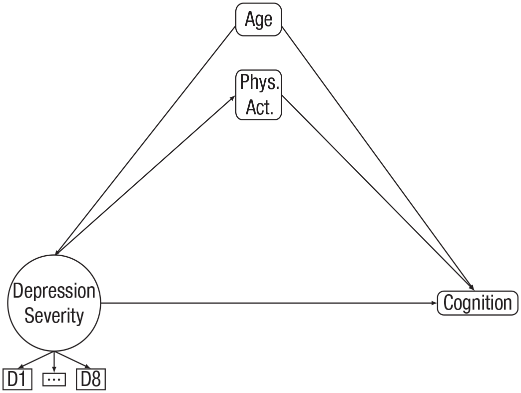
Model of depression severity, physical activity, and cognition, controlling for age.

In Figure 1, there is one circular node, three larger square nodes, and three smaller square nodes. The depression-severity construct is represented by the circular node, indicating it is a latent variable in this analysis. The three smaller square nodes below the depression-severity node represent the individual item indicators that comprise the latent variables for that construct (note that there are eight items, but we show “D1, . . . , D8” for simplicity of the model). The three larger square nodes are age, physical activity, and cognition, which were treated as manifest variables in this analysis. Note that some variables, such as physical activity here, can be manifest variables in some analyses and latent variables in other analyses, depending on the way in which they are measured and conceptualized. Other variables, such as depression severity, may be harder to directly measure and thus are often conceptualized as latent variables.

There are numerous pathways connecting the 12 nodes in Figure 1 (note that seven nodes, D2–D7, are summarized with the “ . . . ” node). Starting with the depression-severity node, there are pathways to each of the item indicators representing D1 through D8. These represent the loadings of individual items onto the latent factor, labeled “depression severity.” By convention, the arrows for loadings are directed from the latent factor to the individual measured items. This can be seen as an assumption that the underlying latent factor is a cause of the measured item score (Borsboom, 2005; Borsboom et al., 2003). There are also pathways from depression severity to physical activity and cognition representing hypothesized effects of depression severity on both physical activity and cognition. The estimates of these paths can be interpreted as if they were regression coefficients. Next, moving to the physical-activity node, there is a pathway to cognition (representing a hypothesized effect of physical activity on cognition). Finally, there are two pathways from age: one to depression severity and one to cognition. Age is included as a covariate in this model diagram to illustrate that we wanted to include the hypothesized effect of age on depression severity and cognition. Whereas in reality age likely plays a role in predicting physical activity (Godfrey et al., 2013), we left out this pathway in this didactic example.

The pathways of interest for our structural equation modeling analysis were those from depression severity to physical activity, from physical activity to cognition, from depression severity to cognition, from age to depression severity, and from age to cognition. For each of these five pathways, our SEM estimated a regression coefficient describing its strength and direction. Depression severity, age, physical activity, and cognition also have variances that were estimated in the analysis. We did not specify any covariances in this model diagram.

After specifying the model diagram in Figure 1, we fit the model to the data and compared the hypothesized (i.e., model-implied) variance–covariance matrix with the observed variance–covariance matrix.

In general, a researcher may wish to drop the indirect effects of depression severity to physical activity and physical activity to cognition by either not specifying these paths or fixing them to 0. This model would be considered nested because it would be a smaller version of the initial, or full, model. This “reduced” model would then be compared with the full model using a Δχ² test. A significant result (p < .05) would suggest the full model showed better fit than the reduced model, whereas a nonsignificant result would suggest the reduced model showed comparable fit with the full model. In the latter case, the reduced model would be preferred because it would be a more parsimonious representation of the data. Whereas the parsimony principle would suggest the “best” model is the simplest one, researchers should also consider the theory guiding their research question to determine whether a simpler model (i.e., direct or indirect) is more useful than a full (i.e., both direct and indirect) model. Nonnested models may also be compared by consulting the Akaike information criterion or Bayesian information criterion, in which smaller values suggest better fit (Kline, 2015; Vrieze, 2012). For more on structural equation modeling, nested-model comparison, and determining model fit, see Harlow (2014), Kline (2015), or Schumacker and Lomax (2016).

Following these steps, we fit and compared three models. Model 1 was considered the full model, with all five of the pathways estimated (depression severity to physical activity, physical activity to cognition, depression severity to cognition, age to depression severity, and age to cognition). Model 2 was considered the indirect-effects model, in which the pathway from depression severity to cognition was fixed to 0. Model 3 was considered the direct-effects model, in which the pathways from depression severity to physical activity and physical activity to cognition were fixed to 0. We established a priori that if the full model showed good fit to the data, it would be compared with the indirect and direct models. If significant differences were found using the Δχ² test, the full model would be retained for interpretation. If, however, no significant differences emerged, the more parsimonious model (indirect or direct) would be retained for interpretation. Each of these three models has different implications. The full model implies both direct and indirect (through physical activity) effects of depression on cognition are necessary to explain the relationship between depression and cognition. The direct model implies only the direct effect is necessary to explain this relationship. The indirect model implies only the indirect relationship is necessary.

We fit the full model and indirect- and direct-effects models to the synthetic data. All three models showed good fit to the data, except for the SRMR for the direct model and the χ² for each model. However, as discussed previously, a significant χ² alone is not enough to determine poor model fit. All fit indices results are reported in Table 1.

Table 1.

Structural Equation Modeling Fit Indices Results

Model	χ² (df)	CFI	RMSEA [90% CI]	SRMR	Δχ² (df)
Full	1225 (42)***	.98	.05 [.05, .05]	.06	—
Direct	2985 (44)***	.96	.08 [.07, .08]	.10	573 (2)***
Indirect	1472 (43)***	.98	.05 [.05, .06]	.07	88 (1)***

Note: CFI = comparative fit index; RMSEA = root mean square error of approximation; CI = confidence interval; SRMR = standardized root mean square residual. Δχ² refers to comparison with the full model.

***

p < .001.

The results of the Δχ² test showed a significant difference between the full and direct models and between the full and indirect models. This suggested that the additional pathways contained in the full model led to significant improvements over the direct or indirect models. Thus, the full model was retained as the final model for analysis (Harlow, 2014; Kline, 2015). The results of the full model are shown in Table 2 and Figure 2. They suggested a negative relationship between depression severity and physical activity (β = −0.26, p < .001), a negative relationship between depression severity and cognition (β = −0.07, p < .001), and a positive relationship between physical activity and cognition (β = 0.03, p < .001) after adjusting for age.

Table 2.

Full Model Results

Parameter	Unstandardized estimate (b)	Standard error	p value	Standardized estimate (β)
Depression severity to cognition	−0.31	0.03	< .001	−0.07
Physical activity to cognition	0.08	0.02	< .001	0.03
Age to cognition	0.24	0.002	< .001	0.75
Depression severity to physical activity	−0.35	0.02	< .001	−0.26
Depression severity to age	−0.01	0.001	< .001	−0.09

Fig. 2.

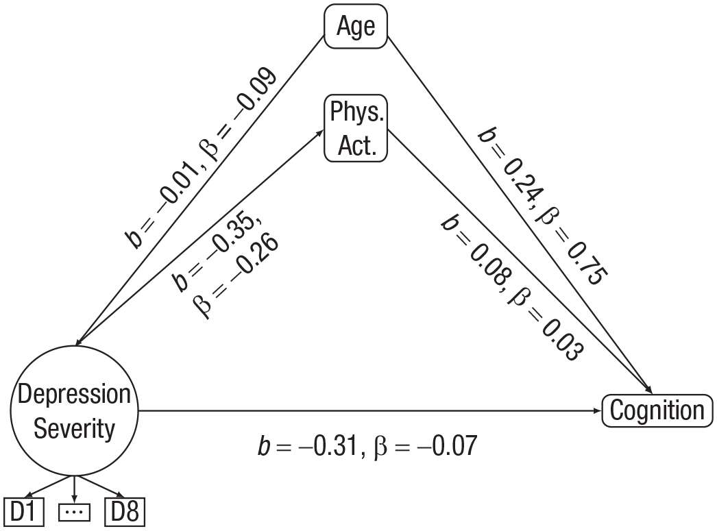
Structural equation modeling full-model results. β refers to the standardized estimates; b refers to the unstandardized estimates.

Causal DAG approach applied to the depression severity/cognition example

The results of the structural equation modeling analysis suggest that depression severity affects cognition indirectly through an effect on physical activity. However, depression and physical activity have a bidirectional association, meaning it is plausible physical activity preceded depression. A causal DAG approach can be useful in helping to think through the temporal ordering of variables and to make inferences about which variables actually caused which other variables. An example of such an approach follows. We present this approach as an alternative approach to the previous structural equation modeling analysis using the same synthetic data set.

We began by building the DAG shown in Figure 3. The exposure and outcome of interest should be added to the DAG first. Therefore, we began by adding depression severity and cognition. As stated previously, it is important to remember that in a DAG, the absence of an arrow is a stronger assumption than the presence of an arrow. Therefore, if we are interested in the effect of depression severity on cognition, we should start by ensuring that all common causes of depression and cognition are identified and added to the DAG. Existing literature suggests that common causes of depression/depressive symptoms and cognition include age, gender, education, and physical activity. These should be indicated on the DAG. Note that we refer here to physical activity as measured before depression assessment. This is crucial given both the time-varying nature of depression and physical activity and the bidirectional associations between them. Note that all arrows in the DAG represent moving forward in time.

Fig. 3.

Directed acyclic graph depicting the causal association between depression severity and cognition.

We must next consider whether any set of variables added to the DAG so far have common causes, add these to the DAG, and then continue this process in a recursive manner until all common causes are added. We must also consider how these common causes are linked with each other. We need not be limited by variables available in the data because the goal is to accurately depict the complete set of causal processes that gave rise to our data. Deciding when to stop adding common causes is a subjective decision. When satisfied that all common causes are on the DAG, the DAG can be used to identify which variables ought to be adjusted for in the statistical analysis.

For simplicity, we assume the DAG in Figure 3 comprehensively depicts all common causes among measured and unmeasured constructs (in reality, another researcher may choose to add additional common causes, such as genetic factors or other comorbid mental-health conditions). We can now use the DAG to determine which variables must be adjusted for. We can do this by identifying backdoor (i.e., biasing) paths from depression to cognition. In this case, backdoor paths include the following:

Depression severity ← Age → Cognition

Depression severity ← Gender → Cognition

Depression severity ← Education → Cognition

Depression severity ← Physical activity → Cognition

Depression severity ← Age → Physical activity → Cognition

Depression severity ← Age → Education → Cognition

Depression severity ← Gender → Education → Cognition.

To block all backdoor paths, age, gender, education, and physical activity (all measured before depression measurement) must be adjusted for. This is the sufficient set for adjusting for confounding. Note that no mediators or colliders are included in the sufficient set. After a sufficient set is established, researchers can choose from a variety of strategies for adjustment: Statistical control in a multivariable model, restriction, matching, and inverse probability weighting are some options. These decisions regarding adjustment can be applied to any model that best aligns with the type and distribution of the data (e.g., logistic regression, Cox regression, mixed models). For this example, we chose a multivariable linear regression model, adjusted for the sufficient set of confounders noted previously.

The results of the linear regression are shown in Table 3. In the unadjusted model, a 1-unit increase in CESD8 score (representing greater depression severity) was associated with lower cognition (β = −0.13, 95% confidence interval [CI] = [−0.12, −0.15]). After adjusting for the sufficient set of confounders identified with the DAG, this association persisted, although it was slightly attenuated (adjusted β = −0.06, 95% CI = [−0.04, −0.07]). This means that for every 1-unit increase in CESD8 score, the mean cognition score decreased by about 0.06 SD, adjusting for age, gender, education, and prior physical activity.

Table 3.

Results of DAG-Informed Analysis of the Association Between Depression Severity and Cognition Incidence

	Unadjusted model		Fully adjusted model^a
	Unstandardized estimate (b)	Standardized estimate (β)	Unstandardized estimate (b)	Standardized estimate (β)
1-unit increase in CESD8 score	−0.24 [−0.27, −0.21]	−0.13 [−0.12, −0.15]	−0.10 [−0.12, −0.08]	−0.06 [−0.04, −0.07]

Note: The 95% confidence intervals are shown in brackets. DAG = directed acyclic graph; CESD8 = Center for Epidemiological Studies–Depression Scale.

Adjusted for gender, age in years, years of education, and amount of moderate physical activity.

In interpreting our findings, note that in choosing variables for the sufficient set, we made the crucial assumption that the measures of physical activity reported in the 2016 sweep represented behavior before the day of the interview, that depression severity represented symptoms experienced on the day of the interview, and therefore that our measure physical activity represented behavior that preceded depression. Although we believed this was reasonable, if this assumption is not believed, one solution would be to use data on confounders measured in a previous study cycle, such as 2014 data. However, the use of earlier confounder data comes itself with an assumption—that the confounders measured in 2014 are sufficient to block backdoor paths observed on the DAG. This assumption may also be incorrect. If we were convinced that all backdoor paths had been sufficiently blocked by our analysis and that our assumptions about temporal ordering of the data were correct, then the adjusted result could be interpreted as a causal effect of increased depression severity on cognition.

This analysis did not consider mediation, but mediators could be added to the DAG to depict causal mechanisms—including physical activity—explaining the association between depression severity and cognition. The DAG in Figure 4 depicts mediation by physical activity following depression measurement. We can see from this DAG that although earlier measures of physical activity have an effect on depression, later values of physical activity are affected by depression and therefore are believed to lie on the causal pathway from depression severity to cognition. The DAG in Figure 4 demonstrates why we were careful not to adjust for physical activity measured after depression screening. Had we done so, we would have eliminated some of the causal effect we were attempting to measure. Note that if a researcher is specifically interested in mediation by physical activity following depression, then a separate causal-mediation analysis that includes these later constructs can be conducted (Richiardi et al., 2013; Valeri & VanderWeele, 2013). Such an analysis is beyond the scope of the current example.

Fig. 4.

Directed acyclic graph depicting the causal association between depression severity and cognition with time-varying health behaviors.

Discussion

Comparing SEMs and causal DAGs

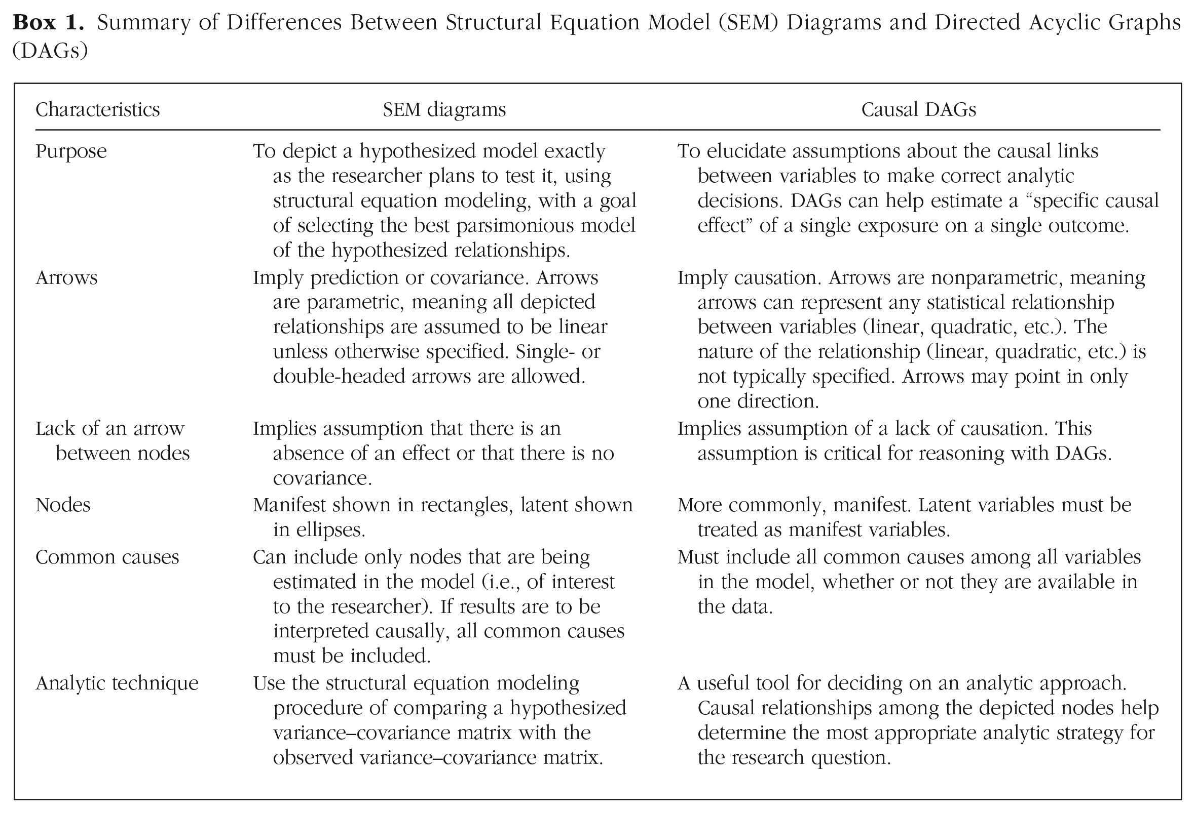
The similarities and differences between model diagrams for SEMs and causal DAGs are summarized in Box 1. The two key distinctions that should be highlighted are as follows.

Box 1.

Summary of Differences Between Structural Equation Model (SEM) Diagrams and Directed Acyclic Graphs (DAGs)

Characteristics	SEM diagrams	Causal DAGs
Purpose	To depict a hypothesized model exactly as the researcher plans to test it, using structural equation modeling, with a goal of selecting the best parsimonious model of the hypothesized relationships.	To elucidate assumptions about the causal links between variables to make correct analytic decisions. DAGs can help estimate a “specific causal effect” of a single exposure on a single outcome.
Arrows	Imply prediction or covariance. Arrows are parametric, meaning all depicted relationships are assumed to be linear unless otherwise specified. Single- or double-headed arrows are allowed.	Imply causation. Arrows are nonparametric, meaning arrows can represent any statistical relationship between variables (linear, quadratic, etc.). The nature of the relationship (linear, quadratic, etc.) is not typically specified. Arrows may point in only one direction.
Lack of an arrow between nodes	Implies assumption that there is an absence of an effect or that there is no covariance.	Implies assumption of a lack of causation. This assumption is critical for reasoning with DAGs.
Nodes	Manifest shown in rectangles, latent shown in ellipses.	More commonly, manifest. Latent variables must be treated as manifest variables.
Common causes	Can include only nodes that are being estimated in the model (i.e., of interest to the researcher). If results are to be interpreted causally, all common causes must be included.	Must include all common causes among all variables in the model, whether or not they are available in the data.
Analytic technique	Use the structural equation modeling procedure of comparing a hypothesized variance–covariance matrix with the observed variance–covariance matrix.	A useful tool for deciding on an analytic approach. Causal relationships among the depicted nodes help determine the most appropriate analytic strategy for the research question.

Key Distinction 1

SEM diagrams do not necessarily depict causal relationships, whereas causal DAGs are always meant to describe causal relationships. This affects the meaning and use of arrows. Because arrows in causal DAGs represent both causal relationships and the concept of temporality, it is crucial that each arrow points in a single direction. Because arrows in SEM diagrams do not necessarily imply causation, but rather covariance, double-headed arrows are allowed (Greenland & Brumback, 2002). Note that some users of both DAGs and SEMs include double-headed arrows as a shorthand for unknown common causes. Although this approach can simplify a complex graph, note that it technically violates the rules of a DAG (Haber et al., 2022).

Key Distinction 2

Structural equation modeling always uses the same general analytic technique (i.e., comparing a hypothesis with an observed covariance matrix), whereas causal DAGs are not associated with any particular statistical model. In structural equation modeling, the model diagram is drawn to reflect a specific model the researcher plans to test. In other words, a researcher simultaneously draws a model diagram and decides on an analytic strategy. DAGs, on the other hand, are best thought of as a tool that precedes statistical-analysis decisions. DAGs depict assumptions the researcher is comfortable making, and these assumptions can guide in choosing an analytic technique and aid in interpreting results.

Another important difference between a DAG-based analysis and a structural equation modeling analysis is that researchers typically do not consider model fit as a primary criterion for assessing a DAG-based analysis, and covariates in such an analysis should generally not be assessed for significance or removed to make the model more parsimonious because they are selected based on a priori knowledge.

Despite visual similarities, SEM diagrams and causal DAGs are used for different purposes, and choosing one is not necessarily an “either/or” question. There are considerations researchers should make when exploring the use of structural equation modeling or causal DAGs. If the research aim is to assess the relationships among multiple latent variables, structural equation modeling may be an appropriate tool. Indeed, structural equation modeling could be useful for researchers who wish to examine interrelationships among several mental-health constructs (e.g., depression and anxiety). Using different forms of structural equation modeling, psychiatric epidemiologists could study the direct and indirect effects of covariates on mental health (i.e., using path analysis or latent variable modeling) or study how change in one construct is related to change in another construct over time (i.e., using a form of longitudinal structural equation modeling called “parallel process modeling”; Newsom, 2015). Structural equation modeling is also useful when latent variables are involved in a research question because it can parse out measurement error on the individual items comprising the latent variable.

If the research question of interest is specifically a causal question, a causal DAG can be useful. Causal inference is becoming increasingly popular in psychological science because it allows causal claims to be made when a randomized controlled trial (RCT) cannot be conducted (Rohrer, 2018). Indeed, there are many situations in which an RCT cannot be conducted in psychological research. For example, researchers cannot randomly assign participants to develop symptoms of depression or anxiety, experience chronic stress, lose a loved one, or engage in substance use behavior. A researcher could use a causal DAG to depict the current state of knowledge regarding how variables are linked and then—if the researcher is willing to accept the assumptions outlined in the DAG—build a model that can elicit a causal effect of an exposure on an outcome of interest.

Can SEMs and DAGs be combined?

There may be situations in which a researcher wishes to combine the flexibility of structural equation modeling with the causal inference capabilities of DAGs. Such a combination is certainly possible because a DAG can be thought of as a “qualitative schematic” for a particular class of structural equation modeling (i.e., linear structural equation modeling), or a nonparametric SEM (VanderWeele & Rothman, 2021). Conversely, structural equation modeling may be thought of as an algebraic system for a causal DAG (VanderWeele & Rothman, 2021). Indeed, previous research suggesting SEMs cannot be causal has been criticized (Bollen & Pearl, 2013), and the field of structural causal models shows that researchers can readily combine principles of DAGs in a structural equation modeling framework (Pearl, 1998, 2012).

If a researcher does interpret the results of structural equation modeling causally, there are multiple strong assumptions that must be acknowledged. First, one must assume all confounding and collider stratification is correctly specified in the system of equations. The rules of causal DAGs described in this article can aid in ensuring this is the case. Second, one must assume that all relationships between variables are linear or otherwise specify the correct nature of the relationship among constructs. This is a very strong assumption, perhaps stronger than the graphical assumptions (VanderWeele & Rothman, 2021). In summary, structural equation modeling can be a powerful tool as long as certain strong assumptions hold. Even if these assumptions do not hold, it can be a useful hypothesis-generating tool (VanderWeele & Rothman, 2021). For more in this area, see Pearl (2012), Kline (2015, Chapter 8), and VanderWeele and Rothman (2021).

Conclusions and future directions

Researchers in the psychological sciences and psychiatric epidemiology often work together, so understanding the methodology and terminology used by each field is valuable—especially as psychology begins to adopt more causal-modeling concepts (Rohrer, 2018) and public health (especially psychiatric epidemiology) begins to adopt more latent-variable concepts (van de Pavert et al., 2017). Both SEM diagrams and DAGs are graphical tools for researchers to help conceptualize and guide their research. Structural equation modeling is a flexible analytical technique for modeling relationships among multiple constructs. DAGs are a tool for making decisions about which variables to adjust for so that associations can be interpreted causally. Psychologists and psychiatric epidemiologists can use these approaches in their work and may find it useful to become better acquainted with both approaches if they are familiar with only structural equation modeling or DAGs.

Footnotes

Transparency

Action Editor: Rogier A. Kievit

Editor: David A. Sbarra

Author Contribution(s)

Zachary J. Kunicki and Meghan L. Smith share first authorship.

Zachary J. Kunicki: Conceptualization; Formal analysis; Methodology; Writing – original draft.

Meghan L. Smith: Conceptualization; Formal analysis; Methodology; Writing – original draft.

Eleanor J. Murray: Conceptualization; Methodology; Project administration; Writing – review & editing.

ORCID iD

Zachary J. Kunicki

References

Altman

D. G.

Bland

J. M.

(1995). Statistics notes: Absence of evidence is not evidence of absence. BMJ, 311(7003), Article 485. https://doi.org/10.1136/bmj.311.7003.485

Bollen

K. A.

Pearl

(2013). Eight myths about causality and structural equation models. In Morgan

S. L.

(Ed.), Handbook of causal analysis for social research (pp. 301–328). Springer.

Borsboom

(2005). Measuring the mind: Conceptual issues in contemporary psychometrics. Cambridge University Press.

Borsboom

Mellenbergh

G. J.

van Heerden

(2003). The theoretical status of latent variables. Psychological Review, 110(2), 203–219. https://doi.org/10.1037/0033-295X.110.2.203

Brandt

Spencer

Folstein

(1988). The telephone interview for cognitive status. Neuropsychiatry, Neuropsychology, and Behavioral Neurology, 1(2), 111–117.

Butters

M. A.

Becker

J. T.

Nebes

R. D.

Zmuda

M. D.

Mulsant

B. H.

Pollock

B. G.

Reynolds

C. F.

(2000). Changes in cognitive functioning following treatment of late-life depression. American Journal of Psychiatry, 157(12), 1949–1954. https://doi.org/10.1176/appi.ajp.157.12.1949

Curran

P. J.

Cole

Bauer

D. J.

Hussong

A. M.

Gottfredson

(2016). Improving factor score estimation through the use of observed background characteristics. Structural Equation Modeling: A Multidisciplinary Journal, 23(6), 827–844. https://doi.org/10.1080/10705511.2016.1220839

Digitale

J. C.

Martin

J. N.

Glymour

M. M.

(2022). Tutorial on directed acyclic graphs. Journal of Clinical Epidemiology, 142, 264–267. https://doi.org/10.1016/j.jclinepi.2021.08.001

Folstein

M. F.

Robins

L. N.

Helzer

J. E.

(1983). The mini-mental state examination. Archives of General Psychiatry, 40(7), 812–812.

10.

Fried

E. I.

(2015). Problematic assumptions have slowed down depression research: Why symptoms, not syndromes are the way forward. Frontiers in Psychology, 6, Article 309. https://doi.org/10.3389/fpsyg.2015.00309

11.

Fried

E. I.

Nesse

R. M.

(2015). Depression sum-scores don’t add up: Why analyzing specific depression symptoms is essential. BMC Medicine, 13(1), Article 72. https://doi.org/10.1186/s12916-015-0325-4

12.

Fried

E. I.

Nesse

R. M.

Zivin

Guille

Sen

(2014). Depression is more than the sum score of its parts: Individual DSM symptoms have different risk factors. Psychological Medicine, 44(10), 2067–2076. https://doi.org/10.1017/S0033291713002900

13.

Ganguli

Dodge

H. H.

Ratcliff

G. G.

Chang

C.-C. H.

(2006). Depressive symptoms and cognitive decline in late life: A prospective epidemiological study. Archives of General Psychiatry, 63(2), 153–160. https://doi.org/10.1001/archpsyc.63.2.153

14.

Glymour

M. M.

Greenland

(2008). Causal diagrams. In Rothman

K. J.

Greenland

Lash

T. L.

(Eds.), Modern epidemiology (Vol. 3, pp. 183–209). Lippincott Williams & Wilkins.

15.

Godfrey

Lord

Galna

Mathers

J. C.

Burn

D. J.

Rochester

(2013). The association between retirement and age on physical activity in older adults. Age and Ageing, 43(3), 386–393. https://doi.org/10.1093/ageing/aft168

16.

Greenland

Brumback

(2002). An overview of relations among causal modelling methods. International Journal of Epidemiology, 31(5), 1030–1037. https://doi.org/10.1093/ije/31.5.1030

17.

Greenland

Pearl

Robins

J. M.

(1999). Causal diagrams for epidemiologic research. Epidemiology, 10(1), 37–48.

18.

Haber

N. A.

Wood

M. E.

Wieten

Breskin

(2022). DAG With Omitted Objects Displayed (DAGWOOD): A framework for revealing causal assumptions in DAGs. Annals of Epidemiology, 68, 64–71. https://doi.org/10.1016/j.annepidem.2022.01.001

19.

Harlow

L. L.

(2014). The essence of multivariate thinking: Basic themes and methods. Routledge.

20.

Hernán

M. A.

Robins

J. M.

(Eds.). (in press-a). Causal inference: What if. Chapman & Hall/CRC.

21.

Hernán

M. A.

Robins

(in press-b). Chapter 21: G-methods for time-varying treatments. In Hernán

M. A.

Robins

(Eds.), Causal inference: What if? Chapman & Hall/CRC.

22.

L.-t.

Bentler

P. M.

(1999). Cutoff criteria for fit indexes in covariance structure analysis: Conventional criteria versus new alternatives. Structural Equation Modeling: A Multidisciplinary Journal, 6(1), 1–55.

23.

Jansen

J. P.

Schmid

C. H.

Salanti

(2012). Directed acyclic graphs can help understand bias in indirect and mixed treatment comparisons. Journal of Clinical Epidemiology, 65(7), 798–807. https://doi.org/10.1016/j.jclinepi.2012.01.002

24.

Juster

F. T.

Suzman

(1995). An overview of the health and retirement study. The Journal of Human Resources, 30, S7–S56. https://doi.org/10.2307/146277

25.

Kline

R. B.

(2015). Principles and practice of structural equation modeling. The Guilford Press.

26.

Lei

P.-W.

(2007). Introduction to structural equation modeling: Issues and practical considerations. Educational Measurement: Issues and Practice, 26(3), 33–43. https://doi.org/10.1111/j.1745-3992.2007.00099.x

27.

Little

T. D.

Preacher

K. J.

Selig

J. P.

Card

N. A.

(2007). New developments in latent variable panel analyses of longitudinal data. International Journal of Behavioral Development, 31(4), 357–365. https://doi.org/10.1177/0165025407077757

28.

McArdle

J. J.

McDonald

R. P.

(1984). Some algebraic properties of the Reticular Action Model for moment structures. British Journal of Mathematical and Statistical Psychology, 37(2), 234–251. https://doi.org/10.1111/j.2044-8317.1984.tb00802.x

29.

McNeish

Wolf

M. G.

(2021). Dynamic fit index cutoffs for confirmatory factor analysis models. Psychological Methods. Advance online publication. https://doi.org/10.1037/met0000425

30.

Murray

E. J.

Kunicki

Z. J.

(2022). As the wheel turns: Causal inference for feedback loops and bidirectional effects. OSF Preprints. https://doi.org/10.31219/osf.io/9em5q

31.

Nebes

R. D.

Butters

M. A.

Mulsant

B. H.

Pollock

B. G.

Zmuda

M. D.

Houck

P. R.

Reynolds

C. F.

(2000). Decreased working memory and processing speed mediate cognitive impairment in geriatric depression. Psychological Medicine, 30(3), 679–691. https://doi.org/10.1017/S0033291799001968

32.

Newsom

J. T.

(2015). Longitudinal structural equation modeling: A comprehensive introduction. Routledge.

33.

Nowok

Raab

G. M.

Dibben

(2016). synthpop: Bespoke creation of synthetic data in R. Journal of Statistical Software, 74(11), 1–26. https://doi.org/10.18637/jss.v074.i11

34.

Paterniti

Verdier-Taillefer

M.-H.

Dufouil

Alpérovitch

(2002). Depressive symptoms and cognitive decline in elderly people: Longitudinal study. British Journal of Psychiatry, 181(5), 406–410. https://doi.org/10.1192/bjp.181.5.406

35.

Pearl

(1995). Causal diagrams for empirical research. Biometrika, 82(4), 669–688.

36.

Pearl

(1998). Graphs, causality, and structural equation models. Sociological Methods & Research, 27(2), 226–284.

37.

Pearl

(2000). Causality: Models, reasoning, and inference. Cambridge University Press.

38.

Pearl

(2012). The causal foundations of structural equation modeling. In Hoyle

R. H.

(Ed.), Handbook of structural equation modeling (pp. 68–91). The Guilford Press.

39.

Quintana

D. S.

(2020). A synthetic dataset primer for the biobehavioural sciences to promote reproducibility and hypothesis generation. eLife, 9, Article e53275. https://doi.org/10.7554/eLife.53275

40.

Rhemtulla

van Bork

Borsboom

(2020). Worse than measurement error: Consequences of inappropriate latent variable measurement models. Psychological Methods, 25(1), 30–45. https://doi.org/10.1037/met0000220

41.

Richardson

T. S.

Evans

R. J.

Robins

J. M.

Shpitser

(2017). Nested Markov properties for acyclic directed mixed graphs. arXiv https://doi.org/10.48550/arXiv.1701.06686

42.

Richiardi

Bellocco

Zugna

(2013). Mediation analysis in epidemiology: Methods, interpretation and bias. International Journal of Epidemiology, 42(5), 1511–1519. https://doi.org/10.1093/ije/dyt127

43.

Robins

(1986). A new approach to causal inference in mortality studies with a sustained exposure period—Application to control of the healthy worker survivor effect. Mathematical Modelling, 7(9), 1393–1512. https://doi.org/10.1016/0270-0255(86)90088-6

44.

Robins

J. M.

Hernán

M. Á.

Brumback

(2000). Marginal structural models and causal inference in epidemiology. Epidemiology, 11(5), 550–560. https://doi.org/10.1097/00001648-200009000-00011

45.

Rohrer

J. M.

(2018). Thinking clearly about correlations and causation: Graphical causal models for observational data. Advances in Methods and Practices in Psychological Science, 1(1), 27–42. https://doi.org/10.1177/2515245917745629

46.

Savalei

(2014). Understanding robust corrections in structural equation modeling. Structural Equation Modeling: A Multidisciplinary Journal, 21(1), 149–160. https://doi.org/10.1080/10705511.2013.824793

47.

Schumacker

Lomax

(2016). A beginner’s guide to structural equation modeling (4th ed.). Routledge.

48.

Shrier

Platt

R. W.

(2008). Reducing bias through directed acyclic graphs. BMC Medical Research Methodology, 8(1), Article 70. https://doi.org/10.1186/1471-2288-8-70

49.

Suzuki

Shinozaki

Yamamoto

(2020). Causal diagrams: Pitfalls and tips. Journal of Epidemiology, 30(4), 153–162. https://doi.org/10.2188/jea.JE20190192

50.

Turvey

C. L.

Wallace

R. B.

Herzog

(1999). A revised CES-D measure of depressive symptoms and a DSM-based measure of major depressive episodes in the elderly. International Psychogeriatrics, 11(2), 139–148. https://doi.org/10.1017/S1041610299005694

51.

Valeri

VanderWeele

T. J.

(2013). Mediation analysis allowing for exposure–mediator interactions and causal interpretation: Theoretical assumptions and implementation with SAS and SPSS macros. Psychological Methods, 18(2), 137–150.

52.

van de Pavert

Sunderland

Luijten

Slade

Teesson

(2017). The general relationship between internalizing psychopathology and chronic physical health conditions: A population-based study. Social Psychiatry and Psychiatric Epidemiology, 52(10), 1257–1265.

53.

VanderWeele

T. J.

(2012). Invited commentary: Structural equation models and epidemiologic analysis. American Journal of Epidemiology, 176(7), 608–612. https://doi.org/10.1093/aje/kws213

54.

VanderWeele

T. J.

Lash

T. L.

Rothman

K. J.

(2021). Analysis of interaction. In Lash

T. L.

VanderWeele

T. J.

Haneuse

Rothman

K. J.

(Eds.), Modern epidemiology (4th ed., pp. 619–653). Wolters Kluwer.

55.

VanderWeele

T. J.

Rothman

K. J.

(2021). Formal causal models. In Lash

T. L.

VanderWeele

T. J.

Haneuse

Rothman

K. J.

(Eds.), Modern epidemiology (4th ed., pp. 33–51). Wolters Kluwer.

56.

Vrieze

S. I.

(2012). Model selection and psychological theory: A discussion of the differences between the Akaike information criterion (AIC) and the Bayesian information criterion (BIC). Psychological Methods, 17(2), 228–243. https://doi.org/10.1037/a0027127

A Primer on Structural Equation Model Diagrams and Directed Acyclic Graphs: When and How to Use Each in Psychological and Epidemiological Research

Abstract

Keywords

What Is Structural Equation Modeling?

Elements of a SEM diagram

Nodes

Arrows/paths

Analytic technique

Mediators

Latent variables

What Is a DAG?

Elements of a DAG

Nodes

Arrows/paths

Fundamental structures in DAGs

Mediators

Confounders

Colliders

Interaction

Analytic technique

Novel applications of DAGs

Applied Example: Applying Structural Equation Modeling and DAG Concepts to the Study of the Association Between Depression Severity and Cognition

SEM applied to the depression severity/cognition example

Causal DAG approach applied to the depression severity/cognition example

Discussion

Comparing SEMs and causal DAGs

Key Distinction 1

Key Distinction 2

Can SEMs and DAGs be combined?

Conclusions and future directions

Footnotes

Transparency

ORCID iD

References