
Abstract
The cross-lagged panel model (CLPM) is a widely used technique for examining reciprocal causal effects using longitudinal data. Critics of the CLPM have noted that by failing to account for certain person-level associations, estimates of these causal effects can be biased. Because of this, models that incorporate stable-trait components (e.g., the random-intercept CLPM) have become popular alternatives. Debates about the merits of the CLPM have continued, however, with some researchers arguing that the CLPM is more appropriate than modern alternatives for examining common psychological questions. In this article, I discuss the ways that these defenses of the CLPM fail to acknowledge well-known limitations of the model. I propose some possible sources of confusion regarding these models and provide alternative ways of thinking about the problems with the CLPM. I then show in simulated data that with realistic assumptions, the CLPM is very likely to find spurious cross-lagged effects when they do not exist and can sometimes underestimate these effects when they do exist.
The cross-lagged panel model (CLPM) is a widely used technique for examining causal processes using longitudinal data (Duncan, 1969; Finkel, 1995; Heise, 1970). With at least two waves of data, it is possible to estimate the association between a predictor at Time 1 and an outcome at Time 2 after controlling for a measure of the outcome at Time 1. With some assumptions, this association can be interpreted as a causal effect of the predictor on the outcome. The simplicity of the model along with its limited data requirements have made the CLPM a popular choice for the analysis of longitudinal data. For instance, Usami, Murayama, and Hamaker (2019) reviewed medical-journal articles published between 2009 and 2019 and found 270 articles that used this methodological approach. A broader search of Google Scholar returned more than 4,500 articles that used the term “cross-lagged panel model” in the last 40 years. 1
The CLPM expands on simpler cross-sectional analyses by controlling for contemporaneous associations between the predictor and outcome when predicting future scores on the outcome. Presumably, confounding factors should be reflected in this initial association, which would mean that any additional cross-lagged associations between the Time 1 predictor and the Time 2 outcome would reflect a causal effect of the former on the latter (again, with some assumptions). Hamaker et al. (2015) pointed out, however, that the CLPM does not adequately account for stable-trait-level associations, and they proposed the random-intercept CLPM (RI-CLPM) as an alternative (also see Allison, 2009; Berry & Willoughby, 2017; Zyphur et al., 2020). The RI-CLPM includes stable-trait-variance components that reflect variance in the predictor and outcome that is stable across waves. Hamaker et al. showed that failure to account for these random intercepts and the associations between them can lead to incorrect conclusions about cross-lagged effects. This critique of the CLPM has already been cited frequently and has had an important impact on researchers who use longitudinal data (Lüdtke & Robitzsch, 2021; Usami, 2021).
Despite this impact, debates about the relative merits of the CLPM versus the RI-CLPM (and other alternatives) continue. Most notably, Orth et al. (2021) argued that sometimes researchers are actually interested in the associations that a classic CLPM tests and that the choice of model should depend on one’s theories about the underlying process. Orth et al.’s article has already been cited almost 200 times even though it was published only approximately 1 year ago at the time of this writing. Many of the citing articles justified their use of the CLPM on the basis of the arguments that Orth et al. put forth. Asendorpf (2021) presented similar arguments to those raised by Orth et al. and warned that alternatives to the CLPM, such as the RI-CLPM, should not be used to model long-term longitudinal data, a warning echoed by Lüdtke and Robitzsch (2021).
The goal of the current article is to examine these defenses of the CLPM. I focus first on the interpretation of models like the RI-CLPM that include a stable-trait component, followed by simulations that demonstrate the problems with the CLPM and the utility of its alternatives. These simulations show that when the standard lag-1 CLPM is used, cross-lagged effects are often biased, and the likelihood of finding significant spurious effects can reach 100% in many realistic scenarios. At the same time, the CLPM can underestimate cross-lagged effects when they do exist. Because in most areas of psychological research sources of stability beyond those that are modeled in the standard lag-1 CLPM are likely to exist, the CLPM will usually be misspecified and should not be used for causal inference from longitudinal data.
Between-Persons and Within-Persons Associations: Implications for Model Choice
In their critique of the CLPM, Hamaker et al. (2015) described the RI-CLPM as a multilevel model that separates between-persons associations from within-persons associations. But what is a between-persons association, and how does it differ from a within-persons association? Why is it important to separate these levels of analysis when examining lagged causal effects? These questions are critical because answers to them form the basis for some debates—and misunderstandings—about the CLPM.
For instance, Orth et al. (2021) relied heavily on the description of the cross-lagged paths in the RI-CLPM as within-persons effects in their defense of the CLPM. They stated that “a potential disadvantage of the proposed alternatives to the CLPM is that they estimate within-person prospective effects only, but not between-person prospective effects” (p. 1014) and that “in many fields researchers are also interested in gaining information about the consequences of between-person differences” (p. 1014). They went on to argue that “a limitation of the RI-CLPM is that it does not provide any information about the consequences of between-person differences. In the RI-CLPM, the between-person differences are relegated to the random intercept factors” (p. 1026). They then stated that “the RI-CLPM includes [an] unrealistic assumption, specifically that the between-person variance is perfectly stable” (p. 1026). Orth et al. did acknowledge later in their article that “some portion of the systematic between-person variance will be included in the residualized factors” (p. 1026). However, they argued that this discrepancy is a conceptual problem for the RI-CLPM: They stated that “the cross-lagged effects in the RI-CLPM are not pure within-person effects but partially confounded with between-person variance” (p. 1026). These statements—statements that form the basis of Orth et al.’s defense of the CLPM—do not accurately describe the RI-CLPM and its relation to the CLPM.
In this section, I explain why the between-person effects that Orth et al. (2022) and Asendorpf (2021) hope to obtain are unlikely to be accurately estimated using the CLPM. I then argue that their claims about the limitations of the RI-CLPM and related models are incorrect. These models do, of course, have limitations, so I also briefly discuss additional models beyond the RI-CLPM that can address at least some of the conceptual concerns about the RI-CLPM that remain after these misconceptions are corrected.
A note about models and terminology
At this point, it is necessary to introduce more formally the models discussed in this article and to clarify the terminology that I use when describing the components of the models. As Falkenström et al. (2022) noted, “it is important to first reflect on the relevance of [a statistical analysis method] to the real-world processes a researcher attempts to model” and that “researchers familiar with the study subject can make educated guesses about the nature of this process” (p. 447). It has long been recognized that psychological variables often have features that are both “state-like” and “trait-like” (Hertzog & Nesselroade, 1987). In other words, these variables exhibit stability and change, and it is possible to think about different ways that constructs can stay the same or change over time.
For instance, Nesselroade (1991) noted that there are at least three types of latent factors that are frequently very useful for explaining variability in repeated measures of individual difference constructs—state factors, slowly changing factors that reflect an autoregressive process, and completely stable-trait factors (also see Kenny & Zautra, 2001). State factors are the most fleeting because they reflect variance that is unique to a single measurement occasion. These state factors can include random measurement error, but they can also include any reliable variance that does not carry over from one wave to the next. If a construct consisted solely of state variance, there would be no stability over time. In contrast, stable-trait factors reflect variance that is perfectly stable across all waves of assessment. If a construct consisted solely of stable-trait variance, then wave-to-wave stability would be perfect regardless of the length of the interval between them. In between these two extremes are slowly changing trait factors in which variance at one wave predicts variance at the next, but with less than perfect stability. Kenny and Zautra (2001) labeled this as “autoregressive trait” variance to reflect the fact that there is some trait-like stability (reflected in a nonzero stability coefficient from one wave to the next) and change over the long term. Stability of this autoregressive trait factor declines with increasing interval length. Of course, these three components do not exhaust all possible patterns of stability and change (see e.g., Usami, Murayama, & Hamaker, 2019; Zyphur et al., 2020), but they reflect reasonable assumptions about features that are likely to generalize to a wide range of psychological variables.
It is possible to frame the CLPM and its modern alternatives in the context of these sources of variance. Figure 1a shows a diagram of the model that has been the focus of this article: the CLPM. 2 Although the CLPM can be drawn using only observed variables, Figure 1 includes latent variables to emphasize the relation to its more complex alternatives. In a CLPM with two variables X and Y, the model includes one latent variable per wave for each. These latent variables have an autoregressive structure (hence, the “AR” label in the figure) such that people’s current standing is a function of their past standing, linked through a stability parameter. Note that the CLPM does not include any measurement error for the indicators. This means that the latent variables from the autoregressive part of the model are equivalent to the observed variables (which is why it is also possible to draw an equivalent CLPM with only observed variables). The CLPM assumes that all variance is of the slowly changing, autoregressive variety described by Nesselroade (1991). The cross-lagged associations from X at Time T – 1 to Y at Time T (or more precisely, the lagged associations between the respective AR variables) are meant to capture the causal effects of X on Y.

Diagram of the three models used in this article. (a) The cross-lagged panel model (CLPM). (b) The random-intercept CLPM (RI-CLPM). (c) The stable trait, autoregressive trait, state (STARTS) model.
Figure 1b shows the diagram of the RI-CLPM. The difference between the CLPM and the RI-CLPM is that the RI-CLPM includes a random intercept that accounts for “time-invariant, trait-like stability” (Hamaker et al., 2015, p. 104). The random intercept corresponds to purely stable trait variance and is thus labeled “Stable Trait” in the figure. Including this stable-trait component changes the meaning of the autoregressive part of the model. Whereas in the CLPM the cross-lagged paths reflect associations between the X and Y variables over time, in the RI-CLPM, these paths reflect associations among wave-specific deviations from a person’s stable-trait level. This is what allows for the separation of between- and within-persons associations and the interpretation of the cross-lagged associations as causal effects (Hamaker et al., 2015; Usami, 2021).
Note that the CLPM is nested within the RI-CLPM; the CLPM is equivalent to the RI-CLPM with the random-intercept (or stable-trait) variance constrained to 0. This also means that if one tries to fit the RI-CLPM to data with no stable-trait variance, the RI-CLPM reduces to the CLPM and the interpretation of the within-persons or autoregressive part of the model will be identical to the interpretation of the CLPM. This will be a critical point when evaluating the validity of Orth et al.’s (2021) critiques of the RI-CLPM and related models.
The final model, presented in Figure 1c, is the bivariate stable trait, autoregressive trait, state (STARTS) model (Kenny & Zautra, 1995, 2001), which I have not yet mentioned but will play a role in the later simulations. The STARTS model differs from the RI-CLPM in that it includes a wave-specific state component (labeled “S” in the figure), which reflects variance in an observed variable that is perfectly state-like and unique to that occasion. This state component can include measurement error or any reliable variance that is unique to a single wave of assessment. The idea that some amount of pure state variance would exist in measures of psychological constructs is quite plausible (Fraley & Roberts, 2005), but simpler models such as the RI-CLPM have often been preferred because the STARTS requires more waves of data than the RI-CLPM and often has estimation problems (e.g., Cole et al., 2005; Orth et al., 2021; Usami, Todo, & Murayama, 2019).
Recently, Usami, Murayama, and Hamaker (2019) clarified that the CLPM, RI-CLPM, STARTS model, and many other longitudinal models could be thought of as variations of an overarching “unified” model that captures many different forms of change (Usami, 2021). Because debates about the utility of the CLPM have primarily focused on debates about the inclusion of the random intercept, I focus in this article primarily on the comparison of the CLPM to the RI-CLPM and the STARTS model because this comparison highlights these debates most clearly. It is certainly true, however, that if the other forms of change included in the unified model were part of the actual data-generating process, then all the models covered in this article would be misspecified and could lead to biased estimates.
As a final terminological note, when describing results from the models, I try to reserve the term “effects” for paths that can be interpreted as causal links from one variable to another, and I use the term “associations” for empirical links in which causality is not assumed or cannot be determined. I occasionally (and necessarily) deviate from this usage when describing certain claims about what these models can and cannot do (e.g., when describing certain between-persons effects). I describe effects as “spurious” when they are intended to reflect causal effects but do not. 3
Does the CLPM provide estimates of between-persons causal effects?
Orth et al. (2021) noted that one reason to prefer the CLPM over alternatives such as the RI-CLPM is that the lagged associations in the CLPM capture between-persons causal effects, whereas in the alternatives, they do not. Can the cross-lagged paths in the CLPM be interpreted in this way? Unfortunately, in most cases, they cannot, at least with the standard CLPM. This is because a critical assumption underlying the CLPM is likely to be violated in the types of data that psychologists and many other social scientists typically use. Specifically, an important assumption in the CLPM is that the wave-specific disturbances (the us in Fig. 1a) are uncorrelated with each other and with variables measured at prior waves (Heise, 1970). Any unmeasured variable that results in (unmodeled) correlations between these wave-specific disturbances will invalidate the interpretation of the cross-lagged associations as causal effects. Examples of factors that would invalidate these causal interpretations include unmeasured stable-trait components, unmeasured time-invariant predictors, or unmeasured time-varying predictors with some degree of stability.
It is possible to evaluate the plausibility of this assumption by examining patterns of stability over time in real data and then comparing these patterns with the patterns of stability that would be implied by models like the CLPM. Figure 2 provides an example of such a comparison. To begin, consider a single variable that has a lag-1 autoregressive structure such that current standing on that variable is determined by past standing (through a stability parameter) and a disturbance term. Figure 2a shows the implied stability coefficients over various intervals for three hypothetical variables, each with a lag-1 autoregressive structure. The three lines represent variables that differ in their 1-year stability, which range from .75 (shown in the top line) to .25 (shown in the bottom line). For variables with a lag-1 autoregressive structure, the stability over any number of intervals is a function of the stability across one interval raised to the power of the number of intervals that have elapsed. So the expected correlation for a measure with a 1-year stability of .75 assessed over a 2-year period would be .752 = .56. The expected correlation over a 3-year period would be .753 = .42. Figure 2a shows that for variables with a lag-1 autoregressive structure, stability coefficients are expected to decline quickly as intervals lengthen, even for variables that were initially quite stable. If actual stability coefficients observed in real data decline more slowly than what is shown in Figure 2a, then this would suggest that the variable under consideration does not have a lag-1 autoregressive structure.
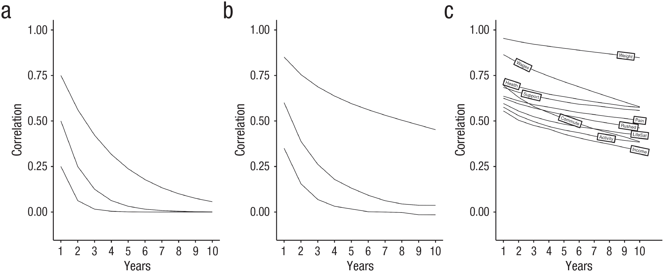
Implied and actual stability over increasing time lags. (a) Data generated from a lag-1 autoregressive model with no cross-lagged paths. (b) Data generated from a model with cross-lagged effects. (c) Data show the actual stability of 10 diverse variables from a panel study.
The standard CLPM builds on this simple lag-1 autoregressive model, extending it to include lagged, reciprocal associations between two or more variables. If there are positive lagged effects from a positively correlated predictor that itself has some stability, then stability coefficients for the outcome will decline more slowly than if the variable had a simple lag-1 autoregressive structure. Figure 2b shows the implied stability coefficients for data generated from a model that is consistent with a true cross-lagged process. Comparing Figure 2b with Figure 2a shows the existence of these cross-lagged associations slows the decline in stability coefficients. These differences are most pronounced in variables with high initial stabilities. Note that in this example, I set all cross-lagged effects to be .20, an effect that is in the 90th percentile of cross-lagged effects found in a recent meta-analysis of articles that used the CLPM (Orth et al., 2022). This choice will likely underestimate the typical decline in stabilities that emerge with increasing interval length in real data. 4 But how do these compare with patterns of stability that are found in real data?
As a comparison, I used real longitudinal data to examine the typical pattern of stability coefficients for a wide range of variables. Specifically, I selected 10 diverse variables 5 that have been included in almost every wave of the long-running Household Income and Labour Dynamics in Australia (HILDA) panel study, which now spans 20 waves of assessment (Watson & Wooden, 2012). I intentionally selected variables from different domains, variables that might have different psychometric properties because of how easily observable they are (e.g., weight and income are likely to be measured with less systematic and random error than life satisfaction or social support), and variables that might change in different ways over time. Stability coefficients across lags ranging from 1 to 10 years are shown in Figure 2c.
A comparison of Figure 2b and Figure 2c shows that stability coefficients for this diverse set of real-world variables decline more slowly (usually considerably more slowly) than would be predicted by a lag-1 autoregressive model or a lag-1 CLPM model with substantial cross-lagged effects. These patterns of stability coefficients suggest that additional sources of stability contribute to these patterns, and stability in these unmeasured variables would invalidate the causal conclusions one would normally draw from the CLPM (Heise, 1970). Thus, the standard CLPM is unlikely to accomplish the goal of estimating between-persons causal effects that Orth et al. (2021) articulated. 6 Models like the RI-CLPM were designed to address precisely this problem.
Between-persons and within-persons associations: ambiguous terminology
In the previous section, I argued that even if one accepts Orth et al.’s (2021) characterization of the differences between the CLPM and its modern alternatives, the CLPM will usually not be able to support the types of between-persons causal conclusions that they say they want to draw. However, it is also important to carefully examine the claims that Orth et al. (and others, e.g., Asendorpf, 2021) made about these models because doing so reveals problems with their interpretation of the differences that exist between these models. Indeed, Orth et al.’s primary complaints about the RI-CLPM are based on incorrect interpretations of the alternatives to the CLPM.
Orth et al. (2021) criticized the RI-CLPM for assuming that all between-persons differences are perfectly stable over time and for removing all between-persons variance from the within-persons associations (see p. 1026), but those descriptions are not correct. In the RI-CLPM and other related models, between-persons variance is simply “defined” as the variance that is “perfectly” stable over time. This is an issue of terminology, not assumptions.
To illustrate, I again refer to Figure 1a and Figure 1b, which show the relationship between the CLPM and RI-CLPM. According to the terminology of Hamaker et al. (2015), the within-persons part of the model is the part that specifies the associations among the AR variables over time. Remember, however, that the CLPM is nested within the RI-CLPM. This means that if one fits the RI-CLPM to data for which there is no stable-trait variance, the RI-CLPM simply reduces to the CLPM. What one is left with in this case is the within-persons part of the model, which is now perfectly equivalent to the CLPM. Thus, what Orth et al. (2021) referred to as a between-persons model (the CLPM) is actually the within-persons part of the RI-CLPM, and what Orth et al. referred to as a between-persons effect would be considered a within-persons effect in the RI-CPLM. Indeed, relying on the terminology of the RI-CLPM, the CLPM would be said to assume that no between-persons variance exists whatsoever. Again, the terminology is the problem.
This confusion about precisely how the RI-CLPM separates within- and between-persons associations and effects likely results from ambiguity in the terms used to describe them. Certain aspects of the between/within distinction are clear and unambiguous. When data are collected from multiple participants at a single point in time, there can only be between-persons variance. All associations that can be observed in these data are necessarily between-persons associations. For instance, in cross-sectional data, a negative correlation between self-esteem and depression can be interpreted only as a between-persons association: People who score high on measures of self-esteem tend to score low on measures of depression. If, on the other hand, just a single individual is assessed repeatedly over time, all variance is within-persons variance, and all associations would be within-persons associations. For example, if a single person’s self-esteem and depression were tracked over time, a negative correlation would reflect a within-persons association: When self-esteem is high in that individual, feelings of depression tend to be low.
The potential for confusion about these labels arises, however, when data are collected from multiple people across multiple occasions. Such data include information both about how people differ from one another (between-persons variance) and how each person changes over time (within-persons variance). Describing associations unambiguously as “between” versus “within” becomes more challenging with these multilevel data. The decision to label an association as “between” or “within” is not always linked in a straightforward way to the type of data that contribute to the effect. 7 The RI-CLPM does separate between-persons associations from within-persons associations, but it does not do so by “[relegating] between-person differences . . . to the random intercept factors” (Orth et al., 2021, p. 1026). Just as the CLPM links between-persons variance in a predictor to between-persons variance in an outcome measured at a later time, the within-persons part of the RI-CLPM does so, too.
This is important because the descriptions provided by Orth et al. (2021), Asendorpf (2021), and others suggest that the interpretation of the within-persons effects from the RI-CLPM is fundamentally different than the interpretation of the cross-lagged paths in the CLPM. For instance, Lüdtke and Robitzsch (2021) warned that the RI-CLPM would be “less appropriate [than the CLPM] for understanding the potential effects of causes that explain differences between persons” because the within-persons effects that it estimates are based on scores that “only capture temporary fluctuations around individual person means” (p. 18). Although it is true that the RI-CLPM cannot be used to investigate causal effects of stable individual differences, neither can the CLPM: The CLPM does not model the effects of those individual person means. In fact, the CLPM assumes that no individual differences in person means exist because the only person means from which the within-persons parts are deviated in the RI-CLPM are those for the perfectly stable trait. If that assumption is correct, then the interpretation of the CLPM will be identical to the RI-CLPM because the latter reduces to the former; if the assumption is wrong, then the CLPM is misspecified, and the lagged paths are not interpretable as causal effects for the reasons discussed in the prior section. The within-persons components of models like the RI-CLPM are no more “temporary” or “fluctuating” than are the components of the CLPM because the CLPM starts with the assumption that no stable-trait variance exists. The goal of the RI-CLPM is usually not to answer a fundamentally different question than what has traditionally been addressed using the CLPM; it is to address similar questions while controlling for the biasing effects of stable-trait variance.
Alternatives to the RI-CLPM
At this point, I note that there are alternatives to the models discussed so far that may come closer than the CLPM to capturing what critics of the RI-CLPM claim to want to assess. In discussing their support for the CLPM, neither Orth et al. (2021) nor Asendorpf (2021) denied that purely stable-trait variance exists in the data they typically examine even though its existence would invalidate the use of the simple lag-1 CLPM for causal inference (Heise, 1970). They objected, however, to separating purely stable between-persons variance from between-persons variance that changes slowly over time in an autoregressive manner when estimating cross-lagged effects.
For instance, Asendorpf (2021) stated (in the context of a substantive example of parental overvaluation affecting the childhood narcissism) that “it is the chronicity of overvaluation that makes children narcissistic, and this chronicity is captured only if the full range of between-person differences in chronic overvaluation is taken into account” (p. 831). Presumably Asendorpf is interested in a process by which a stable predictor (e.g., parental overvaluation) affects the amount or likelihood of change in an outcome from each wave to the next. Models like the RI-CLPM and STARTS model would not be able to capture the causal effect of the stable trait on changes at each wave. There are, however, alternatives that attempt do so while still accounting for the between-persons associations that models like the RI-CLPM are meant to address (see e.g., Dishop & DeShon, 2022; Gische et al., 2021; Lüdtke & Robitzsch, 2022; Murayama & Gfrörer, 2022; Usami, 2021; Zyphur et al., 2020).
Figure 3 illustrates one version of a dynamic panel model (for an accessible introduction, see Dishop & DeShon, 2022; for a comparison of dynamic panel models to alternatives like the RI-CLPM, see Lüdtke & Robitzsch, 2022; Murayama & Gfrörer, 2022). These models are designed to capture dynamic processes over time while accounting for unobserved heterogeneity (i.e., the unmeasured stable individual difference factors that bias estimates in simpler models). A critical difference between the RI-CLPM and this dynamic panel model is the precise way that the lagged effects are modeled. In the RI-CLPM, the lagged effects are attached to the within-persons components of the model, which reflect deviations from the stable trait (see Fig. 1b). In contrast, in the dynamic panel model and its variants, the lagged effects are attached directly to the observed variables, as shown in Figure 3. Notice that paths from the time-invariant latent factor 8 flow through the observed predictor to the observed outcome. In this model, for instance, the path from X2 to Y3 incorporates any association between the time-invariant factor associated with X and change in Y from Wave 2 to 3.

Diagram of the dynamic panel model.
By modeling these associations this way, the model incorporates an “accumulating” factor (Usami, 2021). This term reflects the fact that influence of the time-invariant factor accumulates over time: It affects observations at each wave directly and indirectly through all prior waves. The inclusion of an accumulating factor means that the dynamic panel model is not a multilevel model that cleanly separates between- and within-persons levels (Murayama & Gfrörer, 2022). Like the RI-CLPM, however, the model can still account for person-level factors that might bias the cross-lagged associations (Dishop & DeShon, 2022). So even if Orth et al. (2021) objected to the removal of perfectly stable trait associations from the lagged effects in the multilevel RI-CLPM, the dynamic panel model would not be subject to this criticism. A detailed discussion of the dynamic panel model and its relation to the RI-CLPM is beyond the scope of this article, but a number of recent articles have compared these models in detail, and readers are referred to them for further discussion (e.g., Lüdtke & Robitzsch, 2022; Murayama & Gfrörer, 2022).
Beyond Between and Within
In the previous sections, I discussed ambiguity in the labeling of between- and within-persons associations, focusing on how these ambiguities might lead to misinterpretations of models that include a stable-trait component. Considering alternatives to the multilevel framing of critiques of the CLPM—for instance, by focusing more precisely on principles of causal inference—might help clarify why the CLPM leads to incorrect conclusions and how models like the RI-CLPM or the dynamic panel model can help solve this problem (Rohrer & Murayama, 2021). However, even the causal-inference framing may be unfamiliar to researchers who rely on the CLPM. Therefore, it can be useful to highlight the problems of the CLPM in even simpler terms.
Specifically, it is easy to show that the simple correlations between stable-trait factors can masquerade as cross-lagged effects when the CLPM is used. As a demonstration, I generated two waves of data for two variables, X and Y. Figure 4a shows the data-generating process, which is a very simple correlated-latent-trait model. I set the variance of X and Y to be 1 and the reliability of the indicators to be .5. X and Y are associated only at the stable-trait level (r = .7). In other words, X and Y are related only because people who tend to score high on X on average also tend to score high on Y on average; X does not cause changes in Y or vice versa, and they have no unique associations across waves that cannot be accounted for by the stable-trait association. Figure 4b shows what happens if the CLPM is fit to the generated data. As shown, there would be clear evidence for reciprocal associations between the two even though there are no over-time causal effects of X on Y. The CLPM cannot distinguish between associations that occur at the stable-trait level from those that involve causal effects of one variable on another. 9

Spurious cross-lagged effects in data with only between-persons associations. (a) The data-generating model. (b) Estimates from the cross-lagged panel model (CLPM) fit to the generated data. Coefficients are unstandardized estimates. Residuals are not shown but are included.
Thus, Figure 4 provides an alternative way of thinking about the problems with the CLPM and the benefits of alternative models that incorporate something like a stable-trait component. Models like the RI-CLPM are useful because they test a very plausible alternative explanation of the underlying pattern of correlations that is being modeled when the CLPM is used, an alternative explanation that has nothing to do with causal effects of the predictor on the outcome. When stable-trait variance exists, cross-lagged paths in the CLPM can result entirely from associations at the stable-trait level, entirely from causal effects from one variable to the other, from some combination of the two, or from the effects of other unmeasured variables.
The logic of the CLPM is very similar to the logic of any other regression model in which researchers assess whether one variable predicts another after controlling for relevant confounds. When researchers test whether Time 1 X predicts Time 2 Y after controlling for Time 1 Y, they hope to capture whether there is something unique about X—something that cannot be explained by the concurrent association between X and Y—that helps them predict Y at a later time. But as Westfall and Yarkoni (2016) pointed out when discussing the difficulty of establishing incremental predictive validity of any kind, if the measure that they include as a control (i.e., Time 1 Y) is not a perfect measure of what researchers are trying to account for, then it is possible—indeed, quite easy—to find spurious incremental validity effects. Referring to Figure 4, Y1 is an imperfect measure of the latent variable Y. Thus, controlling for Y1 does not control for all of the association between X and Y, which means that X1 will still have incremental predictive validity of Y2 even after controlling for Y1.
Orth et al. (2021) acknowledged that they do indeed believe that the CLPM estimates causal effects. They stated that in the context of their focal case study of self-esteem and depression, “the hypothesized causal effect” in the CLPM can be stated to be that “when individuals have low self-esteem (relative to others), they will experience a subsequent rank-order increase in depression compared to individuals with high self-esteem” (p. 1014). Although this description of the cross-lagged path is technically correct, Orth et al. did not explain how this association can be interpreted as a causal effect. Unfortunately, when stable-trait variance exists in the measures being analyzed, then the estimated cross-lagged paths in a standard lag-1 CLPM will not reflect causal effects. Referring again to Figure 4b, it is technically correct to say that a substantial path from X1 to Y2 would show that individuals who score high on X1 have a rank-order increase in Y from Wave 1 to Wave 2, but this would be due solely to the effect of the stable trait reflected in the latent Y variable. The rank-order on Y changes from Time 1 to Time 2 not because of any causal effect of X but because the rank-order at Y1 imperfectly reflects the true rank-order of Y, and X is related to this rank ordering.
In summary, psychological constructs will very often have patterns of stability that are consistent with the existence of some form of stable, person-level influences. When such influences exist, a critical assumption of the lag-1 CLPM will be violated. In such cases, the lagged associations in a standard CLPM cannot be interpreted as causal effects. Considering the multilevel structure of the data and applying appropriate multilevel models (as reflected in the RI-CLPM; Hamaker et al., 2015) is one way to address this issue. Alternatively, models that account for these unmeasured person-level factors through other means can address this issue in different ways (e.g., in dynamic panel models; Dishop & DeShon, 2022).
When defending the CLPM, Orth et al. (2021) and Asendorpf (2021) did not take either approach. Instead, they simply asserted that the effects from the CLPM are meaningful even in the presence of stable-trait variance. Orth et al. claimed to want to test a “between-person prospective effect” but did not define what a between-persons prospective effect is, and they offered no causal analysis that explains the meaning of such an effect. Asendorpf went so far as to assert that using models that include a stable-trait component leads to cross-lagged “effects [that] are severely underestimated” (p. 830). Note, however, that he did not provide any evidence supporting that claim, including either simulation-based evidence from a known data-generating process or mathematical analyses of what these models estimate. It is easy to show, however, that when the CLPM is used, it is possible to mistake purely between-persons associations for over-time associations. I now turn to a set of simulations that demonstrate just how bad this problem likely is.
It Is Extremely Easy to Find Spurious Cross-Lagged Effects
The issues discussed in the previous sections show that hypothetically, it is possible to mistake stable-trait-level associations for causal effects when the CLPM is used. But how likely are such spurious effects? Unfortunately, it is extremely easy to find spurious cross-lagged effects under conditions that are quite likely in the typical situations in which the CLPM is used. Hamaker et al. (2015) and Usami, Todo, and Murayama (2019) conducted simulations to show that the estimates from a cross-lagged panel model were often biased in realistic situations. I do not think they went far enough, however, in describing the practical implications of these simulations or showing just how likely spurious effects are in realistic situations. So in the rest of this article, I build on their simulations and try to clarify when such spurious effects are likely to occur. As I show, there are many realistic scenarios in which researchers are almost guaranteed to find spurious cross-lagged effects.
The simulations
When considering what types of situations to simulate, I focused on realistic scenarios for the types of data to which the CLPM is likely to be applied (Fraley & Roberts, 2005). For instance, it is likely that most variables that psychologists (and other social and health scientists) choose to study over time have a longitudinal structure in which stability declines with increasing interval length (reflecting an autoregressive structure), yet this decline approaches or reaches an asymptote at which further increases in interval length are no longer associated with declines in stability (reflecting the influence of a stable trait). It is also likely that most measures of psychological constructs have some amount of pure state variance, which could reflect measurement error or true state-like influences.
To provide some context for these simulations, I again used real data from the 10 variables from the HILDA panel study that I used for the illustration in Figure 2. I then fit the most inclusive of the three models discussed earlier (the STARTS model) to see how much variance each component (stable trait, autoregressive trait, and state) accounted for. The proportion of variance for each of the three components and the stability coefficient for the autoregressive component are shown in Table 1.
Variance Components and Stability Estimates From the STARTS Model for 10 Variables in the HILDA

Note: The first three columns reflect the proportion of total variance accounted for by that component. The fourth column is the estimated stability of the autoregressive component. All variables were assessed in each of the 20 waves except commuting, which was included in all but Wave 1, and weight, which was included in the 15 most recent waves. STARTS = stable trait, autoregressive trait, state; HILDA = Household Income and Labour Dynamics in Australia.
The first thing to note from Table 1 is that there are substantial stable-trait components for all 10 variables. 10 Second, although the size of stable-trait variance component varies across the 10 variables, it is often comparable in size and sometimes exceeds the estimates for the autoregressive component that is the focus of the CLPM. Finally, for almost all the variables that were analyzed, the state component is also quite large, often accounting for one quarter to one third of the variance in these measures. These estimates can be used to evaluate the plausibility of the values that I chose for the simulation studies.
I used the simulations to test how variation in these factors affects the estimated cross-lagged paths when the CLPM is used. A Shiny app is available in which variations of this data-generating model can be specified and the effects on cross-lagged paths can be tested: http://shinyapps.org/apps/clpm/. 11 Readers can use this app to examine the specifications described in the text and to test alternatives.
Because the focus of this article is on examining the effects of unmodeled stable-trait variance, I set the variance of the stable-trait component for the predictor and outcome to be 1 in the primary simulations (although occasionally, I do set stable-trait variance to 0 to address specific questions). I then varied the ratio of autoregressive variance to stable-trait variance across four levels: 0, 0.5, 1, and 2. Likewise, I varied the ratio of nonstate to total variance across three levels: .5, .7, and .9. 12 The results in Table 1 show that these values correspond to what one might find in real data. Finally, I varied the size of the correlation between the stable traits across four levels from weak to very strong: .1, .3, .5, and .7. I ran 1,000 simulations for each of five sample sizes: 50, 100, 250, 500, and 1,000. In all simulations, I set the correlation between the initial autoregressive variance components for the predictor and outcome to be .50 and the stability parameter linking subsequent waves of the autoregressive components to be .50 (although later, I discuss some modifications to this). I also set the correlations between state components to be 0. Most importantly, all true cross-lagged paths were set to be 0. Consistent with the canonical STARTS model, I included a stationarity constraint so that variances, correlations, and stability coefficients are constrained to be equal over time. This constraint is not absolutely necessary, but it simplifies discussion of the estimated cross-lagged paths because there is just one estimate per model.
After generating the data, I tested a simple two-wave CLPM, keeping track of the average size of the estimated cross-lagged path coefficients and the number of cross-lagged coefficients that were significant at a level of .05. Note that researchers are often interested in determining which of the two variables in the model has a causal impact on the other rather than on simply testing the effect of one predictor on an outcome. Thus, an effect of X on Y, Y on X, or both would often be interpreted as a “hit” in common applications of the CLPM. This means that error rates are typically elevated in the CLPM even without unmodeled stable-trait associations unless corrections for multiple comparisons are used. In these simulations, I report the percentage of runs that result in at least one significant cross-lagged effect (out of two tested), and these can be compared with a baseline error rate of approximately 10%, assuming multiple comparisons are ignored.
Finally, although I focus on the common two-wave CLPM design, note that more waves of data lead to increased power to detect smaller effects—even spurious effects. This means that spurious cross-lagged effects are more likely to be found with better, multiwave designs. Thus, I also present results from simulations with more waves of data after presenting the primary results. Code used to generate the data, test the models, and run the simulation are available at https://osf.io/4qukz/. All analyses were run using R (Version 4.2.2; R Core Team, 2021). 13
Simulation results
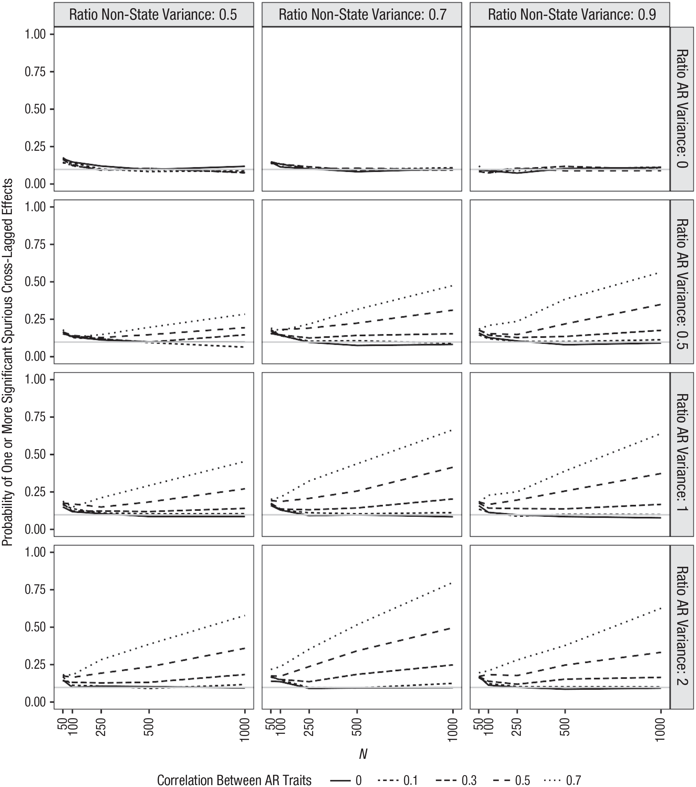
The proportion of simulations that resulted in at least one significant (spurious) cross-lagged effect in this initial simulation are presented in Figure 5. The y-axis reflects the percentage of runs in which a significant cross-lagged effect was found. Each x-axis shows results for different sample sizes. The columns reflect variation in the ratio of nonstate to total variance of the measures (which is equivalent to the reliability of the measure if state variance consists only of random error). The rows reflect variation in the ratio of autoregressive variance to stable-trait variance. The individual lines in each plot reflect different correlations between the two stable traits. The averaged estimates for the cross-lagged effects in each set of simulations (averaging across sample sizes because this will not affect the estimated effect) are reported in Table 2. What do these simulations tell researchers about when spurious effects are likely?

Simulation results for two-wave cross-lagged panel model. Columns reflect different ratios of nonstate to total variance. Rows reflect different ratios of autoregressive to stable-trait variance. Lines reflect different correlations between stable-trait components. Gray line reflects expected number of significant effects that are due to chance (assuming a critical p of .05).
Average Estimated Cross-Lagged Paths in Each Simulation Condition

Note: AR ratio = ratio of autoregressive variance to stable-trait variance.
When constructs have some stable-trait structure
If the measures include some amount of stable-trait variance—even if the stable traits are uncorrelated—it is likely that spurious cross-lagged effects will emerge. To be clear, this is most problematic when there is considerable stable-trait variance, when these stable traits are correlated, and when the correlation is quite high. However, error rates are elevated across most simulations. For instance, consider results in the third column of Figure 5, where most of the variance is nonstate variance. Specifically, focus on the fourth row, where there is relatively little stable-trait variance. This panel reflects the least problematic set of values tested, and even here, error rates approach 100% when correlations between the stable traits are strong (r = .70) and sample sizes are moderately large (N = 1,000). Even when correlations are more moderate (e.g., r = .5), however, these error rates approach 50% in large samples.
Error rates are not always monotonically associated with the size of the correlation between the stable traits. Consider the panels in Rows 2, 3, and 4 of Column 3. In these panels, where state variance is low and the ratio of autoregressive variance to stable-trait variance is .5 or higher, the error rates for the lowest correlation tested (r = .1, shown in the solid line) are actually higher than error rates for a higher stable-trait correlation of .3. A look at the actual estimates across simulations in Table 2 provides insight into why this is. The second through fourth rows of the fourth column in Table 2 show that the average estimated cross-lagged effects are negative when state variance is low, the correlation between the stable traits is low, and there is a substantial amount of autoregressive variance. These negative estimates emerge even though all associations among the latent components were specified to be positive.
This can be demonstrated even more clearly by simulating data with uncorrelated stable traits, an equal amount of autoregressive and stable-trait variance, and no state variance whatsoever (this simulation is not shown). In this case, the estimated cross-lagged paths will be approximately –.07. This is because by failing to account for the stable trait, the model overestimates the stability of X and Y, which means that the observed correlation between X at Time 1 and Y at Time 2 is lower than what would be expected based on the initial correlation between X and Y at Time 1 and the stability over time. 14 These simulations show that when the variables being examined have a trait-like structure, this can lead to spurious cross-lagged effects even when the stable-trait variance is not correlated. When correlations at the stable-trait level are strong, however, the effects of ignoring the stable-trait structure can be substantial. In some realistic scenarios (e.g., moderate correlations between stable traits, 70% of variance accounted for by nonstate components, and sample sizes over 100), significant spurious cross-lagged paths are almost guaranteed.
Note that the size of the spurious effects (which can also be thought of as the extent of bias in these estimates) shown in Table 2 are consistent with the size of estimated cross-lagged effects typically found in the literature. For instance, Orth et al. (2022) sampled from articles that used the CLPM to determine how large these effects typically are. In their analysis, the 25th, 50th, and 75th percentiles for cross-lagged effects were .03, .07, and .12. Even the largest of these values is similar to the spurious effects found in realistic scenarios from the simulations. 15
When measures have error or reliable occasion-specific variance
The simulations described above focus on situations in which the ratio of nonstate to total variance is very high, or in other words, when state variance is low. When there is a lot of state variance, including either reliable state variance or even just measurement error, this effect gets worse—potentially much worse. Consider the panel in the first row and the first column of Figure 5. In this case, the ratio of nonstate to total variance is set to .5, and there is no autoregressive variance. Note that values in this range are not unrealistic because this ratio is reduced both by the existence of measurement error and reliable occasion-specific variance. In this scenario, error rates are very high, approaching 100% with large samples even when the stable-trait correlation is just .3. Samples of 100 can result in spurious cross-lagged effects approximately 60% of the time when stable traits are correlated .5. Even in samples as small as 50, error rates exceed 25% in many situations.
This outcome is actually quite easy to understand. Indeed, we do not really need simulations at all to predict it. This result is a simple consequence of the issues that Westfall and Yarkoni (2016) discussed and those that I highlighted in Figure 4. Because the latent X and Y traits are measured imperfectly on each occasion, controlling for Time 1 Y when predicting Time 2 Y from Time 1 X does not fully account for the true association between X and Y. There will still be a residual association between Time 1 X and Time 2 Y, which can be accounted for by the freed cross-lagged path in the CLPM. The RI-CLPM (and the STARTS model) are useful because they do a better job accounting for this underlying association than the CLPM.
At this point, I highlight the fact that at least some of these effects are due more to the existence of measurement error (or reliable state variance) than to the existence of the stable trait. For instance, it is possible to simulate data with an autoregressive structure, to set the variance of the stable trait components to be 0, and to specify no cross-lagged paths. Even with a relatively high ratio of nonstate to total variance (e.g., .8 for this simulation, which is not shown), the average estimated cross-lagged paths would be .05, and spurious effects would be found 37% of the time in a two-wave design with samples of 500 participants. Again, Westfall and Yarkoni’s (2016) explanation can account for these results: The existence of measurement error or state variance in the observed measures of Y means that controlling for Y1 does not control for enough. The result is a spurious cross-lagged effect.
I also note that measurement error and reliable state variance also affect estimates from the RI-CLPM. If we specify a data-generating process that includes all three sources of variance (stable trait, autoregressive trait, and state/measurement error) but no cross-lagged paths, the CLPM will find substantial cross-lagged effects, but so will the RI-CLPM (at least if the autoregressive components of X and Y are correlated). To demonstrate, I simulated data with the following characteristics. The X and Y stable traits had variances of 1 and a correlation of .5, and X and Y autoregressive traits had a variance of 1 and a starting correlation of .5 with stability coefficients of .5. As before, I specified there to be no true cross-lagged effects, yet the average estimated cross-lagged effect from the RI-CLPM was .07. This would be easily detectable with moderate to large sample sizes and is similar in size to the typical cross-lagged effect found in the literature (Orth et al., 2022).
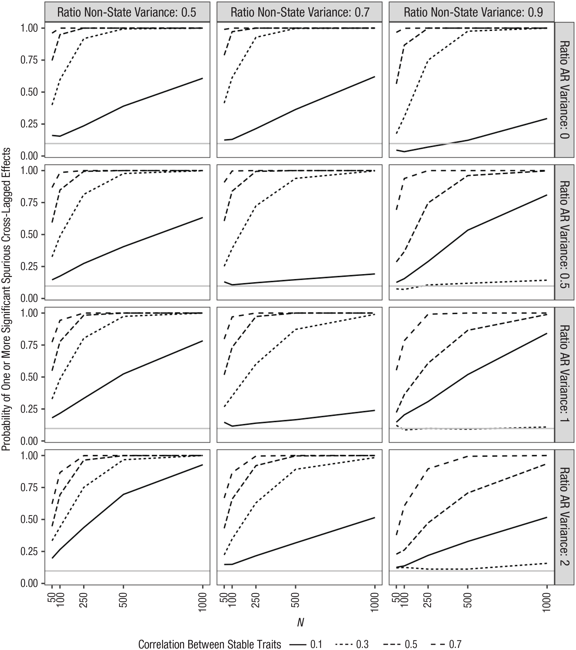
To examine this issue more systematically and to compare the likelihood of finding spurious effects when using the RI-CLPM with the likelihood when using the CLPM, I repeated the primary simulation using the RI-CLPM. Because the estimates of the cross-lagged paths are not affected by the size of the correlation between the stable-trait components when the RI-CLPM is used, instead of varying the correlation between stable traits, I varied the correlation between the initial wave autoregressive components. In addition, the RI-CLPM requires three waves of data instead of the two that I used in the initial simulation. The results are shown in Figure 6.
Simulation results for three-wave random-intercept cross-lagged panel model (RI-CLPM). Columns reflect different ratios of nonstate to total variance. Rows reflect different ratios of autoregressive to stable-trait variance. Lines reflect different correlations between autoregressive-trait components. Gray line reflects expected number of significant effects that are due to chance (assuming a critical p of .05).
As shown in Figure 6, when there is measurement error variance or reliable state variance, then there is a chance for spurious cross-lagged effects even when the RI-CLPM is used. To be sure, these effects are much less likely than with the CLPM: Error rates typically exceeded only 25% with large samples and very strong correlations between the autoregressive traits, whereas they often approached 100% with the CLPM. Note that this limitation of the RI-CLPM is not an argument for the CLPM (although it is an argument for using the STARTS model or other more complicated models when possible).
One response to the above simulations is to suggest that researchers simply need to use very reliable measures or perhaps model latent variables at each occasion instead of relying on observed variables with less than perfect reliability. This will certainly help, but it is important to remember that the “state” component in the STARTS model includes measurement error and reliable occasion-specific variance. Reliable state variance will affect these results in exactly the same way as random measurement error. Unfortunately, researchers do not know how common this reliable state component is in real data, although there is at least some evidence that it can exist and be large enough to be meaningful (Anusic et al., 2012; Lucas & Donnellan, 2012). Thus, even the use of latent occasions in the CLPM cannot solve this problem.
When there are many assessment waves
Although the CLPM is often used with just two waves of assessment, it can also be used with more complex data. Indeed, a general rule for longitudinal data is that more waves are better than fewer, and in situations in which stationarity could reasonably be expected, including more waves and imposing equality constraints should lead to more precise estimates of cross-lagged paths. When estimating true effects, this has the benefit of increasing power. When spurious effects would be expected, however, the use of more waves will also increase the probability of those spurious effects being significant (again, for a discussion of how factors that improve power can increase the ability to find spurious effects, see Westfall & Yarkoni, 2016).
Figure 7 shows a set of simulations that are similar to those reported in Figure 5, but this time using five waves of data and the CLPM with equality constraints across waves. When comparing these two figures, the effect of increasing the number of waves is immediately apparent: Error rates increase considerably. For instance, in the very realistic scenario of a sample size of 250, a correlation between stable traits of .5, nonstate variance ratio of .7, and a 1:1 ratio of stable-trait to autoregressive variance, the error rate increases from 58% to 97% when moving from a two-wave study to a five-wave study. With five waves of data, error rates often exceed 50%, even in samples as small as 50. So features that are generally desirable—large sample sizes and multiple waves of assessment—increase the likelihood of finding spurious cross-lagged effects. 16
Simulation results for five-wave cross-lagged panel model (CLPM). Columns reflect different reliabilities. Rows reflect different ratios of autoregressive to stable-trait variance. Lines reflect different correlations between stable-trait components. Gray line reflects expected number of significant effects that are due to chance (assuming a critical p of .05).
Modeling stable traits is not conservative
The examples above focused on cases in which there were no true cross-lagged effects in the data-generating model. The simulations showed that spurious effects are often very likely to be found. This pattern matches the intuition that models such as the RI-CLPM and STARTS model (which include a stable-trait component) are more conservative than the CLPM (Asendorpf, 2021). However, failure to model associations between stable-trait components can also lead to the underestimation of real cross-lagged effects. For instance, consider a situation in which the measures are perfectly reliable (and there is no reliable state variance) and the stable trait and autoregressive trait contribute equally (in this particular case, I also specified the correlations among the stable trait and autoregressive traits to be .5). If we simulate data with cross-lagged paths of .5 from X to Y and .2 from Y to X, the RI-CLPM reproduces these effects perfectly. However, even with no measurement error, the estimates from the CLPM are half the size that they should be, approximately .25 and .10.
The precise way that estimates will be affected depends on the size of these variance components and the correlations between them. Table 3 shows the results from a separate simulation that examines these effects. Specifically, because the parameter estimates were the focus (rather than the frequency of errors), I followed Lüdtke and Robitzsch (2021) and generated just one set of 10,000 responses for each of 48 combinations. I varied the correlation between the stable traits across four levels: .1, .3, .5, and .7. Likewise, I varied the correlation between the autoregressive traits across the same four levels. I also varied the ratio of autoregressive to trait variance across three levels: 0.5, 1, and 2. For this example, state variance was set to be 0, and the stability of the autoregressive components was set to .5. Table 3 shows only results for one cross-lagged path, for which the true value is .50.
Estimated Cross-Lagged Path in Each Simulation Condition When True Value = .5

Note: AR r = correlation between autoregressive components; AR ratio = ratio of autoregressive variance to stable-trait variance. State variance is set to 0 for all simulations.
First, consider the example just discussed. Looking at the column where the correlation between the stable traits is .5 and the row where the correlation between the autoregressive traits is .5 and the ratio of autoregressive variance to stable-trait variance is 1, the true cross-lagged effect of .5 is estimated to be .25. One can then move up and down that column or across that row to see the effects of the other factors on this underestimation. For instance, looking at the values in the rows immediately above and below this value shows that the underestimation of the cross-lagged effects is greater when there is more stable-trait variance than when there is less. The true cross-lagged effect of .50 is estimated to be .17 when there is twice as much stable-trait variance as autoregressive variance, whereas it is estimated to be .33 (still an underestimate, but not as bad) when there is twice as much autoregressive variance as stable-trait variance.
Moving across the same row shows how this estimate is affected by variation in the correlation between stable traits. As shown, the estimate for a true cross-lagged effect of .50 declines from .31 when the correlation between the stable traits is a high .70, to .25 when the correlation is .50, to .2 when the correlation is .30, and to .18 when the correlation is .1. Again, stable-trait variance affects estimates of cross-lagged effects even when the stable traits are weakly correlated or uncorrelated.
Finally, moving across groups of rows (e.g., Rows 1–3 compared with Rows 4–6) shows the effect of the correlation between autoregressive components. In this case, the estimate of the cross-lagged parameter is negatively associated with the size of the correlation between autoregressive components, declining from .32 when the correlation between autoregressive components is .10 to .19 when the correlation is .70 (again, for the example in which the stable-trait correlation is .5 and there is an equal amount of autoregressive and stable-trait variance).
These simulations show that including a stable-trait component is not more conservative than excluding it when testing cross-lagged effects. Indeed, when true cross-lagged effects exist, the CLPM can often underestimate them when there is stable-trait variance. Again, this pattern is predictable just by considering tracing rules for structural equation models. When stable-trait variance exists, the stability of the observed variables is overestimated in a CLPM, resulting in a corresponding underestimation of the cross-lagged paths in most situations. If researchers observe a pattern in which cross-lagged effects routinely emerge when the CLPM is used but disappear when a stable trait is modeled, then this would suggest that the effects themselves are likely spurious.
When considering the implications of this finding, there are two things to keep in mind. First, although the CLPM can underestimate the true cross-lagged effects, this may not result in decreased power to detect these effects relative to alternative models such as the RI-CLPM. This is partly because models that separate between-persons associations from within frequently have less bias, but at the cost of efficiency; the standard errors in such models are often greater than models that do not correctly separate levels (for an explanation, see Allison, 2009; for similar examples, see Usami, Todo, & Murayama, 2019). Second, it is difficult to consider how to think about power in the context of the CLPM, where it is so easy to find spurious effects. Indeed, I ran simulations similar to those described earlier but with true cross-lagged effects. However, when simulating data in which one cross-lagged path was zero and the other was greater than zero, estimated “power” to detect both the true effect and the spurious one was quite high.
The second thing to remember is that the above simulations were conducted specifying that the measures are perfectly reliable and that there is no occasion-specific state variance. This is unlikely in practice. Indeed, when state variance is included, the estimates from the RI-CLPM are also biased. The precise way that state variance affects estimates is a quite complicated function of all the factors included in the previous simulations, the state factor, and the sign of the correlations and true cross-lagged paths. Because of this complexity, these simulations are beyond the scope of this article, although the Shiny app is provided for readers to examine the effect of different combinations on estimated cross-lagged paths. Note that the STARTS model is appropriate for modeling data that include stable-trait, autoregressive-trait, and state variance. Although the STARTS model has been somewhat underused in the literature because of frequent estimation problems, recent methodological advances in Bayesian modeling have helped address these concerns (Lüdtke et al., 2018).
Moving Forward With (or Without) the CLPM
After describing the various approaches available to model longitudinal data, Orth et al. (2021) made the following recommendation: “Before selecting a model, researchers should carefully consider the psychological or developmental process they would like to examine in their research, and then select a model that best estimates that process” (p. 1018). There are two problems, however, when using this guidance to advocate for the CLPM. First, the CLPM is explicitly and inarguably a model of constructs that change over time. The model is misspecified when used to describe variables that have a stable-trait structure or other sources of stability that are omitted from the model. Of course, it is a truism to say that “all models are wrong,” but it is rare to select a model that is known to be wrong in such a fundamental way, especially when more appropriate models exist. The mathematics of the model and the simulations provided in this and other articles show that this clear misspecification can frequently lead to spurious effects in realistic scenarios. So if researchers’ careful consideration of the psychological and developmental processes under examination leaves open the possibility that the variables have some stable-trait structure, then the CLPM will be the wrong choice.
Even if we ignore the misspecification involved when applying the CLPM to data with a stable-trait structure, there is an additional problem with Orth et al.’s (2021) guidance. If there is a plausible alternative model that describes the data as well as (or better than) the preferred model, then additional work is needed to defend that preferred model. The CLPM cannot rule out the plausible alternative explanation that cross-lagged paths are due to simple between-persons correlations, and thus, researchers would need to justify their belief that this source of variance does not exist in the data they are modeling before the results of the CLPM would be interpretable.
Note that although Asendorpf (2021) unequivocally asserted that cross-lagged effects are “severely underestimated” when models that include a stable trait are used, he provided no evidence to support this claim (p. 830). Neither he nor Orth et al. (2021) proposed a data-generating process that can be shown to lead to correct results when modeled using the CLPM but that would result in biased estimates or incorrect conclusions if modeled using more modern alternatives. Generating data from the model that these authors said should often be preferred—the CLPM—results in correct estimates (despite the possibility of inadmissible solutions because of negative estimated variances) when analyzed using the RI-CLPM or STARTS model. Note that Lüdtke and Robitzsch (2021) did identify data-generating processes that lead to biased estimates when the resulting data are analyzed using the RI-CLPM, but their results do not show that the CLPM is more appropriate than the RI-CLPM in these situations. 17
In addition to the conceptual reasons for abandoning the CLPM that I discussed in this article, the simulations show that relying on the CLPM when the variables in the model have some stable-trait variance leads to dramatically inflated error rates (often reaching 100% in realistic scenarios, even with small to moderate sample sizes). The constructs that psychologists study very rarely have a purely autoregressive structure. At some point, the long-term stabilities of most constructs are stronger than would be suggested by the short-term stabilities and the length of time that has elapsed alone. This is likely due to the fact that many constructs have at least some stable-trait variance that is maintained over time (even if that stable-trait variance reflects something such as response styles or other method factors). And if there is stable-trait variance, it is quite plausible that two constructs correlate at the stable-trait level. Models such as the RI-CLPM and STARTS model provide a way to test this compelling and plausible model and to adjust for the problematic effects of these stable-trait components when testing reciprocal effects.
So if using the CLPM results in dramatically elevated error rates for cross-lagged effects when they do not exist while having the potential to underestimate these effects when they do exist (again, sometimes dramatically in realistic scenarios), should researchers ever rely on the CLPM for causal analyses? Given these concerns, it would seem prudent to abandon the use of the CLPM for causal analysis of longitudinal data. When at least three waves of data are available, models like the RI-CLPM can be used. If no stable-trait variance exists, these models will simply reduce to a CLPM.
To be sure, there are certain situations when alternatives to the CLPM cannot be used, most notably in the very common situation in which only two waves of assessment are available. This creates an important challenge for the field given that most studies that use the CLPM have only two waves of data available (Hamaker et al., 2015; Usami, Todo, & Murayama, 2019). However, as Figure 4 showed, there are too many plausible alternative models that can lead to the same set of six correlations among two variables at two time points to draw any conclusions about which of those models is correct. Many have suggested that two-wave designs barely count as “longitudinal” (e.g., Ployhart & MacKenzie, 2014; Rogosa, 1995), and the reasons for this claim are quite salient when considering the application of the CLPM to such data. There is simply not enough information available in these data to distinguish among multiple competing models.
In discussing reciprocal associations using cross-lagged analyses, Rogosa (1995) noted that there is a
hierarchy of research questions about longitudinal data [that] might start with describing how a single attribute—say aggression—changes over time. A next step would be questions about individual differences in change of aggression over time, especially correlates of change in aggression. Only after such questions are well understood does it seem reasonable to address a question about feedback or reciprocal effects. (p. 34)
Many researchers have noted that this first step—describing how a construct changes over time—is not possible with only two waves of data (e.g., Fraley & Roberts, 2005; Ployhart & MacKenzie, 2014; Rogosa, 1995).
Given the ubiquity of two-wave designs in psychological and medical research (Usami, Todo, & Murayama, 2019), an inevitable question is “What should we do with studies that have only two waves of data?” Longitudinal data are often difficult and expensive to collect, and researchers understandably want to get the most out of the data that they have spent so much time (and often money) to collect. Personally, given the issues discussed in this article, I believe that the CLPM is almost always the wrong choice even when it is the only choice. However, I recognize that not everyone will agree, and therefore, it is worthwhile to consider what else can be done to minimize the problems of the CLPM. One step in this direction would be for researchers who use the CLPM with two-wave studies to explicitly discuss the plausibility of the assumptions that underlie it (e.g., that no stable-trait variance or other omitted sources of stability exist in the measures that have been assessed).
For instance, with two waves of data, it is impossible to distinguish between a simple correlated-latent-trait model and a model with no stable trait and cross-lagged effects (i.e., the competing models shown in Fig. 4). One way that researchers could approach this dilemma would be to fit and show results for both models and then describe any theory or prior empirical evidence that supports the acceptance of one model over the other. This would require researchers to be explicit that something beyond the data themselves is required to evaluate the plausibility of their chosen model. As Grosz et al. (2020) and others have noted, making these assumptions more transparent and subject to evaluation by readers would be beneficial to the scientific process. Editors or reviewers could even require such a discussion for articles that use the CLPM with two-wave data (although of course, discussing these assumptions is important when using any models). These editors and reviewers should critically evaluate the evidence for and plausibility of these underlying assumptions when judging conclusions. As a reminder, a critical assumption that must hold for the CLPM to provide unbiased estimates of the causal effect is that the disturbance terms for each wave are uncorrelated with variables and disturbance terms from prior waves. This would be a challenging assumption to defend in the simple lag-1 CLPMs that are frequently used in the literature.
Consideration of these assumptions may also lead researchers to consider other alternatives to the CLPM. For instance, Kim and Steiner (2021) noted that although the use of simple difference scores as outcomes is often discouraged in longitudinal research, this approach has some benefits for causal inference over approaches (e.g., the CLPM) that control for initial scores on an outcome to estimate causal effects. Indeed, this difference-score (or gain-score) approach can potentially be useful in the precise situation that is the focus of this article: when stable-trait variance exists. However, this approach relies on a different assumption that is also quite likely to be violated in data that psychologists typically analyze (especially in data that would otherwise be appropriate for the CLPM), that is, that initial standing on the outcome does not affect later standing. So, alternatives to the CLPM that require just two waves of data do exist, but they require careful justification and rely on assumptions that may be implausible for much of the data that would otherwise be analyzed using the CLPM.
I have heard two additional responses to the suggestion that researchers abandon the CLPM. Both involve the use of the model for purposes other than estimating causal effects. For instance, one possibility would be for researchers to use the CLPM in a purely descriptive manner, where no causal conclusions are drawn. To be sure, there are many situations in which the type of data that is used as input to the CLPM can be used descriptively. For instance, simply testing whether a cross-sectional association between two variables holds when one of the two variables is assessed at a later time point helps rule out the possibility that the cross-sectional association is due simply to occasion-specific factors (e.g., current mood). 18 The CLPM goes beyond examining these zero-order correlations, however, to examine the association between a predictor and an outcome after controlling for prior standing on that outcome. As Wysocki et al. (2022) recently noted, “statistical control requires causal justification” (p. 1; also see Grosz et al., 2020). In other words, as soon as researchers choose to control for prior standing on the outcome, they are committing to an implied causal justification for the inclusion of that control variable; simply labeling the analysis as “descriptive” does not absolve researchers of that commitment.
As Grosz et al. (2020) noted, labeling analyses as “descriptive” often reflects a general (and they argue, problematic) taboo against causal interpretations of results from observational data. They noted that in such cases, “the taboo does not prevent researchers from interpreting findings as causal effects—the [causal] inference is simply made implicitly, and assumptions remain unarticulated” (p. 1243). So although the type of data that can be modeled using the CLPM can certainly be used descriptively, applications of the CLPM usually involve an implicit commitment to a causal interpretation. Because of this, it seems unlikely (although of course, not impossible) that the CLPM will be used in a truly descriptive manner.
The second alternative use for the CLPM is in research focused solely on prediction. Unfortunately, researchers also use the term “predict” in different ways, and not all predictive goals avoid the problems discussed in this article. For instance, the term “predict” is often used as a seemingly more acceptable word than “cause,” “influence,” or “affect” when authors do not want to run afoul of editors and reviewers who endorse the taboo on causal language when describing analyses involving observational data (Grosz et al., 2020; Hernán, 2018). For this type of “prediction,” the problems described in this article still hold.
Of course, there are research programs in which the goal truly is prediction rather than explanation. As Yarkoni and Westfall (2017) noted, in psychology, prediction has historically been downplayed in favor of explanation, and these authors argued that predictive research should play more of a role in the field. The goal of such research is often quite different from explanatory research, and success is determined simply by how well a model allows researchers to predict scores on an outcome. For instance, clinical researchers may develop a predictive model of depression that includes measures of self-esteem not because they are interested in developing interventions that capitalize on the causal impact of self-esteem on depression but simply because they know that people who have low self-esteem right now are more likely to develop depression in the future. In other words, if self-esteem predicts future depression, then screening tools that focus on self-esteem might be effective regardless of whether there is a causal association. This type of prediction-focused research has historically been used most often in applied settings (Yarkoni & Westfall, 2017).
Note, however, that when used in this way, the analysis would be barely recognizable as a CLPM. For one thing, researchers using this type of predictive approach would be unlikely to be interested in the reciprocal effects that a cross-lagged model typically tests when prediction of a particular outcome was the goal. More importantly, because the focus is on maximizing prediction, methods often involve machine learning and big data, which are designed to maximize prediction regardless of the extent to which they map on to a comprehensible theoretical model (Yarkoni & Westfall, 2017). Thus, it seems unlikely that standard implementations of the CLPM in psychological research reflect actual examples of research in which the goal is prediction.
Conclusion
All researchers want to obtain information about the phenomena they study as efficiently as possible. The widely used CLPM is a simple analysis that can be applied in many situations with very little data. Unfortunately, this simple model is not up to the task of clarifying causal processes in longitudinal data. The CLPM cannot distinguish over-time causal effects from simple between-persons associations. Simulations show that the CLPM results in extremely elevated error rates when stable-trait (or state) variance exists; spurious associations are very likely in many different realistic scenarios. Berry and Willoughby (2017) suggested that it was time to rethink the CLPM, which they described as a workhorse of developmental research. I concur that the introduction of useful alternatives such as the RI-CLPM, STARTS model, and dynamic panel models, when combined with the demonstrable problems with the CLPM, show that it is time for this workhorse to be retired.
Supplemental Material
sj-pdf-1-amp-10.1177_25152459231158378 – Supplemental material for Why the Cross-Lagged Panel Model Is Almost Never the Right Choice
Supplemental material, sj-pdf-1-amp-10.1177_25152459231158378 for Why the Cross-Lagged Panel Model Is Almost Never the Right Choice by Richard E. Lucas in Advances in Methods and Practices in Psychological Science
Footnotes
Acknowledgements
A preprint of this article was posted on the PsyArXiv preprint server: ![]() . This article uses unit record data from Household, Income and Labour Dynamics in Australia Survey conducted by the Australian Government Department of Social Services (DSS; doi:10.26193/YP7MNU). The findings and views reported in this article, however, are those of the author[s] and should not be attributed to the Australian Government, DSS, or any of DSS’s contractors or partners.
. This article uses unit record data from Household, Income and Labour Dynamics in Australia Survey conducted by the Australian Government Department of Social Services (DSS; doi:10.26193/YP7MNU). The findings and views reported in this article, however, are those of the author[s] and should not be attributed to the Australian Government, DSS, or any of DSS’s contractors or partners.
Transparency
Action Editor: David A. Sbarra
Editor: David A. Sbarra
Author Contribution(s)
Notes
References
Supplementary Material
Please find the following supplemental material available below.
For Open Access articles published under a Creative Commons License, all supplemental material carries the same license as the article it is associated with.
For non-Open Access articles published, all supplemental material carries a non-exclusive license, and permission requests for re-use of supplemental material or any part of supplemental material shall be sent directly to the copyright owner as specified in the copyright notice associated with the article.