Sage Journals: Discover world-class research

Abstract

Meta-analytic structural equation modeling (MASEM) is an increasingly popular technique in psychology, especially in management and organizational psychology. MASEM refers to fitting structural equation models (SEMs), such as path models or factor models, to meta-analytic data. The meta-analytic data, obtained from multiple primary studies, generally consist of correlations across the variables in the path or factor model. In this study, we contrast the method that is most often applied in management and organizational psychology (the univariate-r method) to several multivariate methods. “Univariate-r” refers to performing multiple univariate meta-analyses to obtain a synthesized correlation matrix as input in an SEM program. In multivariate MASEM, a multivariate meta-analysis is used to synthesize correlation matrices across studies (e.g., generalized least squares, two-stage SEM, one-stage MASEM). We conducted a systematic search on applications of MASEM in the field of management and organizational psychology and showed that reanalysis of the four available data sets using multivariate MASEM can lead to different conclusions than applying univariate-r. In two simulation studies, we show that the univariate-r method leads to biased standard errors of path coefficients and incorrect fit statistics, whereas the multivariate methods generally perform adequately. In the article, we also discuss some issues that possibly hinder researchers from applying multivariate methods in MASEM.

Keywords

meta-analysis structural equation modeling meta-analytic structural equation modeling

Meta-analytic structural equation modeling (MASEM) is a statistical technique of combining correlation matrices to fit path or structural equation models (SEMs) on the pooled correlation matrix (e.g., Becker, 1992; M. W.-L. Cheung, 2015, 2019; M. W.-L. Cheung & Chan, 2005; Jak, 2015; Viswesvaran & Ones, 1995). Researchers wishing to apply MASEM would gather correlation coefficients between the variables that are included in their hypothesized SEM from multiple primary studies and fit the SEM to the synthesized correlation coefficients. For example, Nohe et al. (2015) gathered correlation coefficients between work–family conflict at two time points (W1 and W2) and work-related strain at two time points (S1 and S2) from 32 independent studies. They then applied MASEM to evaluate the direct effects between those four variables over time. Bergh et al. (2016) and Landis (2013) outlined how MASEM opens up several research possibilities that are not possible using standard (univariate) meta-analysis or standard (not meta-analytic) SEMs. MASEM allows researchers to (a) evaluate complete hypothesized models consisting of multiple variables with direct and indirect relationships, (b) evaluate models with multiple mediating variables, (c) evaluate models with latent variables, (d) test models that could not be tested in any of the primary studies included in the meta-analysis, and (e) compare the fit of several theoretical models. Not surprisingly, MASEM is becoming a popular technique in several research fields. In this study, we aim to compare the statistical performance of four available MASEM methods. Figure 1 illustrates the conceptual workflow of a MASEM analysis using these four methods that we explain in detail in the next sections. MASEM typically has two stages, except for the one-stage MASEM, which we introduce later. In the first stage, correlation matrices are combined to create an average correlation matrix. In the second stage, the average correlation matrix is used to fit SEMs.

Fig. 1.

Conceptual overview of the two stages of correlation-based meta-analytic structural equation modeling and the main differences between univariate-r and the multivariate methods.

Sheng et al. (2016) conducted a systematic search of several common methods of MASEM applied in the literature. Among these 160 studies identified, only nine of them (5.6%) used the two-stage structural equation modeling (TSSEM) approach proposed by M. W.-L. Cheung and Chan (2005), whereas the majority used the univariate-r approach proposed by Viswesvaran and Ones (1995). Rosopa and Kim (2017) conducted a similar search in human-resource management, management, and organizational studies. In their review of 94 published studies, only two studies used the TSSEM approach, and the majority of studies used the univariate-r approach. Therefore, it is safe to conclude that the univariate-r is the dominant approach in social and behavioral sciences, especially in management and organizational psychology.

In this study, we argue that researchers should be cautious in applying univariate-r because there are several issues that might be problematic at Stage 1 (estimating a pooled correlation matrix) and at Stage 2 (fitting an SEM to the pooled matrix). The univariate-r approach conducts separate univariate meta-analyses on all pairs of variables to populate a meta-analytic correlation matrix. Next, the SEM is fit to the meta-analytic correlation matrix from the first stage, as if it were an observed covariance matrix. Viswesvaran and Ones (1995) discussed several issues attached to this method. For example, the number of studies used to estimate each element in the meta-analytic correlation matrix will likely differ. Suppose the correlation between variables A and B is estimated using data from 23 primary studies with a total sample size of 2,300, whereas the correlation between variables A and C is estimated using data from only five studies with a total sample size of 500. In the univariate-r approach, only one overall sample size can be used when fitting the SEM to the pooled matrix. Viswesvaran and Ones recommended using the harmonic mean of the total sample sizes across the elements in the meta-analytic correlation matrix, and most researchers follow this advice (Sheng et al., 2016). With this approach, the amount of information about each relationship between variables in the SEM is assumed to be the same for each relationship, leading to standard errors of similar size for all paths in a meta-analytic path model. As a result, the standard errors (and related p values for significance tests and confidence intervals [CIs]) will be incorrect for several of the parameter estimates in the SEM. The sample size also relates to the chi-square statistic of the exact fit of the SEM and the values of all related fit indices (e.g., root mean square error of approximation and comparative fit index). Therefore, using the harmonic mean, the simple mean, the smallest sample size across studies, or any alternative single number directly affects the evaluation of fit of the SEM. This is problematic because researchers would like the chi-square statistic and fit indices to be determined by the data and the model and not by a researcher’s analysis choices.

Another issue with using univariate meta-analyses to construct a pooled correlation matrix is that such a procedure fails to account for the dependency of correlation coefficients between different pairs of variables obtained from the same sample. In other words, univariate methods may take sampling variance into account, but these methods ignore sampling covariance of the correlation coefficients. Ignoring this dependency is known to lead to flawed significance tests because the amount of information in the data is overestimated (Riley, 2009).

When analyzing a correlation (as opposed to a covariance) matrix, one needs to add a constraint to the model-implied covariance matrix during estimation (Bentler & Lee, 1983; Cudeck, 1989). This constraint ensures that the model-implied variances do not deviate from 1 during estimation. Not adding such a constraint can lead to incorrect standard errors and test statistics (Jak & Cheung, 2018). Using a standard SEM analysis in Stage 2 of univariate-r does not properly take into account that the analyzed matrix is a correlation matrix.

Finally, the univariate-r approach may use random-effects univariate meta-analyses (e.g., Hunter & Schmidt, 2004) to take heterogeneity into account when estimating the pooled correlations. The univariate-r approach, however, does not account for the precision of the average correlations when fitting the SEM. Instead, the SEM is fit to the pooled correlation matrix as if the pooled correlation matrix were observed in one study.

The issues outlined above do not play a role in MASEM methods that pool the correlation coefficients using multivariate random-effects methods (Becker, 1992; M. W.-L. Cheung, 2015, 2019; M. W.-L. Cheung & Chan, 2005; Jak, 2015; Ke et al., 2019). Therefore, it may be expected that these multivariate approaches lead to more valid results than the univariate-r approach. However, the univariate-r method is dominant in management and organizational psychology. Figure 2 shows that the number of citations (up to 2023) of Viswesvaran and Ones (1995) increases each year, and Figure 3 shows the citations by journals with at least 10 citation counts. Eight out of nine journals are in the field of management and organizational psychology. Journal of Applied Psychology has the highest number of citations, followed by Journal of Management, Personnel Psychology, and Journal of Vocational Behavior. The only general psychology journal is Psychological Bulletin, which has been widely recognized as the most prestigious journal in qualitative (narrative) and quantitative (meta-analytic) reviews in psychology.

Fig. 2.

Articles citing Viswesvaran and Ones (1995) by years (1996–2023) based on information retrieved from Scopus.

Fig. 3.

Articles citing Viswesvaran and Ones (1995) by journals (1996–2023) based on information retrieved from Scopus.

Aim of This Study

Given the importance of MASEM in social and behavioral sciences, especially in the field of management and organizational psychology, we address the following two research questions:

Research Question 1: How do results differ in published applications when obtained using the univariate-r approach compared with multivariate approaches?

Research Question 2: To what extent are statistical inferences of the univariate-r approach and the multivariate approaches valid in terms of model fit, parameter estimates, standard errors, and coverage probabilities of the 95% CIs?

In this study, we focus on three multivariate methods: generalized least squares (GLS; Becker, 1992, 1995), TSSEM (M. W.-L. Cheung, 2014; M. W.-L. Cheung & Chan, 2005), and one-stage MASEM (Jak & Cheung, 2020; Jak et al., 2021). For a detailed explanation of each of the methods under evaluation, see Appendix A.

To answer the first research question, we reviewed MASEM applications featured in seven journals related to management and organizational psychology, all of which were published within the last 5 years (2018–2022). We reanalyzed all the empirical data sets available using the univariate-r method, the GLS method, TSSEM, and one-stage MASEM. By analyzing the same data sets using four different methods, we sought to illustrate how the obtained results and conclusions based on them could change depending on the MASEM technique employed. This review, however, would not confirm whether the results were valid or which method would perform best because the true parameters’ values are not known. Therefore, we answered Research Question 2 using simulated data. Simulation studies are optimal for evaluating the behavior of statistical methods under different conditions because the obtained results can be compared with the results that are to be expected based on the data-generating model (see Morris et al., 2019).

Simulation studies comparing the performance of the univariate-r method with several multivariate methods have been performed in previous studies using only fixed-effects models (M. W.-L. Cheung & Chan, 2005; S. F. Cheung, 2000; Furlow & Beretvas, 2005; Jak & Cheung, 2018) or using a factor model as a data-generating model (M. W.-L. Cheung & Chan, 2005; Furlow & Beretvas, 2005; Jak & Cheung, 2020). All these studies showed inferior performance of the univariate-r method compared with multivariate methods. Another recent simulation study evaluated random-effects TSSEM, but it did not consider the univariate-r method (K. Lee & Beretvas, 2022). Because applications of MASEM typically involve path models (see Sheng et al., 2016) and study-level heterogeneity is to be expected, we conducted a simulation study comparing univariate-r with multivariate methods in a random-effects framework using path models. Our findings will shed light on a critical questions in social and behavioral sciences. Which methods should be used in future MASEM publications?

Comparison of MASEM Methods on Empirical Data

We reviewed all MASEM applications published between 2018 and 2022 in seven reputable journals in management and organizational psychology, including the Journal of Applied Psychology, Journal of Management, Academy of Management Journal, Personnel Psychology, Journal of Vocational Behavior, Journal of Organizational Behavior, and Journal of Occupational and Organizational Psychology. These journals were selected because of their reputation in the field and high citations (shown in Fig. 3) in applying MASEM techniques. The search resulted in 60 identified MASEM applications. Four of these (7%) provided complete data (i.e., the correlation coefficients and sample sizes) for all primary studies included in the MASEM (for an overview, see Table 1). Twenty studies reported some data (33%) but were not organized in a way that allowed for reanalysis or were not suited for MASEM (e.g., because they included meta-analytic results as if they came from primary studies).¹ Most of the articles (60%) did not provide the primary data for reanalysis. Out of the total 60 applications, TSSEM was used in six studies (10%), and the remaining 54 studies (90%) used univariate-r.

Table 1.

Overview of Studies Applying MASEM in Seven Journals Between 2018 and 2022

Authors	Year	Journal	Methods	Data	Analyzable
Badura et al.	2020	JAP	Univariate	Yes	No
Badura et al.	2018	PP	Univariate	Yes	Yes
Bennett et al.	2018	JOB	Univariate	Yes	Yes
Chamberlin et al.	2018	JOB	Univariate	Yes	Yes
Chung et al.	2022	JAP	Univariate	No	No
Connelly et al.	2018	JOM	Univariate	No	No
D’Oria et al.	2021	JOM	Univariate	No	No
Dhanani et al.	2018	PP	Univariate	Yes	No
Downes et al.	2021	JOM	Univariate	Yes	No
Ellen et al.	2021	JAP	Univariate	Yes	No
Fang et al.	2021	JAP	Univariate	Yes	No
Gonzalez-Mulé et al.	2020	PP	Univariate	Yes	No
Greco et al.	2022	JAP	Univariate	Yes	No
Greer et al.	2018	JAP	Univariate	Yes	No
D. Harari, Swider, et al.	2018	JAP	Univariate	No	No
M. B. Harari, Reaves, et al.	2018	JOOP	Univariate	Yes	No
M. B. Harari et al.	2021	JOOP	Univariate	No	No
Hartnell et al.	2019	JAP	Univariate	No	No
Henderson and Horan	2021	JOB	Univariate	No	No
Hoch et al.	2018	JOM	Univariate	No	No
Howard et al.	2020	JAP	TSSEM	Yes	Yes
Jiang and Lavaysse	2018	JOM	Univariate	No	No
Jiang et al.	2022	JOB	Univariate	No	No
Kleine et al.	2019	JOB	Univariate	No	No
Kleine et al.	2021	JVB	Univariate	No	No
Koh et al.	2019	JOB	Univariate	No	No
Kooij et al.	2018	JAP	Univariate	Yes	No
Lapierre et al.	2018	JOB	Univariate	No	No
A. Lee et al.	2020	JOOP	Univariate	No	No
A. Lee et al.	2018	JOB	Univariate	No	No
Y. Lee et al.	2019	JAP	Univariate	Yes	No
Loignon and Woehr	2018	JOM	Univariate	Yes	No
Longmire and Harrison	2018	JAP	Univariate	No	No
Mackey et al.	2019	PP	Univariate	No	No
Mesmer-Magnus et al.	2018	JOM	Univariate	No	No
Ng et al.	2019	JVB	Univariate	No	No
Ogunfowora et al.	2022	JAP	Univariate	Yes	No
Pak et al.	2022	JOB	Univariate	No	No
Park et al.	2020	JAP	Univariate	Yes	No
Peng and Kim	2020	JOB	Univariate	Yes	No
Pletzer et al.	2019	JVB	TSSEM	No	No
Porter et al.	2019	JAP	Univariate	Yes	No
Rubenstein et al.	2019	JVB	Univariate	No	No
Rudolph et al.	2018	JOB	Univariate	No	No
Ryu et al.	2022	PP	Univariate	No	No
Sherf et al.	2021	AMJ	Univariate	No	No
Sheu et al.	2018	JVB	Univariate	No	No
Slemp et al.	2020	JVB	Univariate	No	No
Song et al.	2018	JOM	Univariate	No	No
Tihanyi et al.	2019	JOM	Univariate	No	No
van Hooft et al.	2021	JAP	Univariate	Yes	No
Vaziri et al.	2022	JOB	Univariate	Yes	No
Young et al.	2021	JOM	Univariate	No	No
Young et al.	2018	JOB	Univariate	Yes	No
A. Yu et al.	2018	AMJ	Univariate	No	No
Zhang et al.	2021	JOM	TSSEM	No	No
Zhang, Liu, et al.	2019	JOM	Univariate	No	No
Zhang et al.	2018	JVB	Univariate	No	No
Zhang, Zhang, et al.	2019	JAP	Univariate	Yes	No
Zhao et al.	2022	JOM	Univariate	No	No

Note: Bold references are included in the reanalyses. Method = method applied for primary analysis; data = Is data available online?; analyzable = Are the data suited for reanalysis?; JAP = Journal of Applied Psychology; JOB = Journal of Organizational Behaviour; PP = Personnel Psychology; JOM = Journal of Management; JOOP = Journal of Occupational and Organizational Psychology; JVB = Journal of Vocational Behavior; AMJ = Academy of Management Journal; TSSEM = two-stage structural equation modeling.

Analyses

We reanalyzed the four available data sets using the four different MASEM methods to compare the results and to evaluate whether substantive conclusions would change depending on which method was used. The significance level is set at α = .05 to evaluate the statistical significance of path coefficients. For all four methods, we applied random-effects analysis without any artifact corrections.² For the univariate-r method, this means that we used random-effects analysis to meta-analyze the individual correlation coefficients at Stage 1 using the sample sizes as weights (see Hunter & Schmidt, 2004). At Stage 2, we fit the SEM to the pooled correlation matrix using the harmonic mean of the sample sizes across the cells of the pooled correlation matrix as the sample size. The GLS method that we applied entailed the original GLS method as proposed by Becker (1992, 1995) at Stage 1, but we fit the Stage-2 model using weighted least-squares estimation with the inverse asymptotic covariance matrix of the Stage-1 estimates as the weight matrix, similar to Stage 2 of TSSEM (see M. W.-L. Cheung & Chan, 2005). One-stage MASEM and TSSEM were applied as described in Jak and Cheung (2020), Jak et al. (2021), and M. W.-L. Cheung (2014, 2015). For all multivariate methods, sampling variances and covariances were estimated using the weighted mean correlations across studies with sample sizes as weights (Becker et al., 2020), and the random-effects covariance matrix was specified to be diagonal. We provide the data, R syntax, and results for all analyses on the associated OSF page: https://osf.io/yn4fp/?view_only=dc2cd7d7102145ba87f691b8307c6177.

Results

For an overview of the differences in results across the methods, see Table 2. The specific data sets and associated results are available in the “Illustrations” folder on OSF. The estimates of the path coefficients were very similar across methods. However, for three of the four empirical data sets, the statistical significance of path coefficients and the associated substantive conclusions depended on the used MASEM method. In general, the standard errors obtained with univariate-r are smaller than those obtained with the other three methods. This explains the findings of path coefficients that are judged to be statistically significant with univariate-r but not with the other methods. This happened to one of the seven path coefficients in the data of Badura et al. (2018), seven out of the 26 path coefficients in Bennett et al. (2018), and two out of two path coefficients in Howard et al. (2020). Standard errors obtained with GLS were generally a bit larger than those obtained with the other methods. As a result, for the Bennett et al. data, four of the 26 path coefficients were not judged statistically significant with GLS, although they were considered statistically significant with the other three methods.

Table 2.

Overview of Empirical Results Across Univariate-r, GLS, TSSEM, and One-Stage MASEM in Four Data Sets

	One-stage MASEM	TSSEM	GLS	Univariate-r
Badura et al. (2018)
One-stage MASEM	6/7	1.000	1.066	1.234
TSSEM	0.000	6/7	1.066	1.233
GLS	0.000	0.000	6/7	1.171
Univariate-r	0.002	0.002	0.002	7/7
Bennett et al. (2018)
One-stage MASEM	16/26	1.000	1.340	0.542
TSSEM	0.000	16/26	1.340	0.542
GLS	0.001	0.001	12/26	0.422
Univariate-r	0.003	0.003	0.002	23/26
Chamberlin et al. (2018)
One-stage MASEM	6/6	1.000	1.077	0.333
TSSEM	0.000	6/6	1.077	0.333
GLS	0.000	0.000	6/6	0.310
Univariate-r	–0.002	–0.002	–0.003	6/6
Howard et al. (2020)
One-stage MASEM	0/2	1.000	1.262	0.553
TSSEM	0.000	0/2	1.262	0.553
GLS	–0.002	–0.002	0/2	0.422
Univariate-r	0.049	0.049	0.051	2/2

Note: Values on the diagonals show what fraction of the path coefficients was considered statistically significant at α = .05 for that method. Values above the diagonal represent the averages of the ratios of standard errors for path coefficients (values of 1 indicate very similar standard errors across methods; values below 1 indicate smaller standard errors for the method mentioned in the column). Values below the diagonal show the average of the raw differences in path coefficients across methods. MASEM = meta-analytic structural equation modeling; TSSEM = two-stage structural equation modeling; GLS = generalized least squares.

Conclusions based on reanalyses of empirical data sets

Based on these reanalyses, we conclude that the results obtained with the univariate-r approach, GLS, TSSEM, or one-stage MASEM can actually be very different. Although the point estimates of the path coefficients are quite similar across conditions in terms of direction and size, the statistical significance of parameter estimates can vary across methods, potentially leading to different conclusions. With the reanalyses of these empirical data sets, we showed that the results would be different across methods, but we cannot know whether the methods perform adequately. In the next sections, we compare the results of different MASEM methods in two simulation studies.

Simulation Studies

We evaluated the performance of the univariate-r method, the GLS method, TSSEM, and one-stage MASEM in two simulation studies. The complete R code of the studies are available on the OSF page. To make the results of our study generalizable to a broader set of models and conditions, the two studies differed in the data-generating model, the numbers of studies per MASEM analysis, and the percentages of missing data. The correctly specified model was fitted to 1,000 generated data sets per simulation condition. We evaluated the performance of the four MASEM methods in terms of bias in the test statistic, parameter estimates, standard errors, and accuracy of the coverage probability of the CIs.

In overidentified MASEM models (models with positive degrees of freedom), the test statistic should follow a chi-square distribution with the model’s degrees of freedom when the correct model is fit to the data. We evaluated whether the mean of the test statistic across replications equaled the degrees of freedom of the model and the rejection rates of the test statistic. When fitting the correct model with α = .05, the model should be rejected in about 5% of the generated data sets.

Bias in the parameter estimates was evaluated by comparing the mean parameter estimate across generated data sets ( $\bar{\hat{θ}}$ ) with the population value (θ) in each condition. The percentage of relative bias in a parameter estimate is calculated using the following:

\frac{\bar{\hat{θ}} - θ}{θ} \times 100 % .

(1)

According to Hoogland and Boomsma (1998), a relative parameter bias of less than 5% can be considered negligible.

Bias in standard errors was evaluated by making a comparison of the mean standard error of each estimated parameter across replications, $\bar{S E} (\hat{θ})$ , with the standard deviation of the parameter estimates across replications, $S D (\hat{θ})$ . The percentage of bias in standard errors is calculated with the following:

\frac{\bar{S E} (\hat{θ}) - S D (\hat{θ})}{S D (\hat{θ})} \times 100 % .

(2)

We consider percentages below 10% acceptable for bias in standard errors (Hoogland & Boomsma, 1998).

Researchers are advised not to determine the importance of parameters by relying only on the significance of parameter estimates. CIs provide a better alternative to assess the precision of the parameter estimates. The standard errors can also be used to construct a 95% CI around each parameter estimate; lower and upper bounds are defined by $\hat{θ}$ − 1.96 $\times S E (\hat{θ})$ and $\hat{θ}$ + 1.96 $\times S E (\hat{θ})$ , respectively. If the 95% CIs are valid, then the population value would be expected to be included in the CI in 95% of the replications. The coverage probability indicates for what proportion of the replications the true value is indeed included in the 95% CI.

The three multivariate methods (GLS, TSSEM, and one-stage MASEM) all account for study-level heterogeneity by estimating a between-studies covariance matrix (T² matrix) of the correlation coefficients. The number of elements in this matrix is generally quite large. For example, in a MASEM with six observed variables, there will be 15 bivariate correlations between those variables. The T² matrix in this case contains 15 variances and 105 covariances. In practice, there is almost never enough information to reliably estimate all 120 elements in T² because the number of studies included in the meta-analysis is usually smaller than that. Therefore, the between-studies covariances are generally fixed at zero, although the variances are still estimated (Becker et al., 2020). Fixing the covariances at zero implies that the population correlation coefficients are assumed to be independent. The sampling covariances between correlation coefficients from the same study are still taken into account by the within-studies covariance matrices V_k. To our knowledge, no simulation studies have evaluated the consequence of using a diagonal T² matrix when the correlation coefficients are correlated in the population. Therefore, we generated data with nonzero correlations between the population correlation coefficients.

Simulation Study 1: population model

The first simulation study used a data-generating model based on the meta-analysis on the relationship between the variables work–family conflict at two time points (W1 and W2) and work-related strain at two time points (S1 and S2). We generated data according to the model in Figure 4, with average population values based on the outcomes in the study of Nohe et al. (2015). In the data-generating model, the autoregressive effects are equal, and the cross-lagged effects are equal. In the model that will be fitted to the data, these effects will also be constrained to be equal, so the fitted model has 2 df. The variable’s population variances and residual variances were chosen such that the model-implied covariance matrix was a correlation matrix. This correlation matrix represents the average population matrix across studies. We drew k heterogeneous study-specific population matrices from a multivariate normal distribution with the average population correlations as means and a between-studies covariance matrix depending on the condition. The sample size per study was fixed at the sample sizes from Nohe et al. For each study, we drew a data set with n observations from a multivariate distribution with means of zero and the study-specific population matrix from the previous step as the covariance matrix. The correlations between the variables in these data sets then represented the sample correlation matrices that were the input of the MASEM analyses. This procedure is implemented in the rCor()-function in the metaSEM package (M. W.-L. Cheung, 2015).

Fig. 4.

The hypothesized path model of Nohe et al. (2015) with the population parameter values used in Simulation Study 1.

Simulation Study 1: method

The following factors were varied in the simulation study.

Number of studies

The meta-analysis of Nohe et al. (2015) contained 32 studies. We considered conditions with k = 16, 32, 64, and 320 studies. In the k = 32 condition, the sample sizes of the individual studies matched the 32 sample sizes from Nohe et al. In the k = 64 and k = 320 conditions, the vector of sample sizes of Nohe et al. was repeated for the additional studies. In the k = 16 condition, the 16 sample sizes were randomly sampled from the 32 studies in Nohe et al.

Missing data

Nohe et al. (2015) had no missing variables or correlations in their meta-analysis. Because missing data are quite common in practice, we considered conditions in which 0%, 50%, or 75% of the studies had incomplete data. Missing data were imposed randomly by deleting two of the four variables, which corresponds to deleting five of the six correlation coefficients. We used three patterns of deleting data, which were randomly applied to the studies with missing data: deleting S2 and W2, deleting S1 and S2, or deleting W1 and W2.

Heterogeneity

Heterogeneity at the study level was imposed by letting the population correlations (co)vary. The amount of between-studies heterogeneity (standard deviation) of the correlations varied from .08 to .12 in Nohe et al. (2015). The generated population correlation matrices may become nonpositive definite if the between-studies heterogeneity is too high. Ad hoc methods are then required to handle specific cases, such as generating new data or converting nonpositive definite correlation matrices to the nearest positive definite correlation matrices. However, these methods distort the generated data distribution and lead to biased results (for some discussion, see M. W.-L. Cheung, 2018).³ Therefore, we set the standard deviations at .05 or .10 to avoid problems with the generated data. These values are comparable with the observed heterogeneity in the benchmarks reported by Bosco et al. (2015). The correlations between the random effects were .10 or .30, which we refer to as the “cor = .1” and “cor = .3” conditions.

Crossing these factors leads to 4 × 3 × 2 × 2 = 48 conditions. For each condition, we generated 1,000 meta-analytic data sets, and we fitted the correctly specified model to each data set. The autoregressive paths were constrained to be equal in the fitted model, so W1→W2 = S1→S2 and W1→S2 = S1→W2, where W1→W2 represents the path coefficient from W1 to W2. These two equality constraints increase the model degrees of freedom from 0 to 2, which allows discrepancies between model and data because of sampling error. The fitted model is still correctly specified because the two effects are equal in the data-generating model. This allowed us to verify the accuracy of chi-square test statistic obtained with the four methods.

Simulation Study 1: results

Most replications led to converged solutions without issues. The TSSEM approach had a few nonconvergent solutions (maximum = 18%, Mdn = 0%) when the number of studies was small (k = 16). Below, we describe the results and provide graphical overviews thereof. The complete output and all tables are available on the OSF website.

Performance of the test statistic

Theoretically, the test statistic should follow a χ² distribution with a mean of 2 (and a variance of 4). For a well-functioning test statistic, one would expect rejection percentages of 5%. Figure 5 shows rejection percentages far over 5% for univariate-r (varying from 34.43% to 82.40%). For the other three methods, the mean test statistic and rejection percentages tended to be slightly inflated in almost all k = 16 conditions and appropriate in all k = 320 conditions. In the conditions with k = 32 studies, the test statistic behaved appropriately when the percentage of missing data was 0% or 50%, except in the condition with 50% missing and low heterogeneity (SD = .05, cor = .1). A comparison of the three multivariate approaches shows that TSSEM generally leads to slightly higher rejection percentages than GLS and one-stage MASEM. All multivariate approaches have rejection percentages under 5% in most of the conditions with high heterogeneity (SD = .1, cor = .3).

Fig. 5.

Rejection percentages of the test statistic in Simulation Study 1. GLS = generalized least squares; OSMASEM = one-stage meta-analytic structural equation modeling; TSSEM = two-stage structural equation modeling; UNIR = univariate-r. Cells shaded gray contain values considered extreme (> 10%).

Bias in parameter estimates and standard errors

All four methods lead to unbiased point estimates for all parameters. The standard errors were found to be severely biased for the univariate-r method for all parameters. In Figure 6, we present the results for the autoregressive effect (W1 to W2 and S1 to S2, which are identical in the model). With the univariate-r method, the standard errors were extremely underestimated: Percentages of relative bias ranged from −80% to −45%. This finding is worrying because the standard errors are directly related to testing the statistical significance of the parameter estimates. Underestimated standard errors lead to false claims of statistically significant direct effects in a path model. Note that the bias in the standard errors of the univariate-r method is fairly consistent across conditions. The standard-error bias for the univariate-r method is affected by the heterogeneity. In conditions with heterogeneity of SD = .05, the standard errors are slightly less biased (−60% to −45%) than in the SD = .10 conditions (−80% to −70%).

Fig. 6.

Percentage of relative bias in standard errors of the autoregressive paths (W1 to W2 and S1 to S2) in Simulation Study 1. GLS = generalized least squares; OSMASEM = one-stage meta-analytic structural equation modeling; TSSEM = two-stage structural equation modeling; UNIR = univariate-r. The dotted black lines indicate the range of acceptable bias (ranging from –10% to 10%).

The multivariate methods had similar performance and lead to unbiased standard errors in all conditions with at least k = 32 studies but slight negative bias in the conditions with k = 16 studies (up to approximately 20% in the conditions with large percentages of missing data). The pattern of bias in the standard errors associated with the cross-lagged path (S1 to W2 and W1 to S2, which are identical in the model) is very similar. The associated figures can be found in the supplementary materials on OSF.

Coverage probability of the 95% CIs

The coverage probability of the 95% CIs constructed using the estimated standard errors shows the same pattern, with extreme undercoverage in all conditions for the univariate-r method (for the results regarding the cross-lagged path, see Fig. 7). Although one would expect that 95% of the CIs would contain the population value for a well-functioning method, the coverage probability can be as low as .30 using the univariate-r method. For the multivariate methods, the coverage is slightly below 95% in the k = 16 conditions with missing data but accurate in all other conditions. These results were similar for the other path coefficients (see additional results in the supplementary materials on OSF).

Fig. 7.

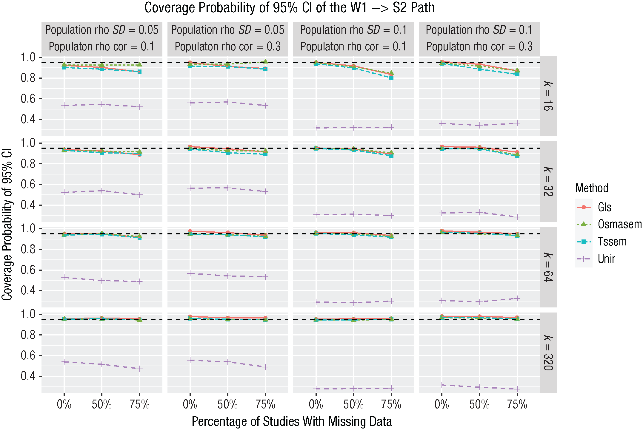
Coverage probabilities of the 95% confidence intervals of the cross paths (W1→S2 and S1→W2) in Stimulation Study 1. GLS = generalized least squares; OSMASEM = one-stage meta-analytic structural equation modeling; TSSEM = two-stage structural equation modeling; UNIR = univariate-r. The dotted black line represents the expected coverage (95%).

Simulation Study 1: discussion

This simulation study showed that all multivariate methods generally performed well in terms of model testing and estimating parameters, standard errors, and coverage of the 95% CIs. For the univariate method, the test statistic was seriously inflated, and the standard errors were heavily underestimated, leading to extreme undercoverage of the 95% CIs. The performance of the univariate-r method was bad overall and not convincingly influenced by number of studies, the correlation between random effects, or the amount of missing data. However, the amount of population heterogeneity had a large influence; large heterogeneity led to more biased results of the univariate-r method. The univariate-r method does not take heterogeneity of the correlation coefficients into account when estimating the SEM parameters, which explains this result. Even though we used a random-effects model to construct the pooled correlation matrix at Stage 1, the precision of the estimated correlation matrix was ignored at Stage 2 by simply fitting the SEM to the pooled correlation matrix, as if the pooled correlations were obtained from one big sample (with the harmonic mean of the total sample sizes across cells as the number of observations).

There were slight differences between the multivariate methods. Although the results of TSSEM and one-stage MASEM were essentially the same, the standard errors obtained using GLS were consistently larger than those obtained using TSSEM or one-stage MASEM. The standard errors of GLS were slightly overestimated in conditions with large numbers of studies, whereas the standard errors of TSSEM and one-stage MASEM were slightly underestimated in conditions with k = 16 studies.

Simulation Study 2: population model

The data-generating model with population parameter values for the second simulation study were based on the parameter estimates found by Boer et al. (2016) and are shown in Figure 8. The population values for the correlation between organizational commitment and leader effectiveness and the regression of leader effectiveness on leader-member exchange were zero. These parameters were fixed to zero in the fitted models, so that we were fitting a correct overidentified model with 2 df. The sample sizes per individual study were chosen to be identical to the sample sizes in the data from Boer et al.

Fig. 8.

The hypothesized path model of Boer et al. (2016) with the population parameter values used in the Simulation Study 2.

Simulation Study 2: method

We varied the following factors in the simulation study.

Number of studies

Boer et al. (2016) analyzed data from 132 studies, which is a relatively large number. In practice, researchers may often include fewer studies in their MASEM analysis, so we considered conditions with 100, 50, and 30 studies; within-studies sample sizes were randomly sampled from the 132 studies.

Missing data

The data-generating model in this study contains five observed variables. With more variables of interest, the probability of missing variables increases. Therefore, in this study, we evaluated conditions in which either 40% or 60% of the studies provided incomplete data. Within these studies, either 40% or 60% of the variables (two or three correlation coefficients) were missing. Missingness was imposed at random so that the missing completely at random assumption holds.

Heterogeneity

Similarly to Simulation Study 1, we set the between-studies standard deviations at .05 or .10. The correlations between the random effects were .10 or .30.

Crossing these factors produced 3 × 2 × 2 × 2 = 24 conditions. In each condition, we generated 1,000 meta-analytic data sets. We evaluated the performance of the univariate-r method, the GLS method, TSSEM, and one-stage MASEM when fitting the correct model to each of the data sets.

Simulation Study 2: results

Most replications led to converged solutions. The TSSEM approach had a few nonconvergent solutions (maximum = 18%, Mdn = 1%) when the number of studies was small (k = 30).

Performance of the test statistics

Across replications, the test statistic was expected to have a mean of 2 across replications and to be larger than the critical value in 5% of the cases. For the multivariate methods, the test statistic indeed had a mean of around 2 in all conditions. For the univariate-r method, the mean was far above 2 in all conditions, varying from 9.04 to 40.17. Consequently, the rejection percentages of the test statistic (depicted in Fig. 9) were highly inflated for the univariate-r method; rejection percentages were almost over 50% in all conditions (range = 45.18%–86.04%).

Fig. 9.

Rejection percentages of the test statistic in Simulation Study 2. GLS = generalized least squares; OSMASEM = one-stage meta-analytic structural equation modeling; TSSEM = two-stage structural equation modeling; UNIR = univariate-r. Cells shaded gray contain values considered extreme (> 10%).

The multivariate methods generally showed rejection percentages around 5%. With the smaller number of studies (k = 30), rejection percentages were a bit higher than 5% (mostly around 6% to 7%). In the k = 100 conditions, rejection percentages were generally 5% or lower. And in the k = 50 conditions, the rejection percentages were around 6% with small heterogeneity and around 5% with larger heterogeneity (SD = .1). Overall, the rejection percentages of GLS were somewhat lower than those of TSSEM and one-stage MASEM.

Bias in parameter estimates and standard errors

All methods lead to unbiased point estimates of the path coefficients. The multivariate methods generally also resulted in unbiased standard errors, whereas the standard errors of the univariate-r method were much too low. Because this finding was consistent across parameters, we present only the results for the effect of transformational leadership on job satisfaction (for results regarding the other parameters, see the supplementary materials on OSF). As shown in Figure 10, standard-error bias was extreme for the univariate-r method in all conditions. The smallest bias with the univariate-r method was −60%. The largest bias was found in the conditions with the most missing data, in which the standard errors of the univariate-r method were underestimated by around 80%.

Fig. 10.

Percentages of relative bias in standard errors of the effect of transformational leadership on job satisfaction in Simulation Study 2. GLS = generalized least squares; OSMASEM = one-stage meta-analytic structural equation modeling; TSSEM = two-stage structural equation modeling; UNIR = univariate-r. The dotted black lines indicate the range of acceptable bias (ranging from –10% to 10%).

The multivariate methods performed quite similarly, with almost identical results for TSSEM and one-stage MASEM. The standard errors of GLS were always slightly larger than those obtained with TSSEM and one-stage MASEM. This resulted in standard-error bias higher than the tolerated 10% for some conditions with cor = 0.3 for GLS.

Coverage probability of the 95% CIs

The coverage probabilities of the 95% CIs based on the estimated standard errors are shown in Figure 11. The coverage percentages for the univariate-r method are far below 95% in all conditions (around 30% to 60%), and they are close to the expected 95% for the multivariate methods. The pattern across conditions matches the results of the standard-error bias.

Fig. 11.

Coverage probability for the effect of transformational leadership on job satisfaction in Simulation Study 2. GLS = generalized least squares; OSMASEM = one-stage meta-analytic structural equation modeling; TSSEM = two-stage structural equation modeling; UNIR = univariate-r. The dotted black line represents the expected coverage (95%).

Simulation Study 2: discussion

This simulation study corroborates the findings of Simulation Study 1, showing that the statistical inferences obtained with the univariate-r method are not accurate. The test statistics were seriously inflated. The standard errors obtained with univariate-r were far too small, leading to inaccurate CIs around parameter estimates. The multivariate methods generally performed well, with slightly better standard errors for TSSEM and one-stage MASEM than those obtained using GLS.

General Discussion

Key findings

Our reanalyses of empirical data sets showed that MASEM results could be qualitatively different across different MASEM methods. Different substantive conclusions may be drawn depending on which methods were used. Our simulation study showed that the point estimates were unbiased for all evaluated methods. However, the univariate-r method for MASEM leads to biased (underestimated) standard errors for all parameters and inflated test statistics in all conditions. This is in line with earlier simulation studies comparing the univariate-r method and the multivariate methods in the fixed-effects framework (M. W.-L. Cheung & Chan, 2005; Furlow & Beretvas, 2005; Jak & Cheung, 2018). The three multivariate methods led to very similar results: GLS performed slightly better with fewer studies, and TSSEM and one-stage MASEM performed marginally better with a larger number of studies (k > 30). This is also in line with an earlier simulation study (Jak & Cheung, 2020).

As mentioned in the introduction, the bias in the standard errors for univariate-r has several causes. First, sampling covariances between correlation coefficients are ignored. Second, study-level heterogeneity is ignored when fitting the SEM. Third, differences in the precision of different elements in the correlation matrix are ignored when fitting the SEM. The first two issues logically lead to standard errors that are too small, whereas the third issue could either underestimate or overestimate the actual values of standard errors for different coefficients in the same model. Our finding of negative bias in the standard errors obtained with univariate-r is mainly provoked by ignoring sampling covariance and between-studies variances. This study showed that the choice between MASEM methods is not arbitrary. We hope the current study will motivate researchers to use multivariate MASEM methods for future studies. The univariate-r method has long been the easiest to apply because it uses standard software for meta-analysis and SEMs. However, we hope this is changing with the development of tutorial articles and user-friendly software and web applications that can assist researchers in applying multivariate MASEM (e.g., see Jak et al., 2021; Valentine et al., 2022).

MASEM with missing data or small samples

Yet another reason for the rather slow adoption of multivariate methods may be the existence of various possible misconceptions surrounding how multivariate MASEM methods deal with missing data. We discuss four issues below.

Does multivariate MASEM need at least one study with a complete correlation matrix?

Some researchers wrote that to perform multivariate MASEM, complete correlation matrices are needed in each study or at least one complete correlation matrix in one study (e.g., see Landis, 2013; J. J. Yu et al., 2016). This is a misconception. Actually, none of the multivariate methods needs a study that provides a complete correlation matrix (for an application and data set, see Schutte et al., 2021). The multivariate methods can also be applied when each study provides a single correlation coefficient such that the data are actually univariate. Simulation Study 3 reported on the OSF website provides evidence in conditions with 100% missing data—each study provided only a single correlation coefficient. The univariate-r method still failed in all these conditions; its model test statistic was seriously inflated, and it led to grossly underestimated standard errors and very poor coverage of the CIs. Meanwhile, the multivariate methods performed well. These results also show that the poor performance of the univariate-r method was not simply due to the method being univariate (not accounting for sampling covariances). The poor performance in these conditions was because the precision of the estimated correlation matrix was not accounted for when fitting the SEM, which leads to negatively biased standard errors of the SEM parameters in conditions in which population heterogeneity is larger than zero. The univariate-r method still does not perform well in conditions without heterogeneity and without sampling covariance because the univariate-r method does not account for sampling variability in the observed correlation coefficients (i.e., differences in the precision of the estimates from Stage 1 are not taken into account when using the harmonic mean of the total sample sizes across the elements in the meta-analytic correlation matrix as the sample size when fitting the SEM). As a result, the standard errors of the Stage 2 parameters are too small for some effects and too large for others (see Jak & Cheung, 2018). Therefore, missing data never justifies using the univariate-r method instead of multivariate methods, which do account for heterogeneity, sampling covariance, and differences in sampling variability across correlation coefficients.

Using synthesized correlations from previous meta-analyses in MASEM

Sometimes researchers cannot easily find primary studies reporting on some of the bivariate relationships of interest, leading to “empty cells” in the pooled correlation matrix. Bergh et al. (2016) and Viswesvaran and Ones (1995) discussed some strategies to handle this issue. One popular choice is to fill these empty cells with estimates from previous meta-analyses. This is known as the secondary use of (one’s own and existing) meta-analytic data (see Oh, 2020). Others have data about all cells in the correlation matrix but also decide to use the results from previous meta-analyses in the MASEM (see Sheng et al., 2016). Researchers then plug in the meta-analytic estimate and some sample size (e.g., the median sample size in that meta-analysis) in the MASEM as if it were obtained from a single study. By doing this, the heterogeneity in effect sizes leading to the meta-analytic estimate is ignored. Even if the meta-analytic estimate is accurate, ignoring the heterogeneity will likely lead to biased standard errors. Therefore, we advise against using meta-analytic estimates as if they were obtained from a single study. Instead, researchers should try to get the data from the individual studies included in the meta-analysis either by requesting the data from the authors of that meta-analysis or by extracting the data from the primary studies.

Will the results of the various MASEM methods converge with large numbers of studies?

In statistics, having a large sample size sometimes mitigates the negative effects of failing to meet model assumptions. For example, the normality assumption in many linear models can be relaxed if the sample size is large enough. This is not the case for the performance of the univariate-r method. Our Simulation Study 1 showed that the univariate-r method performs poorly regardless of the number of studies included in the meta-analysis. That is, even increasing the number of studies to 320, which is extremely large for MASEM, did not improve the performance of the univariate-r method.

Missing data not at random in MASEM

Data are missing data not at random (MNAR) in MASEM if the missingness of the data is related to the actual values of the missing correlation coefficients. For example, researchers may report only the large correlation coefficients and not the smaller correlation coefficients, or journals may publish articles depending on the size or significance of the effect sizes. Given the existence of publication bias, it is quite likely that some data in actual meta-analyses are MNAR. Indeed, all MASEM methods suffer from data MNAR, but the problems could be more severe for the univariate-r method compared with the multivariate methods (Furlow & Beretvas, 2005; Jak & Cheung, 2020). Both TSSEM and one-stage MASEM use the full information maximum likelihood (FIML) estimation method to handle missing data; the univariate-r method uses pairwise deletion. Empirical evidence suggests that the FIML estimation method produces less bias than pairwise deletion (e.g., Enders, 2010). In fact, the effect of MNAR on the performance of univariate-r only adds more to the detrimental effects of not taking heterogeneity, sampling covariance, or sampling variability into account.

Limitations and future studies

Our simulation study evaluated three multivariate MASEM methods based on frequentist statistics. There also exist two Bayesian multivariate MASEM methods. The first method, developed by Ke et al. (2019), has the advantages that it provides estimates of the heterogeneity of the SEM parameters itself (instead of the heterogeneity of correlation coefficients). The second method, developed by Uanhoro (2023), quantifies so-called “adventitious error” (Wu & Browne, 2015), which is defined as error resulting from differences between the general population for which a theory is hypothesized and the specific population from which observations are made. Both of these Bayesian MASEM methods take into account sampling covariance and between-studies heterogeneity, and therefore, we expect that both methods outperform univariate-r. We did not include these methods in our study because these Bayesian models are far more challenging to specify and evaluate than frequentist MASEM methods, but we encourage researchers to conduct such a simulation study in the future.

Our study was limited to evaluating the univariate-r method in the way it is most often applied in practice. Alternative ways of applying the univariate-r method include using weighted least squares at Stage 2 with a weight matrix constructed based on the univariate meta-analyses. This was done by Jak and Cheung (2018) in the fixed-effect framework wherein the weight matrix was a matrix with the inversed sampling variances of the univariately pooled correlation coefficients on the diagonal. They also evaluated univariate-r with proper constraints on the diagonal of the model-implied correlation matrix. Both adjustments indeed led to slightly better performance of the univariate-r approach (compared with how we implemented it in the present study), but the standard errors at Stage 2 were still severely biased.

In addition to research questions that are tested by fitting an SEM to the average correlation matrix, researchers may also want to test for moderating effects. For example, researchers may want to compare the sizes of direct effects in a path model across studies from different countries or across different levels of some continuous study-level variable. We did not consider moderator tests in the current study, but they can be evaluated with the multivariate methods. TSSEM and GLS allow for testing moderator effects of categorical study-level variables by creating subgroups of studies and testing the equality of SEM parameters across subgroups. However, continuous moderating variables cannot be analyzed with GLS or TSSEM (unless the continuous variable is categorized, but this is not recommended). One-stage MASEM is the most versatile method because it can evaluate the effect of continuous moderators and categorical moderators without creating subgroups.

The conclusions from a simulation study are generalizable only to the conditions that are considered in the simulation study. Despite the thoroughness of our simulation, there are still factors and conditions that have not been explored. Future studies involving the multivariate methods may be done to get more insight into the performance of the MASEM method under different conditions, such as with more complex path models. A MASEM analysis to evaluate the structure of some measurement instrument using data from different studies typically has more variables and less missing data. For example, Fong et al. (2023) obtained data from 86 studies reporting on 10 indicators of the Learning and Study Strategies Inventory, for which more than 70 of the studies provided complete correlation matrices across the 10 indicators. Additional simulations would be useful to evaluate the performance of the multivariate methods under similar data conditions. Given the inherent problems of the univariate-r method, we do not expect there to be any realistic condition in which the univariate-r method outperforms the multivariate methods.

Conclusion

Our simulation studies show that the parameter estimates of all MASEM methods including the univariate-r method are unbiased. However, the univariate-r method leads to biased statistical inferences including model testing and uncertainty estimation with standard errors or CIs. We therefore recommend using multivariate MASEM for future studies.

Footnotes

Appendix A

Here, we provide a more detailed explanation of the four meta-analytic structural equation modeling (MASEM) methods that we applied in this study.

Acknowledgements

Part of this research was presented at the 12th Annual Meeting of the Society of Research Synthesis Methodology in Montreal, Canada in 2017 and at the Webinar series of the AERA SRMA Special Interest Group in December 2021.

Transparency

Action Editor: Yasemin Kisbu-Sakarya

Editor: David A. Sbarra

Author Contributions

Suzanne Jak: Conceptualization; Data curation; Formal analysis; Funding acquisition; Investigation; Methodology; Project administration; Resources; Software; Visualization; Writing – original draft; Writing – review & editing.

Mike W.-L. Cheung: Conceptualization; Data curation; Formal analysis; Funding acquisition; Investigation; Methodology; Project administration; Resources; Software; Visualization; Writing – original draft; Writing – review & editing.

ORCID iDs

Suzanne Jak

Mike W.-L. Cheung

Notes

References

Archakov

Hansen

P. R.

Luo

(2024). A new method for generating random correlation matrices. The Econometrics Journal, 27(20), 188–212. https://doi.org/10.1093/ectj/utad027

Badura

K. L.

Grijalva

Galvin

B. M.

Owens

B. P.

Joseph

D. L.

(2020). Motivation to lead: A meta-analysis and distal-proximal model of motivation and leadership. Journal of Applied Psychology, 105(4), 331–354. https://doi.org/10.1037/apl0000439

Badura

K. L.

Grijalva

Newman

D. A.

Yan

T. T.

Jeon

(2018). Gender and leadership emergence: A meta-analysis and explanatory model. Personnel Psychology, 71(3), 335–367. https://doi.org/10.1111/peps.12266

Becker

B. J.

(1992). Using results from replicated studies to estimate linear models. Journal of Educational Statistics, 17(4), 341–362. https://doi.org/10.3102/10769986017004341

Becker

B. J.

(1995). Corrections to “Using results from replicated studies to estimate linear models.” Journal of Educational and Behavioral Statistics, 20(1), 100–102. https://doi.org/10.2307/1165390

Becker

B. J.

Aloe

A. M.

Cheung

M. W.-L.

(2020). Meta-analysis of correlation matrices and structural equation models. In Schmid

C. H.

Stijnen

White

I. R.

(Eds.), Handbook of meta-analysis (pp. 347–369). Chapman and Hall/CRC. https://doi.org/10.1201/9781315119403

Bennett

A. A.

Bakker

A. B.

Field

J. G.

(2018). Recovery from work-related effort: A meta-analysis. Journal of Organizational Behavior, 39(3), 262–275. https://doi.org/10.1002/job.2217

Bentler

P. M.

Lee

S.-Y.

(1983). Covariance structures under polynomial constraints: Applications to correlation and alpha-type structural models. Journal of Educational and Behavioral Statistics, 8(3), 207–222. https://doi.org/10.3102/10769986008003207

Bergh

D. D.

Aguinis

Heavey

Ketchen

D. J.

Boyd

B. K.

Lau

C. L. L.

Joo

(2016). Using meta-analytic structural equation modeling to advance strategic management research: Guidelines and an empirical illustration via the strategic leadership-performance relationship. Strategic Management Journal, 37(3), 477–497. https://doi.org/10.1002/smj.2338

10.

Boer

Deinert

Homan

A. C.

Voelpel

S. C.

(2016). Revisiting the mediating role of leader-member exchange in transformational leadership: The differential impact model. European Journal of Work and Organizational Psychology, 25(6), 883–899.

11.

Bosco

F. A.

Aguinis

Singh

Field

J. G.

Pierce

C. A.

(2015). Correlational effect size benchmarks. Journal of Applied Psychology, 100(2), 431–449.

12.

Browne

M. W.

(1984). Asymptotically distribution-free methods for the analysis of covariance structures. British Journal of Mathematical and Statistical Psychology, 37(1), 62–83.

13.

Chamberlin

Newton

D. W.

LePine

J. A.

(2018). A meta-analysis of empowerment and voice as transmitters of high-performance managerial practices to job performance. Journal of Organizational Behavior, 39(10), 1296–1313. https://doi.org/10.1002/job.2295

14.

Cheung

M. W.-L.

(2014). Fixed- and random-effects meta-analytic structural equation modeling: Examples and analyses in R. Behavior Research Methods, 46(1), 29–40. https://doi.org/10.3758/s13428-013-0361-y

15.

Cheung

M. W.-L.

(2015). Meta-analysis: A structural equation modeling approach. John Wiley & Sons. https://doi.org/10.1002/9781118957813

16.

Cheung

M. W.-L.

(2018). Issues in solving the problem of effect size heterogeneity in meta-analytic structural equation modeling: A commentary and simulation study on Yu, Downes, Carter, and O’Boyle (2016). Journal of Applied Psychology, 103(7), 787–803. https://doi.org/10.1037/apl0000284

17.

Cheung

M. W.-L.

(2019). Some reflections on combining meta-analysis and structural equation modeling. Research Synthesis Methods, 10(1), 15–22. https://doi.org/10.1002/jrsm.1321

18.

Cheung

M. W.-L.

Chan

(2005). Meta-analytic structural equation modeling: A two-stage approach. Psychological Methods, 10(1), 40–64. https://doi.org/10.1037/1082-989X.10.1.40

19.

Cheung

S. F.

(2000). Examining solutions to two practical issues in meta-analysis: Dependent correlations and missing data in correlation matrices [Unpublished doctoral dissertation]. Chinese University of Hong Kong.

20.

Chung

Zhan

Noe

R. A.

Jiang

(2022). Is it time to update and expand training motivation theory? A meta-analytic review of training motivation research in the 21st century. Journal of Applied Psychology, 107(7), 1150–1179. https://doi.org/10.1037/apl0000901

21.

Connelly

B. L.

Crook

T. R.

Combs

J. G.

Ketchen

D. J.

Jr Aguinis

(2018). Competence-and integrity-based trust in interorganizational relationships: Which matters more? Journal of Management, 44(3), 919–945. https://doi.org/10.1177/0149206315596813

22.

Cudeck

(1989). Analysis of correlation matrices using covariance structure models. Psychological Bulletin, 105(2), 317–327. https://doi.org/10.1037/0033-2909.105.2.317

23.

Dhanani

L. Y.

Beus

J. M.

Joseph

D. L.

(2018). Workplace discrimination: A meta-analytic extension, critique, and future research agenda. Personnel Psychology, 71(2), 147–179. https://doi.org/10.1111/peps.12254

24.

D’Oria

Crook

T. R.

Ketchen

D. J.

Jr Sirmon

D. G.

Wright

(2021). The evolution of resource-based inquiry: A review and meta-analytic integration of the strategic resources–actions–performance pathway. Journal of Management, 47(6), 1383–1429. https://doi.org/10.1177/0149206321994182

25.

Downes

P. E.

Reeves

C. J.

McCormick

B. W.

Boswell

W. R.

Butts

M. M.

(2021). Incorporating job demand variability into job demands theory: A meta-analysis. Journal of Management, 47(6), 1630–1656. https://doi.org/10.1177/0149206320916767

26.

Ellen

B. P.

III Alexander

K. C.

Mackey

J. D.

McAllister

C. P.

Carson

J. E.

(2021). Portrait of a workplace deviant: A clearer picture of the Big Five and Dark Triad as predictors of workplace deviance. Journal of Applied Psychology, 106(12), 1950–1961. https://doi.org/10.1037/apl0000880

27.

Enders

C. K.

(2010). Applied missing data analysis. The Guilford Press.

28.

Fang

Zhang

Shaw

J. D.

(2021). Gender and social network brokerage: A meta-analysis and field investigation. Journal of Applied Psychology, 106(11), 1630–1654. https://doi.org/10.1037/apl0000841

29.

Fong

C. J.

Lee

Krou

M. R.

Hoff

M. A.

Johnston-Ashton

Gonzales

Beretvas

S. N.

(2023). Meta-analyzing the factor structure of the Learning and Study Strategies Inventory. The Journal of Experimental Education, 91(2), 380–400.

30.

Furlow

C. F.

Beretvas

S. N.

(2005). Meta-analytic methods of pooling correlation matrices for structural equation modeling under different patterns of missing data. Psychological Methods, 10(2), 227–254. https://doi.org/10.1037/1082-989X.10.2.227

31.

Gnambs

Sengewald

M.-A.

(2023). Meta-analytic structural equation modeling with fallible measurements. Zeitschrift für Psychologie, 231(1), 39–52. https://doi.org/10.1027/2151-2604/a000511

32.

Gonzalez-Mulé

S. Cockburn

W. McCormick

Zhao

. (2020). Team tenure and team performance: A meta-analysis and process model. Personnel Psychology, 73(1), 151–198. https://doi.org/10.1111/peps.12319

33.

Greco

L. M.

Porck

J. P.

Walter

S. L.

Scrimpshire

A. J.

Zabinski

A. M.

(2022). A meta-analytic review of identification at work: Relative contribution of team, organizational, and professional identification. Journal of Applied Psychology, 107(5), 795–830. https://doi.org/10.1037/apl0000941

34.

Greer

L. L.

de Jong

B. A.

Schouten

M. E.

Dannals

J. E.

(2018). Why and when hierarchy impacts team effectiveness: A meta-analytic integration. Journal of Applied Psychology, 103(6), 591–613. https://doi.org/10.1037/apl0000291

35.

Harari

Swider

B. W.

Steed

L. B.

Breidenthal

A. P.

(2018). Is perfect good? A meta-analysis of perfectionism in the workplace. Journal of Applied Psychology, 103(10), 1121–1144. https://doi.org/10.1037/apl0000324

36.

Harari

M. B.

Reaves

A. C.

Beane

D. A.

Laginess

A. J.

Viswesvaran

(2018). Personality and expatriate adjustment: A meta-analysis. Journal of Occupational and Organizational Psychology, 91(3), 486–517. https://doi.org/10.1111/joop.12215

37.

Harari

M. B.

Williams

E. A.

Castro

S. L.

Brant

K. K.

(2021). Self-leadership: A meta-analysis of over two decades of research. Journal of Occupational and Organizational Psychology, 94(4), 890–923. https://doi.org/10.1111/joop.12365

38.

Hartnell

C. A.

A. Y.

Kinicki

A. J.

Choi

Karam

E. P.

(2019). A meta-analytic test of organizational culture’s association with elements of an organization’s system and its relative predictive validity on organizational outcomes. Journal of Applied Psychology, 104(6), 832–850. https://doi.org/10.1037/apl0000380

39.

Henderson

A. A.

Horan

K. A.

(2021). A meta-analysis of sleep and work performance: An examination of moderators and mediators. Journal of Organizational Behavior, 42(1), 1–19. https://doi.org/10.1002/job.2486

40.

Hoch

J. E.

Bommer

W. H.

Dulebohn

J. H.

(2018). Do ethical, authentic, and servant leadership explain variance above and beyond transformational leadership? A meta-analysis. Journal of Management, 44(2), 501–529. https://doi.org/10.1177/0149206316665461

41.

Hoogland

J. J.

Boomsma

(1998). Robustness studies in covariance structure modeling an overview and a meta-analysis. Sociological Methods & Research, 26(3), 329–367. https://doi.org/10.1177/0049124198026003003

42.

Howard

Cogswell

Smith

(2020). The antecedents and outcomes of workplace ostracism. Journal of Applied Psychology, 105(6), 577–596. https://doi.org/10.1037/apl0000453

43.

Hunter

J. E.

Schmidt

F. L.

(2004). Methods of meta-analysis: Correcting error and bias in research findings. Sage.

44.

Jak

(2015). Meta-analytic structural equation modelling. Springer. https://doi.org/10.1007/978-3-319-27174-3

45.

Jak

Cheung

M. W.-L.

(2018). Accounting for missing correlation coefficients in fixed-effects meta-analytic structural equation modeling. Multivariate Behavioral Research, 53(1), 1–14.

46.

Jak

Cheung

M. W.-L.

(2020). Meta-analytic structural equation modeling with moderating effects on SEM parameters. Psychological Methods, 25(4), 430–455.

47.

Jak

Kolbe

de Jonge

Cheung

M. W.-L.

(2021). Meta-analytic structural equation modeling made easy: A tutorial and web application for one-stage MASEM. Research Synthesis Methods, 12(5), 590–606.

48.

Jiang

Lavaysse

L. M.

(2018). Cognitive and affective job insecurity: A meta-analysis and a primary study. Journal of Management, 44(6), 2307–2342. https://doi.org/10.1177/0149206318773853

49.

Jiang

Lawrence

(2022). Does a stick work? A meta-analytic examination of curvilinear relationships between job insecurity and employee workplace behaviors. Journal of Organizational Behavior, 43(8), 1410–1445. https://doi.org/10.1002/job.2652

50.

Zhang

Tong

(2019). Bayesian meta-analytic SEM: A one-stage approach to modeling between-studies heterogeneity in structural parameters. Structural Equation Modeling: A Multidisciplinary Journal, 26(3), 348–370.

51.

Kleine

A. K.

Rudolph

C. W.

Zacher

(2019). Thriving at work: A meta-analysis. Journal of Organizational Behavior, 40(9–10), 973–999. https://doi.org/10.1002/job.2375

52.

Kleine

A. K.

Schmitt

Wisse

(2021). Students' career exploration: A meta-analysis. Journal of Vocational Behavior, 131, Article 103645. https://doi.org/10.1016/j.jvb.2021.103645

53.

Koh

Lee

Joshi

(2019). Transformational leadership and creativity: A meta-analytic review and identification of an integrated model. Journal of Organizational Behavior, 40(6), 625–650. https://doi.org/10.1002/job.2355

54.

Kooij

D. T. A. M.

Kanfer

Betts

Rudolph

C. W.

(2018). Future time perspective: A systematic review and meta-analysis. Journal of Applied Psychology, 103(8), 867–893. https://doi.org/10.1037/apl0000306

55.

Landis

R. S.

(2013). Successfully combining meta-analysis and structural equation modeling: Recommendations and strategies. Journal of Business and Psychology, 28(3), 251–261. https://doi.org/10.1007/s10869-013-9285-x

56.

Lapierre

L. M.

Kwan

H. K.

Greenhaus

J. H.

DiRenzo

M. S.

Shao

(2018). A meta-analysis of the antecedents of work–family enrichment. Journal of Organizational Behavior, 39(4), 385–401. https://doi.org/10.1002/job.2234

57.

Lee

Lyubovnikova

Tian

A. W.

Knight

(2020). Servant leadership: A meta-analytic examination of incremental contribution, moderation, and mediation. Journal of Occupational and Organizational Psychology, 93(1), 1–44. https://doi.org/10.1111/joop.12265

58.

Lee

Willis

Tian

A. W.

(2018). Empowering leadership: A meta-analytic examination of incremental contribution, mediation, and moderation. Journal of Organizational Behavior, 39(3), 306–325. https://doi.org/10.1002/job.2220

59.

Lee

Beretvas

S. N.

(2022). An evaluation of methods for meta-analytic structural equation modeling. Structural Equation Modeling: A Multidisciplinary Journal, 29(5), 703–715. https://doi.org/10.1080/10705511.2022.2047976

60.

Lee

Berry

C. M.

Gonzalez-Mulé

(2019). The importance of being humble: A meta-analysis and incremental validity analysis of the relationship between honesty-humility and job performance. Journal of Applied Psychology, 104(12), 1535–1546. https://doi.org/10.1037/apl0000421

61.

Loignon

A. C.

Woehr

D. J.

(2018). Social class in the organizational sciences: A conceptual integration and meta-analytic review. Journal of Management, 44(1), 61–88. https://doi.org/10.1177/0149206317728106

62.

Longmire

N. H.

Harrison

D. A.

(2018). Seeing their side versus feeling their pain: Differential consequences of perspective-taking and empathy at work. Journal of Applied Psychology, 103(8), 894–915. https://doi.org/10.1037/apl0000307

63.

Mackey

J. D.

McAllister

C. P.

Maher

L. P.

Wang

(2019). Leaders and followers behaving badly: A meta-analytic examination of curvilinear relationships between destructive leadership and followers’ workplace behaviors. Personnel Psychology, 72(1), 3–47. https://doi.org/10.1111/peps.12286

64.

Mesmer-Magnus

J. R.

Asencio

Seely

P. W.

DeChurch

L. A.

(2018). How organizational identity affects team functioning: The identity instrumentality hypothesis. Journal of Management, 44(4), 1530–1550. https://doi.org/10.1177/0149206315614370

65.

Michel

J. S.

Viswesvaran

Thomas

(2011). Conclusions from meta-analytic structural equation models generally do not change due to corrections for study artifacts. Research Synthesis Methods, 2(3), 174–187. https://doi.org/10.1002/jrsm.47

66.

Morris

T. P.

White

I. R.

Crowther

M. J.

(2019). Using simulation studies to evaluate statistical methods. Statistics in Medicine, 38(11), 2074–2102.

67.

T. W.

Sorensen

K. L.

Zhang

Yim

F. H.

(2019). Anger, anxiety, depression, and negative affect: Convergent or divergent? Journal of Vocational Behavior, 110, 186–202. https://doi.org/10.1016/j.jvb.2018.11.014

68.

Nohe

Meier

L. L.

Sonntag

Michel

(2015). The chicken or the egg? A meta-analysis of panel studies of the relationship between work-family conflict and strain. Journal of Applied Psychology, 100(2), 522–536.

69.

Ogunfowora

B. (T.)

Nguyen

V. Q.

Steel

Hwang

C. C.

(2022). A meta-analytic investigation of the antecedents, theoretical correlates, and consequences of moral disengagement at work. Journal of Applied Psychology, 107(5), 746–775. https://doi.org/10.1037/apl0000912

70.

I.-S.

(2020). Beyond meta-analysis: Secondary uses of meta-analytic data. Annual Review of Organizational Psychology and Organizational Behavior, 7(1), 125–153. https://doi.org/10.1146/annurev-orgpsych-012119-045006

71.

Olkin

Siotani

(1976). Asymptotic distribution of functions of a correlation matrix. In Ideka

(Ed.), Essays in probability and statistics (pp. 235–251). Shinko Tsusho.

72.

Pak

Kramer

Lee

Kim

K. J.

(2022). The impact of work hours on work-to-family enrichment and conflict through energy processes: A meta-analysis. Journal of Organizational Behavior, 43(4), 709–743. https://doi.org/10.1002/job.2595

73.

Park

H. (H.)

Wiernik

B. M.

I.-S.

Gonzalez-Mulé

Ones

D. S.

Lee

(2020). Meta-analytic five-factor model personality intercorrelations: Eeny, meeny, miney, moe, how, which, why, and where to go. Journal of Applied Psychology, 105(12), 1490–1529. https://doi.org/10.1037/apl0000476

74.

Peng

A. C.

Kim

(2020). A meta-analytic test of the differential pathways linking ethical leadership to normative conduct. Journal of Organizational Behavior, 41(4), 348–368. https://doi.org/10.1002/job.2427

75.

Pletzer

J. L.

Bentvelzen

Oostrom

J. K.

De Vries

R. E.

(2019). A meta-analysis of the relations between personality and workplace deviance: Big Five versus HEXACO. Journal of Vocational Behavior, 112, 369–383. https://doi.org/10.1016/j.jvb.2019.04.004

76.

Porter

C. M.

Woo

S. E.

Allen

D. G.

Keith

M. G.

(2019). How do instrumental and expressive network positions relate to turnover? A meta-analytic investigation. Journal of Applied Psychology, 104(4), 511–536. https://doi.org/10.1037/apl0000351

77.

Riley

R. D.

(2009). Multivariate meta-analysis: The effect of ignoring within-study correlation. Journal of the Royal Statistical Society, Series A: Statistics in Society, 172(4), 789–811.

78.

Rosopa

P. J.

Kim

(2017). Robustness of statistical inferences using linear models with meta-analytic correlation matrices. Human Resource Management Review, 27(1), 216–236. https://doi.org/10.1016/j.hrmr.2016.09.012

79.

Rubenstein

A. L.

Zhang

Morrison

H. M.

Jorgensen

D. F.

(2019). Trait expression through perceived job characteristics: A meta-analytic path model linking personality and job attitudes. Journal of Vocational Behavior, 112, 141–157. https://doi.org/10.1016/j.jvb.2019.02.002

80.

Rudolph

C. W.

Kooij

D. T.

Rauvola

R. S.

Zacher

(2018). Occupational future time perspective: A meta-analysis of antecedents and outcomes. Journal of Organizational Behavior, 39(2), 229–248. https://doi.org/10.1002/job.2264

81.

Ryu

J. W.

Neubert

E. M.

Gonzalez-Mulé

(2022). Putting the team in the driver’s seat: A meta-analysis on the what, why, and when of team autonomy’s impact on team effectiveness. Personnel Psychology, 75(2), 411–439. https://doi.org/10.1111/peps.12468

82.

Schutte

N. S.

Keng

S.-L.

Cheung

M. W.-L.

(2021). Emotional intelligence mediates the connection between mindfulness and gratitude: A meta-analytic structural equation modeling study. Mindfulness, 12(11), 2613–2623. https://doi.org/10.1007/s12671-021-01725-2

83.

Sheng

Kong

Cortina

J. M.

Hou

(2016). Analyzing matrices of meta-analytic correlations: Current practices and recommendations. Research Synthesis Methods, 7(2), 187–208.

84.

Sherf

E. N.

Parke

M. R.

Isaakyan

(2021). Distinguishing voice and silence at work: Unique relationships with perceived impact, psychological safety, and burnout. Academy of Management Journal, 64(1), 114–148. https://doi.org/10.5465/amj.2018.1428

85.

Sheu

H. B.

Lent

R. W.

Miller

M. J.

Penn

L. T.

Cusick

M. E.

Truong

N. N.

(2018). Sources of self-efficacy and outcome expectations in science, technology, engineering, and mathematics domains: A meta-analysis. Journal of Vocational Behavior, 109, 118–136. https://doi.org/10.1016/j.jvb.2018.10.003

86.

Slemp

G. R.

Field

J. G.

Cho

A. S.

(2020). A meta-analysis of autonomous and controlled forms of teacher motivation. Journal of Vocational Behavior, 121, Article 103459. https://doi.org/10.1016/j.jvb.2020.103459

87.

Song

Gnyawali

D. R.

Srivastava

M. K.

Asgari

(2018). In search of precision in absorptive capacity research: A synthesis of the literature and consolidation of findings. Journal of Management, 44(6), 2343–2374. https://doi.org/10.1177/0149206318773861

88.

Tihanyi

Aguilera

R. V.

Heugens

Van Essen

Sauerwald

Duran

Turturea

(2019). State ownership and political connections. Journal of Management, 45(6), 2293–2321. https://doi.org/10.1177/0149206318822113

89.

Uanhoro

J. O.

(2023). Hierarchical covariance estimation approach to meta-analytic structural equation modeling. Structural Equation Modeling: A Multidisciplinary Journal, 30(4), 532–546.

90.

Uanhoro

J. O.

(2024). Bayesian structural equation models of correlation matrices. Structural Equation Modeling: A Multidisciplinary Journal, 31(4), 685–695. https://doi.org/10.1080/10705511.2024.2306532

91.

Valentine

J. C.

Cheung

M. W.-L.

Smith

E. J.

Alexander

Hatton

J. M.

Hong

R. Y.

Huckaby

L. T.

Patton

S. C.

Pössel

Seely

H. D.

(2022). A primer on meta-analytic structural equation modeling: The case of depression. Prevention Science, 23(3), 346–365. https://doi.org/10.1007/s11121-021-01298-5

92.

van Hooft

E. A. J.

Kammeyer-Mueller

J. D.

Wanberg

C. R.

Kanfer

Basbug

. (2021). Job search and employment success: A quantitative review and future research agenda. Journal of Applied Psychology, 106(5), 674–713. https://doi.org/10.1037/apl0000675

93.

Vaziri

Wayne

J. H.

Casper

W. J.

Lapierre

L. M.

Greenhaus

J. H.

Amirkamali

(2022). A meta-analytic investigation of the personal and work-related antecedents of work–family balance. Journal of Organizational Behavior, 43(4), 662–692. https://doi.org/10.1002/job.2594

94.

Viswesvaran

Ones

D. S.

(1995). Theory testing: Combining psychometric meta-analysis and structural equations modeling. Personnel Psychology, 48(4), 865–885. https://doi.org/10.1111/j.1744-6570.1995.tb01784.x

95.

Browne

M. W.

(2015). Quantifying adventitious error in a covariance structure as a random effect. Psychometrika, 80, 571–600.

96.

Young

H. R.

Glerum

D. R.

Joseph

D. L.

McCord

M. A.

(2021). A meta-analysis of transactional leadership and follower performance: Double-edged effects of LMX and empowerment. Journal of Management, 47(5), 1255–1280. https://doi.org/10.1177/0149206320908646

97.

Young

H. R.

Glerum

D. R.

Wang

Joseph

D. L.

(2018). Who are the most engaged at work? A meta-analysis of personality and employee engagement. Journal of Organizational Behavior, 39(10), 1330–1346. https://doi.org/10.1002/job.2303

98.

Matta

F. K.

Cornfield

(2018). Is leader–member exchange differentiation beneficial or detrimental for group effectiveness? A meta-analytic investigation and theoretical integration. Academy of Management Journal, 61(3), 1158–1188. https://doi.org/10.5465/amj.2016.1212

99.

J. J.

Downes

P. E.

Carter

K. M.

O’Boyle

E. H.

(2016). The problem of effect size heterogeneity in meta-analytic structural equation modeling. Journal of Applied Psychology, 101(10), 1457–1473. https://doi.org/10.1037/apl0000141

100.

Zhang

Liu

Yang

L. Q.

Bednall

T. C.

(2019). Why abusive supervision impacts employee OCB and CWB: A meta-analytic review of competing mediating mechanisms. Journal of Management, 45(6), 2474–2497. https://doi.org/10.1177/0149206318823935

101.

Zhang

Liu

Zhang

Cheung

M. W. L.

(2021). Psychological ownership: A meta-analysis and comparison of multiple forms of attachment in the workplace. Journal of Management, 47(3), 745–770. https://doi.org/10.1177/0149206320917195

102.

Zhang

Jin

Ford

M. T.

(2018). The within and cross domain effects of work-family enrichment: A meta-analysis. Journal of Vocational Behavior, 104, 210–227. https://doi.org/10.1016/j.jvb.2017.11.003

103.

Zhang

T. W. H.

Lam

S. S. K.

(2019). Promotion- and prevention-focused coping: A meta-analytic examination of regulatory strategies in the work stress process. Journal of Applied Psychology, 104(10), 1296–1323. https://doi.org/10.1037/apl0000404

104.

Zhao

Chen

C. C.

Zhou

(2022). The influence of corporate social responsibility on incumbent employees: A meta-analytic investigation of the mediating and moderating mechanisms. Journal of Management, 48(1), 114–146. https://doi.org/10.1177/0149206320946108

A Cautionary Note on Using Univariate Methods for Meta-Analytic Structural Equation Modeling

Abstract

Keywords

Aim of This Study

Comparison of MASEM Methods on Empirical Data

Analyses

Results

Conclusions based on reanalyses of empirical data sets

Simulation Studies

Simulation Study 1: population model

Simulation Study 1: method

Number of studies

Missing data

Heterogeneity

Simulation Study 1: results

Performance of the test statistic

Bias in parameter estimates and standard errors

Coverage probability of the 95% CIs

Simulation Study 1: discussion

Simulation Study 2: population model

Simulation Study 2: method

Number of studies

Missing data

Heterogeneity

Simulation Study 2: results

Performance of the test statistics

Bias in parameter estimates and standard errors

Coverage probability of the 95% CIs

Simulation Study 2: discussion

General Discussion

Key findings

MASEM with missing data or small samples

Does multivariate MASEM need at least one study with a complete correlation matrix?

Using synthesized correlations from previous meta-analyses in MASEM

Will the results of the various MASEM methods converge with large numbers of studies?

Missing data not at random in MASEM

Limitations and future studies

Conclusion

Footnotes

Appendix A

Acknowledgements

Transparency

ORCID iDs

Notes

References