
Abstract
Path modeling and the extended structural equation modeling framework are in increasingly common use for statistical analysis in modern behavioral science. Path modeling, including structural equation modeling, provides a flexible means of defining complex models in a way that allows them to be easily visualized, specified, and fitted to data. Although causality cannot be determined simply by fitting a path model, researchers often use such models as representations of underlying causal-process models. Indeed, causal implications are a vital characteristic of a model’s explanatory value, but these implications are rarely examined directly. When models are hypothesized to be causal, they can be differentiated from one another by examining their causal implications as defined by a combination of the model assumptions, data, and estimation procedure. However, the implied causal relationships may not be immediately obvious to researchers, especially for intricate or long-chain causal structures (as in longitudinal panel designs). We introduce the matrix of implied causation (MIC) as a tool for easily understanding and reporting a model’s implications for the causal influence of one variable on another. With examples from the literature, we illustrate the use of MICs in model checking and experimental design. We argue that MICs should become a routine element of interpretation when models with complex causal implications are examined, and that they may provide an additional tool for differentiating among models with otherwise similar fit.
Correlations among variables in the social sciences are often consistent with a large number of potential causal models (Meehl, 1971, 1990). Path models, specifically those in the extended structural equation modeling (SEM) framework (Neale et al., 2016), are intuitive ways of relating theoretical assumptions to data and comparing theories that make substantively different predictions about the causal relations among variables.
Model fit can be evaluated in a number of quantitative ways (for a review, see Kline, 2005), but most capture the extent to which the statistical model parsimoniously reproduces the observed covariance matrix. Although fit indices are useful for model evaluation, they are not sufficient to evaluate a model’s verisimilitude. Tomarken and Waller (2003) demonstrated that models with identical fit can make strongly discrepant causal predictions. For example, structural equation models assuming the three causal structures discussed in Example 1 later in this article—the chain X → Y → Z, the chain X ← Y ← Z, and the fork X ← Y → Z (for an introduction to graphical causal models, see Rohrer, 2018)—will fit identically for any covariance matrix.
Causation in the World of Path Modeling
One of the major strengths of path-modeling approaches like SEM lies in the correspondence between the interpretable specification of the path model and the system of equations used for model fitting. The path diagram itself, with its succinct and sensible visual representation, makes it possible to quickly and easily understand the direct and indirect relations presented in the model and the flow of influence from one construct to another.
Almost since its inception, one of the apparent benefits of path modeling has been its applications for causal inference (Wright, 1934). Although a complete discussion of causality is beyond the scope of this article, a variety of sources discuss current thinking on the topic in detail (e.g., Hernán & Robins, 2020; Pearl, 2009). However, although models are frequently hypothesized to be causal, their causal implications are rarely examined.
The essence of some common conceptions of causality rests on the differences among divergent potential outcomes. For example, in Rubin’s (2004) potential-outcomes framework, the average effect of a hypothetical treatment is defined as the average difference between the observed outcome value for a particular unit if that unit received the treatment and the unit’s observed outcome value had the unit not received the treatment. Extending this idea to nonbinary sources of variation, Pearl (2009) proposed the do-calculus, according to which the causal effect of one variable on another is the change in the outcome when the explanatory variable is set to a known constant value (i.e., the effect on Y if one were to “do” X by applying an intervention that forced variable X to take value x).
Under most widely used conceptualizations of causality, experimental manipulation with a strong approximation of the counterfactual built into the research design (e.g., a randomized control group) is the strongest method for obtaining causal estimates. Thus, the usefulness of path modeling for obtaining unbiased causal estimates depends largely on the strength of the research design. However, even in the absence of a randomized experiment, SEM offers some useful affordances for causal estimation, including allowing the researcher to specify the process of selection into the causal variable of interest and to model measurement error in causal variables of interest.
Yet it is often the case that a variety of plausible statistical models with very different causal interpretations can be fitted to the same data, particularly in the absence of a strong experimental design. This presents a major challenge to researchers applying SEM to nonexperimental data. Shadish, Cook, and Campbell (2001) proposed a general set of principles, called coherent pattern matching, for obtaining causal estimates in the absence of a strong experimental design. These principles can be used to develop a set of complex predictions that differentiate among a range of plausible alternative hypotheses. For example, if a school offered some non–randomly assigned tutoring program, a partial correlation between attending that school and scores on a reading achievement test might be hypothesized to approximate the causal effect of the program on the outcome. In that case, one’s confidence in the hypothesis would be decreased if the estimate was the same when a reading pretest replaced the reading posttest as the outcome measure. Similarly, one’s confidence in the hypothesis would be reduced if similar achievement scores were observed for the students who did not participate in the tutoring program, or for students in similar schools that did not offer the program. In essence, coherent-pattern-matching principles encourage researchers to compare models on the basis of their implied causal structure.
Implied Causal Structure as a Means of Model Validation and Interpretation
We argue that understanding the causal implications of a model is an integral part of evaluating the validity of the process it implies. We encourage researchers to incorporate examination of these implications as a standard part of model evaluation, both as a means to aid interpretation and as a means of ruling out those models whose causal implications are nonsensical. For example, if X occurs after Z, the causal structure X → Y → Z contradicts the assumption that effects cannot precede their causes, and models implying such a prediction might be rejected. Even when a model is fitted to data that do not come from a randomized experiment, it may still have causal implications that can be compared with effects estimated from randomized controlled trials (e.g., Shadish, Clark, & Steiner, 2008).
A variety of tools already exist to identify different concerns related to model structure or fit. For example, researchers commonly flag cases of negative estimated variance (often called Heywood cases). A negative estimated variance can be considered sufficient to rule out a model because it conflicts with the statistical definition of variance as a nonnegative quantity. Similarly, an assumption test, such as a test of conditional independence, may be used to reject a model because of a conflict with an underlying statistical assumption. Each of these approaches quantifies some quality of models that is not captured by traditional indices of goodness of fit. This quantification in turn allows researchers to reject models on the basis of conflicts between those quantities and theoretical statistical assumptions or beliefs. In this article, we introduce a novel tool that can be used similarly: the matrix of implied causation (MIC). By quantifying the causal predictions of models, MICs provide a way to reject those whose implied causal predictions conflict with theoretical assumptions or definitions of causality. MICs therefore supplement the existing toolbox of statistical modelers and provide a new means of quickly identifying conflicts between their models and existing theory.
Similarly, some search procedures can help researchers to identify more complete or better-fitting models. For example, a researcher might use modification indices to search for places where model paths might be freed to improve statistical fit (see, e.g., Sörbom, 1989). Other tools search through large classes of models to identify sets of models that meet specific criteria. For example, the Tetrad software (Scheines, Spirtes, Glymour, Meek, & Richardson, 1998; Spirtes, Scheines, Ramsey, & Glymour, 2015) can search a large class of models to identify any that are equivalent to a given model and meet a set of specific constraints (some of which may be related to cause). SEM tree approaches (Brandmaier, von Oertzen, McArdle, & Lindenberger, 2013) similarly search for extensions of a model that differentiate independent subgroups using instrumental moderator variables. MIC tables, which we also introduce in this article, are similar in that they are useful for selecting among models. However, rather than searching through a large set of models, MIC tables present a succinct summary of the causal implications of a prespecified set of models to allow researchers to easily and directly compare a small number of candidate models in terms of their fit to a causal theory. Information from MICs may also be utilized in a variety of other ways, which we describe in more detail later in this article.
Using Implied Causal Structure to Inform Experimental Design
We suggest that the causal structures implied by a model provide an opportunity to examine the effects of different potential interventions on an outcome. Specifically, by examining the implied effects of each predictor on each outcome for a given model, it should be possible to compare possible interventions to determine the most effective ways to influence some outcome or to measure an effect on that outcome according to that model.
Implied Causal Structure as a Means of Model Comparison
We argue that the causal implications of a model also are potentially useful for adjudicating among statistically equivalent or similarly fitting models. Specifically, by evaluating models’ causal predictions with respect to logical or empirical constraints, it may be possible to select one model over another on the basis of the plausibility of the models’ causal implications. When preexisting information about these causal effects is available, one model may be clearly favored. When the existing data are not sufficiently clear, this type of comparison can be used to identify hypothetical manipulations whose implied effects on an outcome differ between the models. Implied causal structure can therefore be used to design experiments that optimally distinguish between two equivalently fitting models.
Introducing MICs
A MIC quantifies a structural equation model’s predictions about the causal effect of a hypothetical change in any variable in the model on all other variables in the model. It is nothing more than an efficient and succinct representation of the total effect (i.e., the sum of direct and indirect effects) of each variable in the model on each other variable. As a result, a MIC can be computed with almost any statistical software package. Properly applied, MICs can be used to identify model misspecifications and make testable predictions about the effects of hypothetical interventions. We argue that examination of MICs should be a standard part of model evaluation and interpretation.
The MIC computation complements Wright’s (1934) tracing rules for recovering the covariance between two variables in a structural equation model: Whereas Wright’s rules address the backward causal question, “assuming the model is true, why are X and Y correlated?” MICs allow for a direct answer to the forward causal question, “assuming the model is true, what would happen to Y if a 1-unit change in X is induced?” (for more on this distinction, see Gelman & Imbens, 2013). Judgments of verisimilitude might depend on both questions, but the latter more directly allows for the integration of quantitative information from prior work and may inform future designs that differentiate models. In this article, we describe how a MIC is calculated and how it can be obtained from a standard structural equation model. We then provide examples of MICs for published models and discuss potential misuses of MICS, as well as their limitations and avenues for future research.
Disclosures
The MICr package in R (Brick & Bailey, 2019; https://github.com/trbrick/MICr) provides functions to compute MICs and examples of how to use them using R (R Core Team, 2019) and OpenMx (Version 2.13.2; Neale et al., 2016). Some of these examples are reproduced at https://quantdev.ssri.psu.edu/tutorials. All code used in this document is available in the vignettes of that package and included in the Supplemental Material (http://journals.sagepub.com/doi/suppl/10.1177/2515245920922775). The figures were originally created using Ωnyx (von Oertzen, Brandmaier, & Tsang, 2015) and modified for readability.
Computing MICs
The path diagram associated with a traditional structural equation model is a directed acyclic graph made up of three types of nodes and two types of arrows. Square nodes represent measured manifest variables, whereas round nodes indicate unmeasured latent variables, which may be latent common causes (e.g., factors), sources of residual error, or intermediate endogenous constructs, such as “true scores” in a panel model or random effects in some other models. Triangular nodes represent intercepts or means and are not used in the computation of MICs. Paths may be represented by one-headed arrows, indicating regression predictions or causal effects, or two-headed arrows, indicating covariance due to shared causes not included in the model. Thus, one-headed arrows imply causal links, whereas two-headed arrows imply covariation in the absence of causation. 1
Single-headed arrows in a path diagram may not always describe the modeler’s causal predictions (see the discussion of potential misuses later in this article). Further, well-fitting models with significant estimated path coefficients are usually not sufficient to draw strong causal inferences in the absence of additional design features (e.g., random assignment). However, these paths are often specified to represent theorized causal links. If one assumes that all single-headed arrows are intended to be interpreted this way, one can compute the implied causal influence from a source node to a target node using a variation of Wright’s (1934) path-tracing rules.
The path-tracing rules for MICs closely resemble those put forward for the model of means: First, follow only one-headed arrows in the direction of the arrows. That is, for a path X → Y → Z, one traces the paths from X to Y and Y to Z, but not from Z to Y or to X. Second, calculate the influence along a single path as the product of all coefficients along that path. The total causal influence of one variable, C, on another, E, is the sum of the influence scores of every possible path from C to E and represents the expected difference in the target (in its native units) corresponding to a unit difference in the source. The influence along each path represents the amount of that difference that is mediated by the set of variables encountered along that path, in the order in which they appear.
For example, consider Figure 1, which depicts a traditional causal mediation structure. In this diagram, X has a direct effect on Y, indicated by the path labeled λ = 0.2, and a direct effect on Z, indicated by α = 0.8. Z, in turn, has a direct effect on Y, indicated by β = 0.6. Assuming that the effects are fully captured by these linear coefficients, the indirect effect of X on Y is α * β, or 0.48.
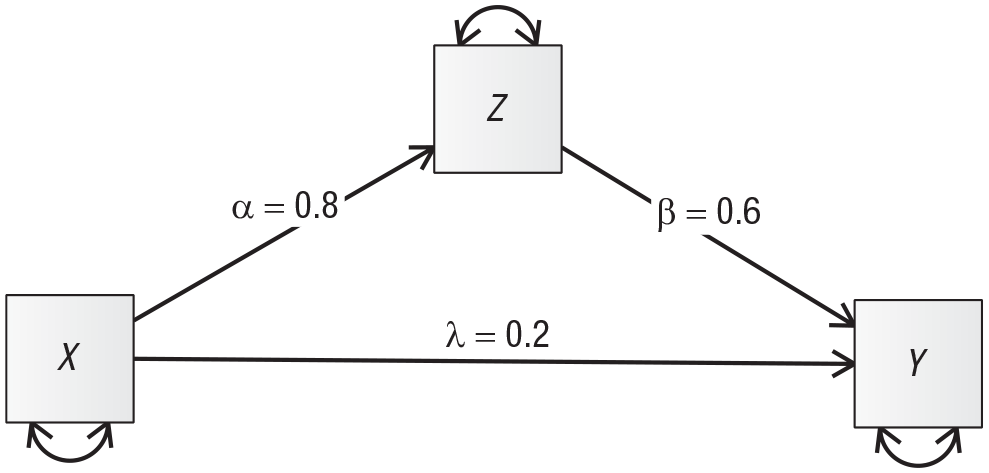
A simplified path model (specifically, a partial mediation model) depicting a theoretical causal relationship.
These same values can be quickly calculated using the path-tracing rules. The direct effect of X on Y is the sum of all one-headed arrows that travel from X to Y directly—in this case, only arrow λ. The total indirect effect mediated by Z is the sum of all paths from X to Y that go through Z (in this case, again, only one). Each indirect effect has the value of the product of the coefficients, here, α * β, or 0.48. Together, these values suggest that if all else is equal, a difference of 1 in X will result in a difference of 0.68 (i.e., 0.48 * 1 + 0.2 * 1) in Y.
Although path tracing is an excellent way to generate understanding, the same final result can be captured much more succinctly in a MIC (see Box 1 for the matrix computations): a matrix showing the implied causal effect of every variable in the model on every other. For the model displayed in Figure 1, the MIC is as follows:

Computation of a Matrix of Implied Causation From the
For a large model, the entire matrix of implied causation (MIC) can be computed quickly and efficiently using matrix algebra. We begin with the identity matrix
By multiplying

In some very rare cases, especially those using unique features of the extended structural equation modeling framework (Neale et al., 2016), the series does not converge; in that case or in the more common case when it is simply more efficient, the following equivalent formulation can be used:

The


In the MIC, element
The MIC is displayed such that element
Applications of MICs
We envision three major benefits of using MICs to investigate model structures. First, MICs directly expose the causal structures that may be obscured by complex indirect pathways. The values of the MIC cells can then be examined directly to determine whether they match the expectations according to theory or prior findings, providing a measure of face-level statistical validity, and raising potential problems of scale. Example 2 in the next section illustrates a case in which this type of surface validity can be questioned. Model selection can be informed by the models’ differing implied causal pathways, in conjunction with logic and prior research.
Second, when MICs from several models are compared, it becomes possible to identify differences in the models’ causal structures quickly and algorithmically. This is useful to inform future experimental studies in which one construct is manipulated and its causal effects directly measured, and provides a new means of model comparison when traditional fit statistics are identical or nearly identical. Example 1 illustrates a case in which the optimal choice of manipulation may not be immediately obvious.
Finally, when potential interventions are compared (e.g., for the design of a future study), MICs can provide important information about their model-implied effects on outcomes. Example 3 illustrates a comparison of three interventions whose influences can be easily quantified by a MIC.
Models’ MICs can differ in several theoretically important ways. In some cases, one model predicts a causal effect, and another does not. This situation is most informative for future studies because, when paired with a strong design, a traditional statistical test can be used to falsify one model, tentatively leaving the other under consideration. In other cases, competing models make different predictions about the sign of a causal effect. This indicates a difference in predictions that, again, paired with a strong design can be tested using one-tailed tests of the final effect. Finally, and perhaps more commonly, models may show the same directional effect, but one model may predict a larger effect than another. It is possible to differentiate models on the basis of these scale differences, although they may be heavily influenced by characteristics of the sample (e.g., for standardized effects), and power to differentiate the effects may be difficult to achieve. Note that the scales of the endpoints of a path determine the scale of the causal-influence metric independently of the scales of mediators. A MIC can be easily computed for the standardized model if standardized estimates are required, or if the scales are equivalent, quantitative differences can be examined in detail by computing approximate standard errors using the delta method (Raykov & Marcoulides, 2004) or confidence intervals via likelihood profiles (Neale & Miller, 1997). Some differences in the details of model specification (e.g., the scaling of common factors) may still influence the scale and even sign of predictions in a model, and researchers should ensure consistency in these terms whenever possible.
In the next section, we provide examples illustrating that attending to causal implications may provide insight helpful for model selection and the design of future studies.
Examples
The examples we discuss here were drawn from the literature. They show that a MIC can provide important details about the causal implications of a model and thereby inform assessments of face validity and plans for future work.
Example 1: a simplex
Tomarken and Waller (2003) thoroughly described the problem of model nonuniqueness with respect to traditional fit indices. Specifically, they presented several examples of models that fit identically but provide substantively different predictions. Here, we reproduce an example from their article to demonstrate how MICs provide differential predictions that may help to distinguish such models from one another.
The three models shown in Figure 2 are simple variations on a simplex structure. They are equivalent in their fit statistics, but they differ nontrivially in their causal structure. Table 1 clearly shows the differences in the causal structures they imply. 2
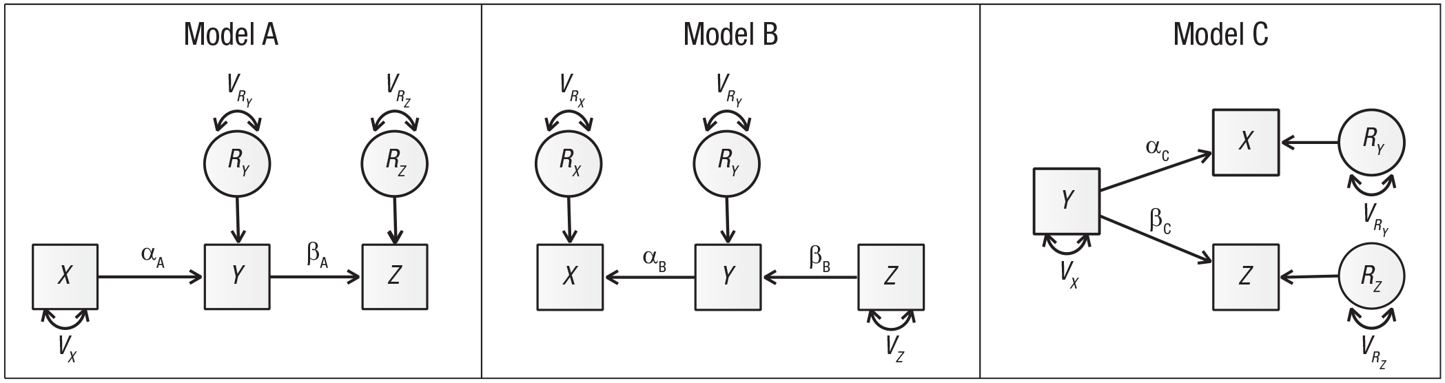
Path diagrams of three models from Tomarken and Waller (2003). These models have equivalent fit, but very different causal implications.
Matrices of Implied Causation for the Three Models in Example 1
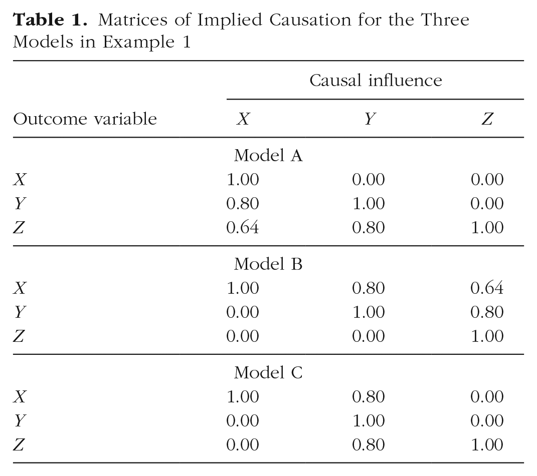
As the table shows, the three causal structures have nearly nothing in common other than the unit diagonals, even though the implied covariance matrices are identical (see Table 2). Notice that the MICs for Models A and B are transposed forms of each other—the causal influences are identical, but influence is predicted to flow in precisely the opposite directions. Model C carries a different causal structure altogether.
Model-Implied Covariance Matrix for the Three Models in Example 1
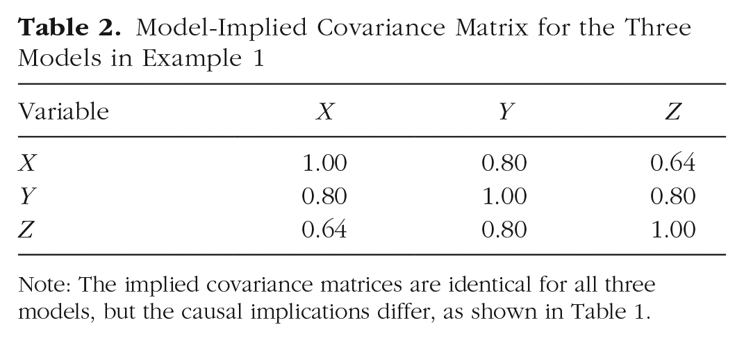
Note: The implied covariance matrices are identical for all three models, but the causal implications differ, as shown in Table 1.
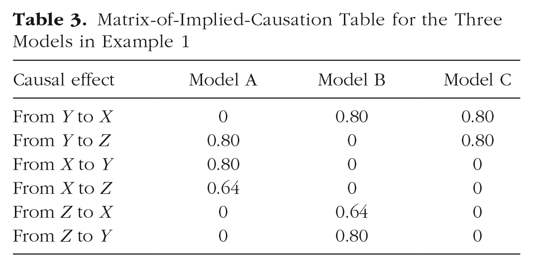
Of particular note is the ability of the MICs to identify a manipulation that will distinguish the three models. A typical research approach in this case might be to manipulate X or Z, because these represent hypothesized root causes for the chained effects. The MIC comparison table (MIC table) in Table 3 shows the causal estimates for each model and suggests a different approach. Only source Y shows a different pattern of zero and nonzero elements for each of these three models. Manipulating X will clearly differentiate Model A from the other two models. However, the total effect of X on Y and Z is identical in Models B and C, so it will be very difficult to differentiate these two models if one manipulates only X. Manipulations of Z distinguish Model B from the other models, but cannot distinguish Model A from Model C at all. All else being equal, manipulating Y will best differentiate the models.
Matrix-of-Implied-Causation Table for the Three Models in Example 1
Example 2: longitudinal analyses
Panel models are very common in the longitudinal literature, but can result in biased causal estimates when various assumptions are violated (Hamaker, Kuiper, & Grasman, 2015; Zyphur et al., 2019). Bailey, Oh, Farkas, Morgan, and Hillemeier (2019) presented a series of closely related variations on cross-lagged panel models (CLPMs) to characterize the development of math and reading achievement across the early school years. We examine the differential predictions of two types of CLPMs for an early intervention targeting children’s reading or math skills.
These models are somewhat intricate, consisting of four measurement occasions for reading and four for math, as well as up to 10 latent variables, for a total of up to 18 possible causal sources and as many possible outcomes. The first two models, dubbed 1 and 2 by Bailey and colleagues (2019), are shown in Figure 3 and represent two different views of the learning process. Model 1 is a standard CLPM and includes an autoregressive path (depicted with vertical arrows) within each domain to account for the influence of knowledge on knowledge and learning within the same domain from year to year. The model also includes cross-lagged paths (diagonal arrows) from math achievement one year to reading achievement the following year and from reading achievement one year to math achievement the following year. Further, there is residual covariation (horizontal two-headed arrows) between the test scores at each wave. The observed variables are math and reading achievement in kindergarten and Grades 1, 2, and 3.
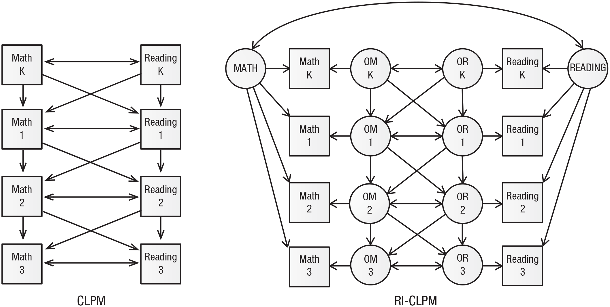
Path diagrams describing models of children’s math and reading achievement from kindergarten through third grade (adapted from Bailey, Oh, Farkas, Morgan, & Hillemeier, 2019). The cross-lagged panel model (CLPM) includes an autoregressive path within each domain, cross-lagged paths from achievement in one area to achievement in the other area the following year, and residual covariation at each wave. The random-intercept CLPM (RI-CLPM) additionally includes a random intercept for each domain and moves the autoregressive paths to the latent occasion-specific variables for reading and math achievement, labeled OR and OM, respectively. K = kindergarten; 1 = Grade 1; 2 = Grade 2; 3 = Grade 3. For clarity, variance paths are not displayed.
Model 2, a random-intercept CLPM (RI-CLPM), introduces a random intercept for each domain for each student: a non-time-varying latent skill level describing a student’s overall ability level that is independent of learning and does not change over time (labeled MATH and READING). The other factors assumed to influence achievement are domain- and occasion-specific factors (e.g., OM K for math in kindergarten and OR 1 for reading in Grade 1; see Fig. 3). As in the CLPM, each time point is part of both autoregressive and cross-lagged paths, and there is residual covariation among the occasion-specific factors at each time point, indicating that some unmeasured factors might influence both math and reading achievement in the same year.
Given that these two models have different structures, is it possible to compare their causal implications? We argue that the answer is yes, under certain assumptions. In particular, the CLPM implies that an intervention targeting reading or math in kindergarten will carry over to reading and math scores in subsequent years; however, the predictions of the RI-CLPM depend strongly on the pathway that the intervention is assumed to target. An intervention that directly targets math performance in kindergarten, for example, will not carry over to any future test score at all. By contrast, an intervention that raises math performance in kindergarten via the MATH intercept factor will have equivalent impacts on all subsequent measures of math achievement, and no impact on subsequent reading achievement. Finally, an intervention that raises math achievement in kindergarten by 1 unit via the domain- and time-specific factor OM K will influence subsequent math and reading scores via the influence of that factor on the domain- and time-specific factors for math and reading in Grade 1, OM 1 and OR 1, in a process that resembles the process modeled in the CLPM. In practice, the impacts of math interventions around school entry have been found to decay at roughly the rate implied by an autoregressive path (Bailey, Duncan, Watts, Clements, & Sarama, 2018), and it is therefore reasonable to expect that a hypothetical intervention will follow this pattern. Of course, interventions that operate via different pathways might be possible as well.
Here, we compare the model-implied causal structure of the CLPM for interventions that operate directly on achievement scores with the implied causal structure of the RI-CLPM for interventions that affect achievement scores by the same amount via the domain- and time-specific factors. The complete MIC for each model is extensive, but the MIC table can be used to easily compare noteworthy differences between the two models. Table 4 presents selected rows from the MIC table that highlight predictions about a manipulation that improves kindergarten math or reading scores by 1 unit. Specifically, the CLPM and RI-CLPM columns illustrate the two models’ predictions for the manipulation’s effects on later math and reading outcomes.
Matrix-of-Implied-Causation Table for Example 2
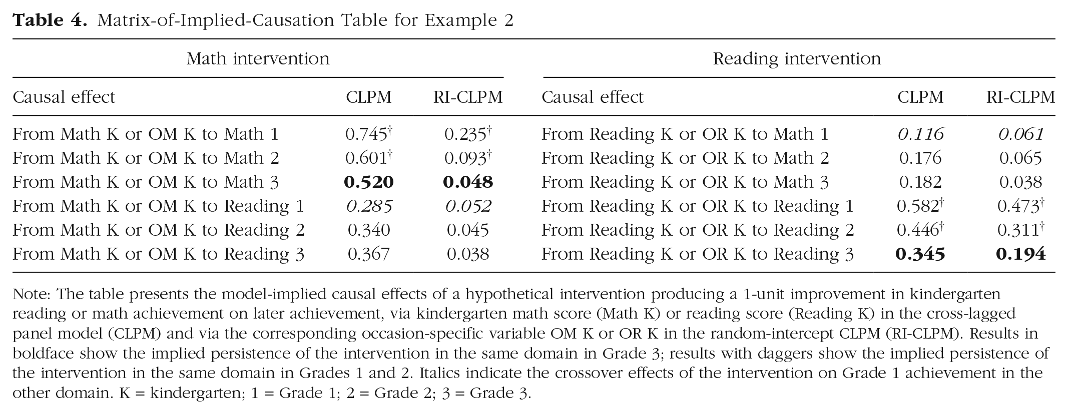
Note: The table presents the model-implied causal effects of a hypothetical intervention producing a 1-unit improvement in kindergarten reading or math achievement on later achievement, via kindergarten math score (Math K) or reading score (Reading K) in the cross-lagged panel model (CLPM) and via the corresponding occasion-specific variable OM K or OR K in the random-intercept CLPM (RI-CLPM). Results in boldface show the implied persistence of the intervention in the same domain in Grade 3; results with daggers show the implied persistence of the intervention in the same domain in Grades 1 and 2. Italics indicate the crossover effects of the intervention on Grade 1 achievement in the other domain. K = kindergarten; 1 = Grade 1; 2 = Grade 2; 3 = Grade 3.
Reading the table, one can see that the CLPM, compared with the RI-CLPM, predicts much more persistent impacts of a change to kindergarten math or reading skills on children’s math and reading skills through Grade 3. For example, a 1-unit increase in kindergarten math achievement is predicted to improve children’s math achievement in Grade 3 by 0.52 units in the CLPM, but only 0.05 units in the RI-CLPM. The predicted effects of a kindergarten reading intervention on Grade 3 reading follow a similar pattern. Another important difference is that the effects of reading on math and vice versa grow across time in the CLPM, but shrink in the RI-CLPM.
The within-domain 1- and 2-year effects on math achievement also differ broadly, ranging from 0.60 to 0.75 in the CLPM and from 0.09 to 0.24 in the RI-CLPM. In an experimental context, these estimates can be interpreted as the predicted persistence of an intervention that raises kindergarten math scores by 1 unit when math achievement is measured 1 or 2 years later. In a discussion of studies of early math interventions with follow-up assessments at least 1 year after the end of treatment, Bailey et al. (2018) reported an average 1-year persistence of approximately 0.40, and smaller values for persistence 2 years later. Jacob, Lefgren, and Sims (2010) reported 1-year persistence of teacher-induced academic improvements of between 0.20 and 0.30 in both math and reading. Although neither model exactly recovers these estimates, the CLPM appears implausible in this case, because it both overestimates these values and predicts increasing, rather than decreasing, effects as time goes on after the end of the hypothetical intervention.
Another interesting way in which these models differ in their implied causal structure is that the CLPM implies asymmetric transfer; the effect of changes to children’s kindergarten math achievement on Grade 1 reading achievement (0.29) is larger than the effects of changes to kindergarten reading achievement on Grade 1 math achievement (0.12). In the RI-CLPM, the difference between these estimates is small, trending in the opposite direction (0.05 and 0.06). Bailey et al. (2019) argued that this latter pattern is more plausible a priori, given the cognitive processes involved in math and reading.
Thus, the MIC makes predictions about the causal effects of hypothetical exogenously induced changes to variables in the model. These predictions are relevant to theoretical and practical endeavors, including intervention design, power analysis, and model selection. They can be evaluated on the basis of existing theory and parameter estimates from prior relevant experiments, but can also be used in designing experiments, which we discuss in the next section.
Example 3: experimental design
In order to precisely illustrate the use of MICs for design, we present a third example comparing the predicted effects of three different interventions according to the RI-CLPM model in Example 2. The causal structure of this model is somewhat vague because the random intercept is a catchall element representing all unmeasured between-person effects that result in systematic improvement. We discuss this point in more detail in the section on potential misuses of MICs. Because the hypothetical interventions will not be applied until after the kindergarten measurement, any intervention influencing these monolithic random intercepts would require changes to the model structure.
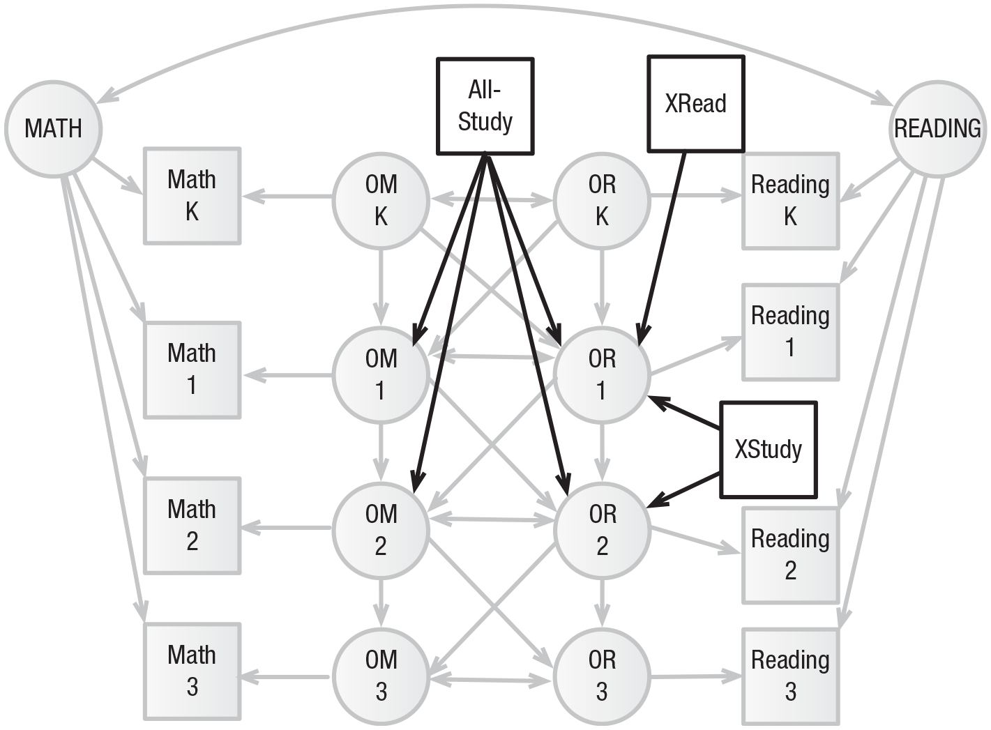
We hypothesize three interventions that might be applied at the end of kindergarten to improve reading ability. The first, a focused reading intervention called XRead, directly improves the occasion-level latent variable that influences Grade 1 reading performance; the expected improvement is 1 point. The second intervention, XStudy, focuses on study skills specific to reading across a more extended period. It is expected to improve reading scores directly by 0.5 points in first grade and by another 0.6 points in second grade. The third intervention, AllStudy, expands this intervention to include math study skills in the hopes of taking advantage of the cross-lagged associations. Because the time spent on each topic (i.e., reading vs. math) will be reduced, the expected size of the effect on each outcome is similarly reduced, to 0.4 in first grade and 0.3 in second grade. The interventions are added as additional manifest variables in Figure 4, and the MIC table showing these three interventions’ effects on third-grade reading is shown in Table 5. As the table shows, the model implies that the longer-term reading intervention, because it is subject to less autoregressive decay, is likely to be more effective than either the more intensive first-grade-only reading intervention or the longer-term reading-and-math intervention.
Matrix-of-Implied-Causation Table for Example 3
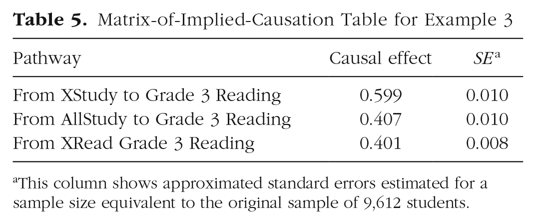
This column shows approximated standard errors estimated for a sample size equivalent to the original sample of 9,612 students.
In order to compare these different interventions directly, it could be helpful to have approximations of the expected standard errors around the estimates of the model-implied causal effects. Because the interventions are hypothetical, it is not possible to directly compute standard errors based on a fit to real data. However, by treating the model-implied covariance matrix as though it were the true population matrix, one can estimate the asymptotic standard errors for a given sample size using the delta method (Raykov & Marcoulides, 2004). Note that if there are any hypothesized interventions that have not been run (such as the ones in this example), this process requires defining a variance for each one in the structural equation model. In the current example, we set intervention variances to 0.25, which is appropriate for a balanced design and an intervention variable coded as 0 or 1, and used a sample size equal to that of the original study (N = 9,612). Standard errors computed in this way are included in Table 5. The model implies that the XStudy intervention will be nontrivially more impactful than the others, but that AllStudy and XRead are statistically indistinguishable in their effects on reading at this sample size. This same approach can be used to determine the sample size needed to distinguish these two interventions. Roughly 62,027 participants would be necessary to reduce the standard error sufficiently for these two models to be distinguished at the .05 level.
We hope that examination of the predicted causal effects of interventions will be useful in both (a) formalizing the predictions of models estimated with nonexperimental data so that these models can be more easily falsified and (b) providing predicted effect sizes that can be used in power analyses. The MICr package allows researchers to quickly compare the downstream effects of their hypothesized interventions. Additionally, if information about the cost of hypothetical interventions is available, the MICr package allows the user to identify the optimal intervention within a set of hypothetical interventions available for a given cost.
Anticipating and Avoiding Potential Misuses
We see the MIC as a potentially useful tool, but also see the potential for misinterpretation and accidental misuse. We attempt to head off these misunderstandings here.
Judging a MIC’s usefulness depends on outside information
The most important point is that a MIC must be interpreted with respect to a variety of contextual factors: It does not provide causal evidence in and of itself. Estimates in a MIC, like parameter estimates from other models that might be used in causal inference, depend on the assumptions of the model from which they were derived. Without exogenous variation (e.g., a randomly assigned treatment), cases in which any effects should be confidently interpreted as causal may be rare. MICs are intended to allow researchers to (a) generate contrasting predictions across models so as to generate potential experiments that could distinguish among them, (b) examine and compare possible interventions in terms of their predicted influence on outcomes, and (c) bring in relevant outside theoretical and empirical information—especially relevant causally informative estimates from prior research—to aid in model selection. As is always the case in statistical modeling, if all models considered are critically misspecified, it will be impossible to choose the correct model.
Not all SEM estimates are intended for causal interpretation
It is also worth noting that some paths in a structural equation model may not be intended to indicate causal relations. To decrease the bias in one path, a researcher might either induce bias in another or introduce a potentially misleading causal path into a model (Cinelli & Hazlett, 2020). For example, to estimate the causal effect of a school library program on students’ reading achievement, a researcher might regress reading achievement on a measure of the number of books in each child’s home. This might serve to increase precision in the estimated treatment effect or to reduce confounding between the home literacy environment and the program. In such a case, the path from books at home to reading achievement is unlikely to represent an unbiased estimate of the causal effect of this book count on reading achievement; it should not be used to suggest that an intervention in which children receive books but no other changes are made to the home literacy environment will improve literacy proportional to the coefficient estimated in this model. In another case, a researcher might treat a set of correlated confounds as a reflective latent variable. Although doing so may under some circumstances reduce bias in some estimates, it may also increase bias in others (Rhemtulla, van Bork, & Borsboom, 2019). It is therefore vital to be clear about which paths the researcher intends to be interpreted causally, and which are included in the model to serve some other purpose.
Integrating a MIC with statistical fit indices
Our first two examples highlight the use of MICs when traditional fit statistics are insufficient to make a clear judgment about which of a set of models is better. That is, the fit statistics of the models are either identical (as in Example 1) or nearly identical. We argue that although the causal implications of a model are especially important in these cases, they should also be taken into account in other scenarios. Specifically, we argue that even a well-fitting model should be rejected if its causal implications are either impossible or not sensible (e.g., if it implies that later events affect earlier ones), and should be questioned if its implications run counter to strong logic or evidence (e.g., Example 2).
In causal-chain or fork models, different organizations of paths among the latent structures may provide nearly identical statistical fit with different causal implications. In longitudinal and panel-style models, the same holds, although the addition or removal of unmeasured intercept, or trait, variables may be helpful. However, there may be cases in which the models with the most plausible implied causal structures do not show the strongest statistical fit, but no model’s implied causal structure is clearly impossible a priori. In such cases, the researcher must weigh a model’s statistical fit against the plausibility of its causal implications, basing this plausibility on the strongest available theory, evidence, and logic (we have not attempted to develop formal quantitative methods for doing so).
Integrating MICs and experiments requires judgment
We recommend comparing implied causal effects from experiments with MIC elements and using MICs to inform experimental design. However, if the intervention of interest does not appear in the models under consideration, both of these tasks require assumptions about the intervention. Specifically, which variables in the model are affected by the intervention? Which variables in the model are intended to represent manipulable causes? Are variables outside the model also affected by the intervention?
For example, in the RI-CLPM discussed in Examples 2 and 3, the random intercepts are usually not specifically interpreted as single causal entities, but rather represent sets of unmeasured persistent influences (e.g., biological, social, cultural, or psychological features) that lead to a child’s overall ability in a way that is stable across time. The catchall nature of these latent variables may indicate that the mechanisms that underlie them are modeled imprecisely. The causal implications of a change in these variables may provide a useful starting point for developing a more detailed theory of those mechanisms.
Some researchers may view it as possible that an intervention after kindergarten might directly increase a participant’s individual random intercept—that is, it might permanently alter those unmeasured factors that influence a child’s stable ability across time. Such an intervention is likely much different in kind from interventions that cause time-specific variations in achievement.
A researcher hypothesizing this type of change from an intervention may wish to modify the model (e.g., by adding a separate postintervention intercept), to adjust the way the impact of the intervention is construed (e.g., as having a direct effect at all time points after the intervention), or, in the best case, to clarify the model specification to more specifically show the important mechanisms being manipulated. In any of those approaches, thinking through the model’s causal implications would help to highlight this important lack of theoretical clarity and encourage the researcher to address it, for example, by placing additional focus on those causal effects susceptible to intervention or by considering alternative models that more clearly specify the theorized underlying causal processes. We argue that widespread examination of MICs during the design and evaluation of models would draw attention to their causal implications and encourage modelers to more directly confront situations in which causal structure is unclear.
Limitations and Future Work
The current work is only a beginning, and we have not explored many possible extensions. Similar models have also been presented for related cases. For example, impulse-response models have been used to examine systematic change responses in time-series network models (Yang et al., 2019). MICs do not test causality, and the standard errors reported in MIC tables should not be interpreted as indicators of a formal test of causality. Such tests are possible under some models of causality (e.g., Granger causality; see, e.g., Zyphur et al., 2019), but are beyond the scope of this article.
The current formulation of MICs was developed specifically for structural equation models in which each predictor appears only once and path parameters can be considered to be fixed effects unvarying across individuals. That is, we explicitly excluded those models in the extended SEM framework that utilize interaction terms or have multilevel structure (e.g., Pritikin, Hunter, von Oertzen, Brick, & Boker, 2017), models whose paths are composed of complex algebraic expressions (e.g., Voelkle & Oud, 2012), cases wherein variables are transformed (e.g., logistic analysis or categorical variables; e.g., Pritikin, Brick, & Neale, 2018), and others. Although some of these extensions would be trivial (e.g., a multigroup model would feature a MIC for each group); others are more complicated. We relegate these to the realm of future work.
MICs are intended to help researchers evaluate models and select from among a set of prespecified models. They cannot help researchers select the correct model if the correct model is not already under consideration. Indeed, if researchers have strong a priori evidence or beliefs about, for example, the magnitudes of a set of effects, they might reasonably reject all of the models under consideration in some cases. Similarly, the estimates of causal influence that a MIC derives from a model are measures of the model’s implications and are only as accurate to the data and its true generating process as the model from which they are derived and the causal assumptions that it makes.
Conclusions
MICs provide a simple “at a glance” view of the causal and predictive implications of any model that can be represented as a structural equation model. MIC tables allow researchers to quickly compare models and identify areas where different models make different—ideally, testable—predictions about the effects of an intervention. We have provided a series of examples to demonstrate the overall utility of MICs for understanding and interpreting models, for examining the face validity of the predictions made by a given model and its fitted values (and possibly rejecting a model on those grounds), for comparing models in terms of their fit with the theoretical predictions that a best-fitting model would be expected to make, and for identifying interventions that might have optimal effect and intervention studies that might optimally differentiate among seemingly similar models. We hope that MICs will be helpful to researchers as a generalized model-checking tool.
Supplemental Material
BrickBaileySupplementalMaterial – Supplemental material for Rock the MIC: The Matrix of Implied Causation, a Tool for Experimental Design and Model Checking
Supplemental material, BrickBaileySupplementalMaterial for Rock the MIC: The Matrix of Implied Causation, a Tool for Experimental Design and Model Checking by Timothy R. Brick and Drew H. Bailey in Advances in Methods and Practices in Psychological Science
Supplemental Material
Brick_AMPPSOpenPracticesDisclosure-v1-0 – Supplemental material for Rock the MIC: The Matrix of Implied Causation, a Tool for Experimental Design and Model Checking
Supplemental material, Brick_AMPPSOpenPracticesDisclosure-v1-0 for Rock the MIC: The Matrix of Implied Causation, a Tool for Experimental Design and Model Checking by Timothy R. Brick and Drew H. Bailey in Advances in Methods and Practices in Psychological Science
Footnotes
Acknowledgements
The authors thank Ruben Arslan, Rob Duncan, Andrew Littlefield, John Protzko, and Di Xu for feedback on various aspects of this project.
Transparency
Action Editor: Mijke Rhemtulla
Editor: Daniel J. Simons
Author Contributions
T. R. Brick and D. H. Bailey jointly generated the idea for the study. D. H. Bailey proposed the original problem statement. T. R. Brick developed and implemented the solution and the R package, with feedback from D. H. Bailey. Both authors wrote and edited drafts of the manuscript, and both authors approved the final submitted version of the manuscript.
Notes
References
Supplementary Material
Please find the following supplemental material available below.
For Open Access articles published under a Creative Commons License, all supplemental material carries the same license as the article it is associated with.
For non-Open Access articles published, all supplemental material carries a non-exclusive license, and permission requests for re-use of supplemental material or any part of supplemental material shall be sent directly to the copyright owner as specified in the copyright notice associated with the article.