Sage Journals: Discover world-class research

Abstract

Experimental designs that sample both subjects and stimuli from a larger population need to account for random effects of both subjects and stimuli using mixed-effects models. However, much of this research is analyzed using analysis of variance on aggregated responses because researchers are not confident specifying and interpreting mixed-effects models. This Tutorial explains how to simulate data with random-effects structure and analyze the data using linear mixed-effects regression (with the lme4 R package), with a focus on interpreting the output in light of the simulated parameters. Data simulation not only can enhance understanding of how these models work, but also enables researchers to perform power calculations for complex designs. All materials associated with this article can be accessed at https://osf.io/3cz2e/.

Keywords

simulation mixed-effects models power R open materials

In this article, we walk through the simulation and analysis of multilevel data with crossed random effects of subjects and stimuli. The article’s target audience is researchers who work with experimental designs that sample subjects and stimuli, such as is the case for a large amount of experimental research in face perception, psycholinguistics, and social cognition. Simulation is useful not only for understanding how models work, but also for estimating power when planning a study or performing a sensitivity analysis. The Tutorial assumes basic familiarity with R programming.

Generalizing to a Population of Encounters

Many research questions in psychology and neuroscience are questions about certain types of events: What happens when people encounter particular types of stimuli? For example, do people recognize abstract words faster than concrete words? What impressions do people form about a target person’s personality on the basis of the person’s vocal qualities? Can people categorize emotional expressions more quickly on the faces of social in-group members than on the faces of out-group members? How do brains respond to threatening versus nonthreatening stimuli? In all of these situations, researchers would like to be able to make general statements about phenomena that go beyond the particular participants and particular stimuli that they happen to have chosen for the specific study. Traditionally, people speak of such designs as having crossed random factors of participants and stimuli, and think of the goal of inference as being simultaneous generalization to both populations. However, it may be more intuitive to construe the goal as generalizing to a single population of events called encounters: That is, the goal is to say something general about what happens when the two types of sampling units meet—when a typical subject encounters (and responds to) a typical stimulus (Barr, 2018).

Most analyses using conventional statistical techniques, such as analysis of variance (ANOVA) and the t test, commit the fallacy of treating stimuli as fixed rather than random. For example, imagine that a sample of participants are rating the trustworthiness of a sample of faces and the goal is to determine whether the faces of people born on even-numbered days look more trustworthy than those born on odd-numbered days. Obviously, they do not. At the extreme, imagine that only a single face is sampled from each category, but 100 people rate each face. If the analysis treats the sample of faces as fixed, or a perfect representation of the larger population of faces on Earth, a significant difference in one direction or the other is almost guaranteed. There is sufficient power to detect even tiny differences in apparent trustworthiness, so this result will be highly replicable with large samples of raters. As the number of faces in the sample is increased, the problem gets better (the sample means are more likely to approximate the population means), but if the number of raters is increased (and thus power to detect small differences in the sample means is also increased), it gets worse again.

The problem, and the solutions to the problem, has been known in psycholinguistics for more than 50 years (Clark, 1973; Coleman, 1964), and most psycholinguistic journals require authors to demonstrate generalizability of findings over stimuli as well as over subjects. Even so, the quasi-F statistics for ANOVA (F′ and min F′) that Clark proposed as a solution were widely recognized as unreasonably conservative (Forster & Dickinson, 1976), and until fairly recently, most psycholinguists performed separate by-subjects (F₁) and by-items analyses (F₂), declaring an effect significant only if it was significant for both analyses. This F₁ × F₂ approach has been widely used, despite the fact that Clark had already shown it to be invalid, since both F statistics have higher than nominal false-positive rates in the presence of a null effect—F₁ because of unmodeled stimulus variance and F₂ because of unmodeled subject variance.

Recently, psycholinguists have adopted linear mixed-effects modeling as the standard for statistical analysis, given its numerous advantages over ANOVA, including the ability to simultaneously model subject and stimulus variation, to gracefully deal with missing data or unbalanced designs, and to accommodate arbitrary types of continuous and categorical predictors or response variables (Baayen et al., 2008; Locker et al., 2007). This development has been facilitated by the lme4 package for R (Bates et al., 2015), which provides powerful functionality for model specification and estimation. Appropriately specified mixed-effects models yield major improvements in power over quasi-F approaches and avoid the increased false-positive rate associated with separate F₁ and F₂ (Barr et al., 2013).

Despite mixed-effects modeling becoming the de facto standard for analysis in psycholinguistics, the approach has yet to take hold in other areas where stimuli are routinely sampled, despite repeated calls for improved analyses in social psychology (Judd et al., 2012) and neuroimaging (Bedny et al., 2007; Westfall et al., 2017). One of the likely reasons for the limited uptake outside of psycholinguistics is that mixed-effects models expose the analyst to a level of statistical and technical complexity far beyond most researchers’ training. Although some of this complexity is specific to mixed-effects modeling, some of it is simply hidden away from users of traditional techniques by graphical user interfaces and function defaults. The novice mixed-effects modeler is suddenly confronted with the need to make decisions about how to specify categorical predictors, which random effects to include or exclude, which of the statistics in the voluminous output to attend to, and whether and how to reconfigure the optimizer function when a convergence error or singularity warning appears.

We are optimistic that the increasing adoption of the mixed-effects approach will improve the generalizability and thus reproducibility of studies in psychology and related fields. Models that account for subjects and stimuli (or other factors) as nonessential, exchangeable features of an experiment will better characterize the uncertainty in the resulting estimates and, thus, improve the generality of inferences drawn from them (Yarkoni, 2020). That said, we empathize with the frustration—and sometimes, exasperation—expressed by many novices when they attempt to grapple with these models in their research. A profitable way to build understanding and confidence is through data simulation. If you can create data sets by sampling from a population for which you know the ground truth about the population parameters you are interested in (e.g., mean and standard deviation of each group), you can check how often and under what circumstances a statistical model will give you the correct answer. Knowing the ground truth also allows you to experiment with various modeling choices and observe their impact on a model’s performance.

Disclosures

The code to reproduce the analyses reported in this article is publicly available via OSF and can be accessed at https://osf.io/3cz2e. The OSF project page also includes appendices with the code for extended examples. The repository links to a Web app that performs data simulation without requiring knowledge of R code. The app allows users to change parameters and inspect the results of linear mixed-effects models and ANOVAs, as well as calculate power and false-positive rates for these analyses.

Simulating Data With Crossed Random Factors

Data simulation can play a powerful role in statistics education, enhancing understanding of the use and interpretation of statistical models and the assumptions behind them. The data-simulation approach to learning about statistical models differs from the standard approach in most statistics textbooks, which present the learner with a step-by-step analysis of a sample of data from some population of interest. Such exercises usually culminate in inferences about characteristics of the population of interest from model estimates. Although this reflects the typical uncertain situation of the analyst, the learner cannot fully appreciate the performance of the model without knowing the ground truth. In a data-simulation approach, the learner starts out knowing the ground truth about the population and writes code to simulate the process of taking and analyzing samples from that population. Giving learners knowledge of the underlying population parameters as well as the ability to explore how population parameters are reflected in model estimates can yield powerful insight into the appropriate specification of models and the interpretation of statistical output.

Data simulation also has a wide variety of scientific uses, one of which is to estimate properties of statistical models in situations in which algorithms for computing those properties are unknown or can be applied only with difficulty. For instance, Forster and Dickinson (1976) used Monte Carlo simulation to explore the behavior of the quasi-F statistics for ANOVA (F′ and min F′) under various conditions. In a Monte Carlo simulation, the long-run properties of a process are estimated by generating and analyzing many simulated data sets—usually, thousands or tens of thousands of them.

One of the most important applications of Monte Carlo simulation is in the estimation of power for complex models. The notion of power arises most frequently in the context of study planning, when a power analysis is used to determine the target N for a study. Power is the probability that a specified statistical test will generate a significant result for a sample of data of a specified size taken from a population with a specified effect. If you can characterize the population parameters, you can repeatedly simulate and analyze data from this population. The proportion of times that this procedure produces a significant result provides an estimate of the power of your test given your assumed sample size and effect size. You can adjust any parameters in this simulation in order to estimate other parameters. Instead of estimating power, you can perform a sensitivity analysis by varying the effect size while holding the sample size and desired power constant—for instance, to determine the minimum effect size that your analysis can detect with 80% power and an N of 200 per group. You can also set the population effect size to zero and calculate the proportion of significant results to check if your analysis procedure inflates the rate of false positives.

For most traditional statistical procedures, such as the t test or ANOVA, there are analytic procedures for estimating power. Westfall et al. (2014) presented analytic power curves for simple mixed-effects designs such as the one described in this Tutorial (a corresponding app is available at https://jakewestfall.shinyapps.io/crossedpower). But even when analytic solutions exist, simulation can still be useful to estimate power or false-positive rates, because real psychological data nearly always deviate from the statistical assumptions behind traditional procedures. For instance, most statistical procedures used in psychology assume a continuous and unbounded dependent variable, but it is often the case that researchers use discrete (e.g., Likert) response scales. When assumptions are not met, power simulations can provide a more reliable estimate than analytic procedures.

In this Tutorial, we simulate data from a design with crossed random factors of subjects and stimuli, fit a model to the simulated data, and then see whether the resulting sample estimates are similar to the population values we specified when simulating the data. In this hypothetical study, subjects classify the emotional expressions of faces as quickly as possible, and we use their response time (RT) as the primary dependent variable. Let us imagine that the faces are of two types: either from the subject’s in-group or from an out-group. For simplicity, we further assume that each face appears only once in the stimulus set. The key question is whether there is any difference in classification speed between the two types of faces. Because many of the technical terms used in discussing linear mixed-effects models will be unfamiliar to readers, we provide a glossary of terms in Box 1.

Box 1. Glossary of Terms

Term	Explanation
Crossed random factors	Refers to a design with multiple random factors, such as subjects and items, the levels of which are crossed (e.g., each subject encounters each stimulus)
Data-generating process (DGP)	The mathematical model capturing assumptions about the processes giving rise to the data
Fixed effect	An effect whose value is constant across realizations of the experiment
Random effect	An effect whose value varies across potential realizations of the experiment (e.g., because of sampling)
Random intercept	A random effect capturing the deviation of a sampling unit (subject or item) from the model intercept
Random slope	A random effect capturing the deviation of a sampling unit (subject or item) from the model slope
Variance components	Parameters describing the distribution of random effects in the population

Required software

This Tutorial and associated materials use the following open-source research software: R (R Core Team, 2018), lme4 (Bates et al., 2015), lmerTest (Kuznetsova et al., 2017), broom.mixed (Bolker & Robinson, 2019), afex (Singmann et al., 2019), tidyverse (Wickham, 2017); faux (DeBruine, 2020), and papaja (Aust & Barth, 2018).

To run the code, you will need to have some add-on packages available:



# load required packages
library("lme4") # model specification /
 estimation
library("lmerTest") # provides p-values
 in the output
library("tidyverse") # data wrangling and
 visualisation

Because the code uses random-number generation, if you want to reproduce the exact results below you will need to set the random-number seed at the top of your script and ensure that you are using R Version 3.6.0 or higher:



# ensure this script returns the same
 results on each run
set.seed(8675309)

If you change the seed or are using a lower version of R, your exact numbers will differ, but the procedure will still produce a valid simulation.

Establishing the data-generating parameters

The first thing to do is to set up the parameters that govern the process we assume to give rise to the data, the data-generating process, or DGP. Let us start by defining the sample size: In this hypothetical study, each of 100 subjects will respond to all 50 stimulus items (25 in-group and 25 out-group), for a total of 5,000 observations.

Specify the data structure

We want the resulting data to be in long format, with each row representing a single observation (i.e., a single trial; see Table 1). The variable subj_id runs from 1 to 100 and indexes the subject number; item_id runs from 1 to 50 and indexes the item number; category is whether the face is in-group or out-group (Items 1–25 always in-group and Items 26–50 always out-group); and RT is the participant’s RT for that trial. Each trial is uniquely identified by the combination of the subj_id and item_id labels.

Table 1.

The Target Data Structure

row	subj_id	item_id	category	RT
1	1	1	ingroup	750.2
2	1	2	ingroup	836.1
. . .	. . .	. . .	. . .	. . .
49	1	49	outgroup	811.9
50	1	50	outgroup	801.8
51	2	1	ingroup	806.7
52	2	2	ingroup	805.9
. . .	. . .	. . .	. . .	. . .
5000	100	50	outgroup	859.9

Note: See the text for an explanation of the terms in this table.

Note that for independent variables in designs in which subjects and stimuli are crossed, one cannot think of factors as being solely “within” or “between” because there are two sampling units; one must ask not only whether independent variables are within or between subjects, but also whether they are within or between stimulus items. Recall that a within-subjects factor is one for which each and every subject receives all of the levels, and a between-subjects factors is one for which each subject receives only one of the levels. Likewise, a within-items factor is one for which each stimulus receives all of the levels. For our current example, the in-group/out-group factor (category) is within subjects but between items, given that each stimulus item is either in-group or out-group.

Specify the fixed-effects parameters

Now that we have an appropriate structure for our simulated data set, we need to generate the RT values. For this, we need to establish an underlying statistical model. In this and the next section, we build up a statistical model step by step, defining variables in the code that reflect our choices for parameters. For convenience, Table 2 lists all of the variables in the statistical model and their associated variable names in the code.

Table 2.

Variables in the Data-Generating Model and Associated R Code

Model variable	Code variable	Description
RT_si	RT	Reaction time for subject s responding to item i
X_i	X_i	Condition for item i (−0.5 = in-group, 0.5 = out-group)
β₀	beta_0	Intercept; grand-mean RT
β₁	beta_1	Slope; mean effect of the in-group/out-group manipulation
τ₀	tau_0	Standard deviation of the by-subject random intercepts
τ₁	tau_1	Standard deviation of the by-subject random slopes
ρ	rho	Correlation between the by-subject random intercepts and slopes
ω₀	omega_0	Standard deviation of the by-item random intercepts
σ	sigma	Standard deviation of the residuals
T _0s	T_0s	Random intercept for subject s
T _1s	T_1s	Random slope for subject s
O _0i	O_0i	Random intercept for item i
e_si	e_si	Residual for the trial involving subject s and item i

Let us start with a basic model and build up from there. We want a model of RT for subject s and item i that looks something like the following:

R T_{s i} = β_{0} + β_{1} X_{i} + e_{s i} .

(1)

According to the formula, response RT_si for subject s and item i is defined as the sum of an intercept term β₀, which in this example is the grand mean RT for the population of stimuli; plus β₁, the mean RT difference between in-group and out-group stimuli, multiplied by predictor variable X_i to obtain the offset for item i; plus random noise e_si. To make β₀ equal the grand mean and β₁ equal the mean out-group minus the mean in-group RT, we code the item-category variable X_i as −0.5 for the in-group category and +0.5 for the out-group category.

In the model formula, we use Greek letters (β₀, β₁) to represent population parameters that are being directly estimated by the model. In contrast, Roman letters represent the remaining variables: observed variables whose values are determined by sampling (e.g., RT_si, T_0s, e_si) or fixed by the experimental design (X_i).

Although this model is incomplete, we can go ahead and choose parameters for β₀ and β₁. For this example, we set a grand mean of 800 ms and a mean difference of 50 ms:



# set fixed effect parameters
beta_0 <- 800 # intercept; i.e., the
 grand mean
beta_1 <- 50 # slope; i.e, effect of
 category

You will need to use disciplinary expertise and/or pilot data to choose these parameters for your own projects; by the end of this Tutorial, you will understand how to extract those parameters from an analysis.

The parameters β₀ and β₁ are fixed effects: They characterize the population of events in which a typical subject encounters a typical stimulus. Thus, we set the mean RT for a “typical” subject encountering a “typical” stimulus to 800 ms and assume that responses are typically 50 ms slower for out-group than for in-group faces.

Specify the random-effects parameters

This model is completely unrealistic, however, because it does not allow for any individual differences among subjects or stimuli. Subjects are not identical in their response characteristics: Some will be faster than average, and some slower. We can characterize the difference from the grand mean for each subject s in terms of a random effect T_0s, where the first subscript, 0, indicates that the deflection goes with the intercept term, β₀. This random-intercept term captures the value that must be added or subtracted to the intercept for subject s, which in this case corresponds to how much slower or faster this subject is relative to the average RT of 800 ms. Just as it is unrealistic to expect the same intercept for every subject, it is also unrealistic to assume the same intercept for every stimulus; it will be easier to categorize emotional expressions on some faces than on others, and we can incorporate this assumption by including by-item random intercepts O_0i, with the subscript 0 reminding us that it is a deflection from the β₀ term, and the i indexing each of the 50 stimulus items (faces). Each face is assigned a unique random intercept that characterizes how much slower or faster responses to this particular face tend to be relative to the average RT of 800 ms. Adding these terms to our model yields

R T_{s i} = β_{0} + T_{0 s} + O_{0 i} + β_{1} X_{i} + e_{s i} .

(2)

Now, whatever values of T_0s and O_0i we end up with in our sampled data set will depend on the luck of the draw, that is, on which subjects and stimuli we happened to have sampled from their respective populations. We assume that these values, unlike fixed effects, will differ across different realizations of the experiment with different subjects and/or stimuli. In practice, we often reuse the same stimuli across many studies, but we still need to treat the stimuli as sampled if we want to be able to generalize our findings to the whole population of stimuli.¹

It is an important conceptual feature of mixed-effects models that they do not directly estimate the individual random effects (T_0s and O_0i values), but rather, they estimate the random-effects parameters that characterize the distributions from which these effects are drawn.² It is this feature that enables generalization beyond the particular subjects and stimuli in the experiment. We assume that each T_0s comes from a normal distribution with a mean of zero and unknown standard deviation, τ₀ (tau_0 in the code). The mean of zero reflects the assumption that each random effect is a deflection from the grand mean. Similarly, for the by-item random intercepts, we assume the O_0i values to be sampled from a normal distribution also with a mean of zero and with an unknown standard deviation, ω₀ (omega_0). In our simulation, we set the by-subject random-intercept standard deviation to 100, and the by-item random-intercept standard deviation to 80:



# set random effect parameters
tau_0 <- 100 # by-subject random
 intercept sd
omega_0 <- 80 # by-item random
 intercept sd

There is still a deficiency in our data-generating model related to β₁, the fixed effect of category. Currently, our model assumes that each and every subject is exactly 80 ms faster to categorize emotions on in-group faces than on out-group faces. Clearly, this assumption is totally unrealistic; some participants will be more sensitive to in-group/out-group differences than others are. We can capture this analogously to the way in which we captured variation in the intercept, namely, by including by-subject random slopes T_1s:

R T_{s i} = β_{0} + T_{0 s} + O_{0 i} + (β_{1} + T_{1 s}) X_{i} + e_{s i} .

(3)

The random slope T_1s is an estimate of how much subject s’s difference in RT when categorizing in-group versus out-group faces differs from the population mean effect, β₁, which we already set to 50 ms. Given how we coded the X_i variable, the mean effect for subject s is given by the β₁ + T_1s term. So, a participant who is 90 ms faster on average to categorize in-group than out-group faces would have a random slope T_1s of 40 (β₁ + T_1s = 50 + 40 = 90). As we did for the random intercepts, we assume that the T_1s effects are drawn from a normal distribution, with a mean of zero and standard deviation of τ₁ (tau_1 in the code). For this example, we assume the standard deviation is 40 ms.

But note that we are sampling two random effects for each subject s, a random intercept T_0s and a random slope T_1s. It is possible for these values to be positively or negatively correlated, in which case we should not sample them independently. For instance, perhaps people who are faster than average overall (negative random intercept) also show a smaller than average effect of the in-group/out-group manipulation (negative random slope) because they allocate less attention to the task. We can capture this by allowing for a small positive correlation between the two factors, rho, which we assign to be .2.

Finally, we need to characterize the trial-level noise in the study (e_si) in terms of its standard deviation. We simply assign this parameter value, sigma, to be twice the size of the by-subject random-intercept standard deviation:



# set more random effect and error
 parameters
tau_1 <- 40 # by-subject random slope sd
rho <- .2 # correlation between
 intercept and slope
sigma <- 200 # residual (error) sd

To summarize, we established a reasonable statistical model underlying the data having the form

R T_{s i} = β_{0} + T_{0 s} + O_{0 i} + (β_{1} + T_{1 s}) X_{i} + e_{s i} .

(4)

The response time for subject s on item i, RT_si, is decomposed into a population grand mean, β₀; a by-subject random intercept, T_0s; a by-item random intercept, O_0i; a fixed slope, β₁; a by-subject random slope, T_1s; and a trial-level residual, e_si. Our data-generating process is fully determined by seven population parameters, all denoted by Greek letters: β₀, β₁, τ₀, τ₁, ρ, ω₀, and σ (see Table 2). In the next section, we apply this data-generating process to simulate the sampling of subjects, items, and trials (encounters).

Simulating the sampling process

Let us first define parameters related to the number of observations. In this example, we simulate data from 100 subjects responding to 25 in-group faces and 25 out-group faces. There are no between-subjects factors, so we can set n_subj to 100. We set n_ingroup and n_outgroup to the number of stimulus items in each condition:



# set number of subjects and items
n_subj <- 100 # number of subjects
n_ingroup <- 25 # number of ingroup stimuli
n_outgroup <- 25 # number of outgroup
 stimuli

Simulate the sampling of stimulus items

We need to create a table listing each item i, which category it is in, and its random effect, O_0i:



# simulate a sample of items
# total number of items = n_ingroup +
 n_outgroup
items <- data.frame(
 item_id = seq_len(n_ingroup + n_outgroup),
 category = rep(c("ingroup",
  "outgroup"), c(n_ingroup, n_outgroup)),
 O_0i = rnorm(n = n_ingroup +
  n_outgroup, mean = 0, sd = omega_0)
)

For the first variable in the data set, item_id, we have used seq_len() to assign a unique integer to each of the 50 stimulus faces; these IDs function like names. The category variable designates whether the face is in-group or out-group; the first 25 items are in-group, and the last 25 are out-group. Finally, we sample the values of O_0i from a normal distribution using the rnorm() function, with a mean of 0 and standard deviation of ω₀.

Let us introduce a numeric predictor to represent what category each stimulus item i belongs to (i.e., for the X_i in our model). Because we predict that responses to in-group faces will be faster than responses to out-group faces, we set in-group to −0.5 and out-group to +0.5:



# effect-code category
items$X_i <- recode(items$category,
 "ingroup" = -0.5, "outgroup" = +0.5)

We will later multiply this effect-coded factor by the fixed effect of category (beta_1 = 50) to simulate data in which RTs for the in-group faces are, on average, −25 ms different from the grand mean, and RTs for the out-group faces are, on average, +25 ms different from the grand mean. After adding this variable, the resulting table items should look like Table 3, although the specific values you obtain for O_0i may differ, depending on whether you set the random seed.

Table 3.

The Resulting Sample of Items

item_id	category	O_0i	X_i
1	ingroup	–79.7	-0.5
2	ingroup	57.7	-0.5
3	ingroup	–49.4	-0.5
4	ingroup	162.4	-0.5
5	ingroup	85.2	-0.5
6	ingroup	79.0	-0.5
. . .	. . .	. . .	. . .
44	outgroup	54.7	0.5
45	outgroup	–20.2	0.5
46	outgroup	–12.1	0.5
47	outgroup	–70.0	0.5
48	outgroup	–158.2	0.5
49	outgroup	19.0	0.5
50	outgroup	2.9	0.5

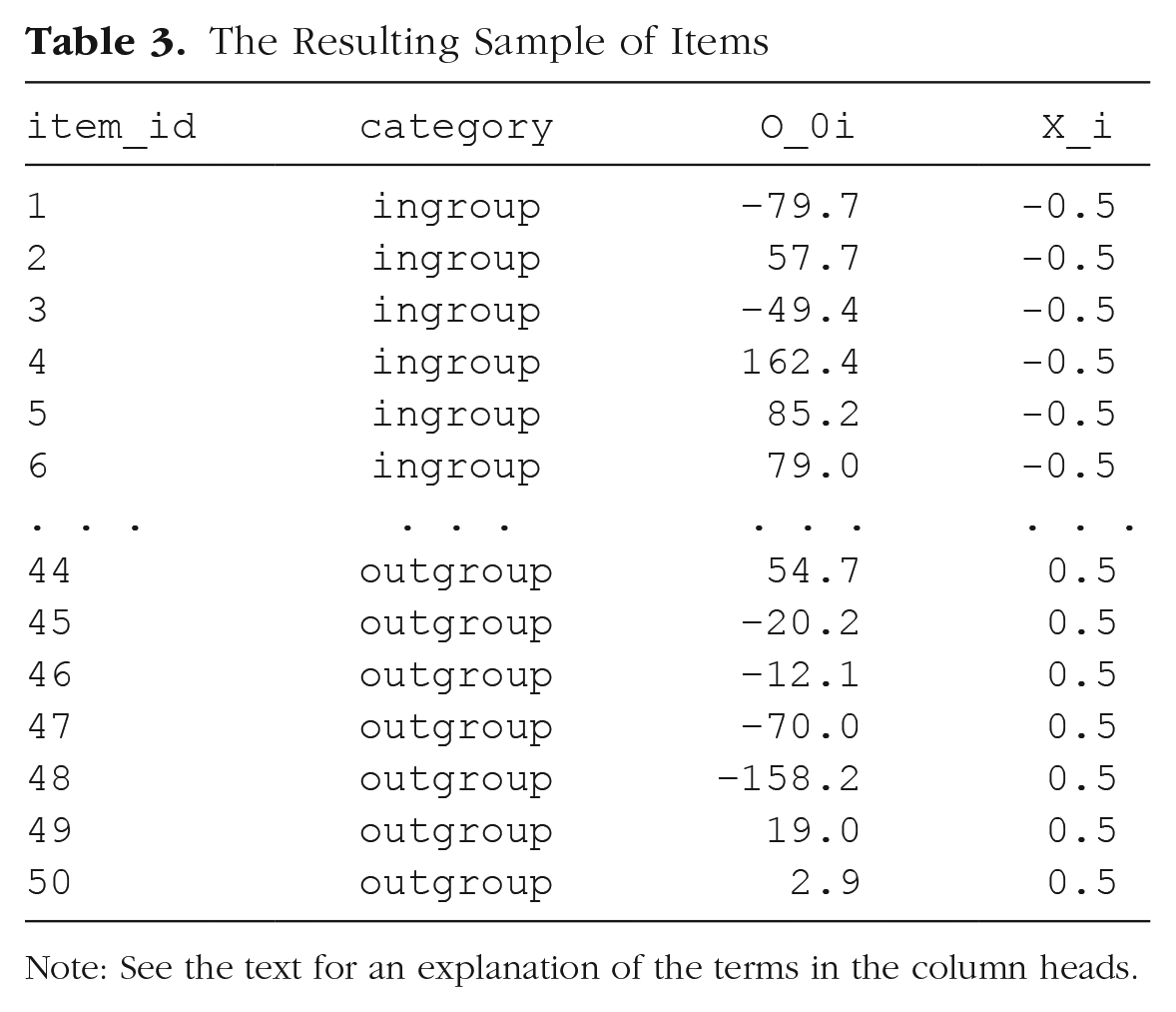
Note: See the text for an explanation of the terms in the column heads.

In R, most regression procedures can handle two-level factors, such as category, as predictor variables. By default, the procedure will create a new numeric predictor that codes one level of the factor as 0 and the other as 1. Why not just use the defaults? The short explanation is that the default of 0, 1 coding is not well suited to the kinds of factorial experimental designs often found in psychology and related fields. For the current example, using the default coding for the X predictor would change the interpretation of β₀: Instead of the grand mean, it would reflect the mean for the group coded as 0. One could change the default, but we feel it is better to be explicit in the code about what values are being used. (See Barr, 2019, for further discussion; see also the R mixed-effects-modeling package afex, by Singmann et al., 2019, which provides better defaults for specifying categorical predictors in ANOVA-style designs.)

Simulate the sampling of subjects

Now we simulate the sampling of individual subjects, which results in a table listing each subject and that subject’s two correlated random effects. This will be slightly more complicated than what we just did, because we cannot simply sample the T_0s values from a univariate distribution using rnorm() independently from the T_1s values. Instead, we must sample < T_0s, T_1s > pairs—one pair for each subject—from a bivariate normal distribution. To do this, we use the mvrnorm() function, a multivariate version of rnorm() from the MASS package that comes preinstalled with R. We need only this one function from MASS, so we can call it directly using the package::function() syntax instead of loading the library (specifically, MASS::mvrnorm() instead of library(MASS)).³ We specify the three parameters describing the distribution of the < T_0s,T_1s > pairs—two variances and a correlation—by entering them into a 2 × 2 variance-covariance matrix using the matrix() function, and then passing this matrix to mvrnorm() using the Sigma argument. This requires converting the standard deviations into variances (by squaring them) and calculating the covariance, which is the product of the correlation and two standard deviations (i.e., ρ × τ₀ × τ₁):



# simulate a sample of subjects


# calculate random intercept / random
 slope covariance
covar <- rho * tau_0 * tau_1


# put values into variance-covariance
 matrix
cov_mx <- matrix(
 c(tau_0^2, covar,
  covar, tau_1^2),
 nrow = 2, byrow = TRUE)


# generate the by-subject random effects
subject_rfx <- MASS::mvrnorm
   (n = n_subj,
   mu = c(T_0s = 0, T_1s = 0),
   Sigma = cov_mx)


# combine with subject IDs
subjects <- data.frame(subj_id =
 seq_len(n_subj),
   subject_rfx)

The resulting table subjects should have the structure shown in Table 4.

Table 4.

The Resulting Sample of Subjects

subj_id	T_0s	T_1s
1	–14.7	11.1
2	–8.4	–36.7
3	87.7	–47.5
4	209.3	62.9
5	–23.6	21.5
6	90.1	56.7
. . .	. . .	. . .
94	99.5	–31.0
95	44.3	69.3
96	12.2	37.1
97	–121.9	42.3
98	–49.9	–41.1
99	–134.5	16.6
100	–30.2	37.5

Note: See the text for an explanation of the terms in the column heads.

An alternative way to sample from a bivariate distribution would be to use the function rnorm_multi() from the faux package (DeBruine, 2020), which generates a table of n simulated values from a multivariate normal distribution by specifying the means (mu) and standard deviations (sd) of each variable, plus the correlations (r), which can be either a single value (applied to all pairs), a correlation matrix, or a vector of the values in the upper right triangle of the correlation matrix:



# simulate a sample of subjects


# sample from a multivariate random
distribution
subjects <- faux::rnorm_multi(
 n = n_subj,
 mu = 0, # means for random effects
  are always 0
 sd = c(tau_0, tau_1), # set SDs
 r = rho, # set correlation, see ?
 faux::rnorm_multi
 varnames = c("T_0s", "T_1s")
)


# add subject IDs
subjects$subj_id <- seq_len(n_subj)

Simulate trials (encounters)

Because all subjects respond to all items, we can set up a table of trials by making a table with every possible combination of the rows in the subject and item tables, using the tidyverse function crossing(). Each trial has random error associated with it, reflecting fluctuations in trial-by-trial performance due to unknown factors; we simulate this by sampling values from a normal distribution with a mean of 0 and standard deviation of sigma:



# cross subject and item IDs; add an
 error term
# nrow(.) is the number of rows in the
 table
trials <- crossing(subjects, items) %>%
 mutate(e_si = rnorm(nrow(.), mean = 0,
  sd = sigma)) %>%
 select(subj_id, item_id, category, X_i,
  everything())

The resulting table should correspond to Table 5.

Table 5.

The Resulting Table of Trials (Encounters)

subj_id	item_id	category	X_i	T_0s	T_1s	O_0i	e_si
1	1	ingroup	–0.50	–14.65	11.13	–79.73	–66.54
1	2	ingroup	–0.50	–14.65	11.13	57.75	–34.74
1	3	ingroup	–0.50	–14.65	11.13	–49.38	–37.49
1	4	ingroup	–0.50	–14.65	11.13	162.35	231.26
1	5	ingroup	–0.50	–14.65	11.13	85.23	–187.64
1	6	ingroup	–0.50	–14.65	11.13	78.98	104.81
. . .	. . .	. . .	. . .	. . .	. . .	. . .	. . .
100	44	outgroup	0.50	–30.15	37.52	54.73	–3.38
100	45	outgroup	0.50	–30.15	37.52	–20.16	18.47
100	46	outgroup	0.50	–30.15	37.52	–12.08	87.92
100	47	outgroup	0.50	–30.15	37.52	–69.99	25.47
100	48	outgroup	0.50	–30.15	37.52	–158.15	91.23
100	49	outgroup	0.50	–30.15	37.52	19.01	78.14
100	50	outgroup	0.50	–30.15	37.52	2.89	–34.31

Note: See the text for an explanation of the terms in the column heads.

Calculate the response values

With this resulting table, in combination with the constants beta_0 and beta_1, we have the full set of values that we need to compute the response variable RT according to the linear model we defined above:

R T_{s i} = β_{0} + T_{0 s} + O_{0 i} + (β_{1} + T_{1 s}) X_{i} + e_{s i} .

Thus, we calculate the response variable RT by adding together

the grand intercept (beta_0),

each subject-specific random intercept (T_0s),

each item-specific random intercept (O_0i),

each sum of the category effect (beta_1) and the subject-specific random slope (T_1s), multiplied by the numeric predictor (X_i), and

each residual error (e_si).

After this, we use dplyr::select() to keep the columns we need:



# calculate the response variable
dat_sim <- trials %>%
 mutate(RT = beta_0 + T_0s + O_0i +
  (beta_1 + T_1s) * X_i + e_si) %>%
 select(subj_id, item_id, category,
  X_i, RT)

Note that the resulting table (Table 6) has the structure that we set as our goal at the start of this exercise, with the additional column X_i, which we will need when we analyze the simulated data later in the Tutorial.

Table 6.

The Final Simulated Data Set

subj_id	item_id	category	X_i	RT
1	1	ingroup	–0.5	609
1	2	ingroup	–0.5	778
1	3	ingroup	–0.5	668
1	4	ingroup	–0.5	1148
1	5	ingroup	–0.5	652
1	6	ingroup	–0.5	939
. . .	. . .	. . .	. . .	. . .
100	44	outgroup	0.5	865
100	45	outgroup	0.5	812
100	46	outgroup	0.5	889
100	47	outgroup	0.5	769
100	48	outgroup	0.5	747
100	49	outgroup	0.5	911
100	50	outgroup	0.5	782

Note: See the text for an explanation of the terms in the column heads.

Data-simulation function

To make it easier to try out different parameters or to generate many data sets for the purpose of power analysis, you can put all of the code above into a custom function. Set up the function to take all of the parameters we set above as arguments. We set the defaults here to the values we used, but you can choose your own defaults. The code below is just all of the code above, condensed a bit. It returns one data set with the parameters specified:



# set up the custom data simulation
 function
my_sim_data <- function(
 n_subj = 100, # number of subjects
 n_ingroup = 25, # number of ingroup
 stimuli
 n_outgroup = 25, # number of outgroup
 stimuli
 beta_0 = 800, # grand mean
 beta_1 = 50, # effect of category
 omega_0 = 80, # by-item random
  intercept sd
 tau_0 = 100, # by-subject random
  intercept sd
 tau_1 = 40, # by-subject random slope sd
 rho = 0.2, # correlation between
  intercept and slope
 sigma = 200) { # residual (standard deviation)
 items <- data.frame(
  item_id = seq_len(n_ingroup +
   n_outgroup),
  category = rep(c("ingroup",
   "outgroup"), c(n_ingroup, n_outgroup)),
  X_i = rep(c(-0.5, 0.5), c(n_ingroup,
   n_outgroup)),
  O_0i = rnorm(n = n_ingroup +
   n_outgroup, mean = 0, sd = omega_0))


 # variance-covariance matrix
 cov_mx <- matrix(
  c(tau_0^2, rho * tau_0 * tau_1,
   rho * tau_0 * tau_1, tau_1^2 ),
  nrow = 2, byrow = TRUE)
 subjects <- data.frame(
  subj_id = seq_len(n_subj),
  MASS::mvrnorm(n = n_subj,
    mu = c(T_0s = 0, T_1s = 0),
    Sigma = cov_mx))
 crossing(subjects, items) %>%
  mutate(e_si = rnorm(nrow(.), mean =
   0, sd = sigma),
   RT = beta_0 + T_0s + O_0i +
    (beta_1 + T_1s) * X_i + e_si) %>%
  select(subj_id, item_id, category,
   X_i, RT)
}

Now you can generate a data set with the default parameters using my_sim_data() or, for example, a data set with 500 subjects and no effect of category using my_sim_data(n_subj = 500, beta_1 = 0).

Analyzing the Simulated Data

Setting up the formula

Now we are ready to analyze our simulated data. The first argument to lmer() is a model formula that defines the structure of the linear model. The formula for our design maps onto how we calculated the variable RT above:



RT ~ 1 + X_i + (1 | item_id) + (1 + X_i
 | subj_id)

The terms in this R formula are as follows:

RT is the response;

1 corresponds to the grand intercept (beta_0);

X_i is the predictor for the in-group/out-group manipulation for item i;

(1 | item_id) specifies an item-specific ran-dom intercept (O_0i);

(1 + X_i | subj_id) specifies a subject-specific random intercept (T_0s) plus the subject-specific random slope of category (T_1s).

The error term (e_si) is automatically included in all models, so it is left implicit. The fixed part of the formula, RT ~ 1 + X_i, establishes the RT_si = β₀ + β₁X_i + e_si part of our linear model. Every model has an intercept (β₀) term and residual term (e_si) by default, so you could alternatively leave the 1 out and just write RT ~ X_i.

The terms in parentheses with the pipe separator (|) define the random-effects structure. For each of these bracketed terms, the left-hand side of the pipe names the effect or effects you wish to allow to vary, and the right-hand side names the variable identifying the levels of the random factor over which they vary (e.g., subjects or items). The first term, (1 | item_id), allows the intercept (1) to vary over the random factor of items (item_id). This is an instruction to estimate the parameter underlying the O_0i values, namely, omega_0. The second term, (1 + X_i | subj_id), allows both the intercept and the effect of category (coded by X_i) to vary over the random factor of subjects (subj_id). It is an instruction to estimate the three parameters that underlie the T_0s and T_1s values, namely, tau_0, tau_1, and rho.

Interpreting the output from lmer()

The other arguments to the lmer() function are the name of the data frame where the values are found (dat_sim). Because we loaded in lmerTest after lme4, the p values are derived using the Satterthwaite approximation, for which the default estimation technique in lmer()—restricted likelihood estimation (REML = TRUE)—is the most appropriate (Luke, 2017). Use the summary() function to view the results:



# fit a linear mixed-effects model to data
mod_sim <- lmer(RT ~ 1 + X_i + (1 | item_
   id) + (1 + X_i | subj_id),
   data = dat_sim)
summary(mod_sim, corr = FALSE)
## Linear mixed model fit by REML. t-tests
use Satterthwaite′s method [
## lmerModLmerTest]
## Formula: RT ~ 1 + X_i + (1 | item_id) + (1 + X_i | subj_id)
## Data: dat_sim
##
## REML criterion at convergence: 67740.7
##
## Scaled residuals:
##   Min   1Q   Median   3Q   Max
## -3.7370 -0.6732  0.0075 0.6708 3.5524
##
## Random effects:
## Groups Name Variance Std.Dev. Corr
## subj_id (Intercept) 8416 91.74
##        X_i   3298  57.43 0.12
## item_id (Intercept) 4072 63.81
## Residual       41283 203.18
## Number of obs: 5000, groups: subj_id, 100; item_id, 50
##
## Fixed effects:
##     Estimate Std. Error df   t value Pr(>|t|)
## (Intercept) 807.72 13.19 119.05 61.258 <2e-16***
##  X_i    39.47  19.79  56.30  1.994  0.051.
## ---
## Signif. codes: 0 ′***′ 0.001 ′**′ 0.01 ′*′
  0.05 ′.′ 0.1 ′ ′ 1

Let us break down the output step-by-step and try to find estimates of the seven parameters we used to generate the data: beta_0, beta_1, tau_0, tau_1, rho, omega_0, and sigma. If you analyze existing data with a mixed-effects model, you can use these estimates to help you set reasonable values for random effects in your own simulations.

After providing general information about the model fit, the output is divided into a Random effects section and a Fixed effects section. The Fixed effects section should be familiar from other types of linear models:



## Fixed effects:
##      Estimate Std. Error df t value Pr(>|t|)
## (Intercept)807.72 13.19 119.05 61.258 <2e-16***
## X_i     39.47 19.79 56.30 1.994 0.051.

The Estimate column gives us parameter estimates for the fixed effects in the model, that is, β₀ and β₁, which are estimated at about 807.72 and 39.47. The next columns give us the standard errors, estimated degrees of freedom (using the Satterthwaite approach), t value, and, finally, p value.

The Random effects section is specific to mixed-effects models, and will be less familiar:



## Random effects:
## Groups  Name    Variance Std.Dev. Corr
## subj_id (Intercept)  8416  91.74
## X_i            3298  57.43 0.12
## item_id (Intercept)  4072  63.81
## Residual         41283 203.18

These are the estimates for the variance components in the model. Note that there are no p values associated with these effects. If you wish to determine whether a random effect is significant, you need to run the model with and without the random-effect term and compare the log likelihoods of the models. But usually the random-effects parameters are not the target of statistical tests because they reflect the existence of individual variation, which can be trivially assumed to exist for any manipulation that has a nonzero effect.

To avoid confusion, it is best to think of the information in the Random effects section as coming from three separate tables divided up by the values in the Groups column. The first subtable, where the value of Groups is subj_id, gives the estimates for the random-effects parameters defining the by-subject random effects:



## Groups  Name    Variance  Std.Dev. Corr
## subj_id (Intercept) 8416    91.74
## X_i           3298    57.43  0.12

We have estimates for the variance of the intercept and slope (X_i) in the Variance column. These estimates are just the squares of the standard deviations in the Std.Dev. column. We obtain estimates for tau_0 and tau_1 of 91.74 and 57.43, respectively. The Corr. column gives us the estimated correlation between the by-subject random intercepts and slopes, estimated here as .12.

The second subtable gives us the by-item random-effects parameter estimates, of which there is only one, 63.81, corresponding to omega_0. Again, the Variance column is just this value squared:



## Groups  Name    Variance Std.Dev. Corr
## item_id (Intercept) 4072   63.81

The last subtable gives us the estimate of the residual term, 203.18:



## Groups  Name Variance Std.Dev. Corr
## Residual     41283  203.18

We have found all seven parameter estimates in the output. The estimated values are reasonably close to the original parameter values that we specified (Table 7).

Table 7.

The Simulation Parameters Compared to the Model Estimations

Variable	Explanation	Simulated value	Estimate from model
beta_0	Intercept; grand-mean reaction time	800.0	807.72
beta_1	Slope; mean effect of the in-group/out-group manipulation	50.0	39.47
tau_0	Standard deviation of the by-subject random intercepts	100.0	91.74
tau_1	Standard deviation of the by-subject random slopes	40.0	57.43
rho	Correlation between the by-subject random intercepts and slopes	0.2	0.12
omega_0	Standard deviation of the by-item random intercepts	80.0	63.81
sigma	Standard deviation of the residuals	200.0	203.18

You can also use broom.mixed::tidy() to output fixed and/or random effects in a tidy table (Table 8):

Table 8.

The Output of the Tidy Function From broom.mixed

effect	group	term	sim	estimate	std.error	statistic	df	p.value
fixed	NA	(Intercept)	800.0	807.72	13.2	61.3	119.1	0.000
fixed	NA	X_i	50.0	39.47	19.8	2.0	56.3	0.051
ran_pars	subj_id	sd__(Intercept)	100.0	91.74	NA	NA	NA	NA
ran_pars	subj_id	cor__(Intercept).X_i	0.2	0.12	NA	NA	NA	NA
ran_pars	subj_id	sd__X_i	40.0	57.43	NA	NA	NA	NA
ran_pars	item_id	sd__(Intercept)	80.0	63.81	NA	NA	NA	NA
ran_pars	Residual	sd__Observation	200.0	203.18	NA	NA	NA	NA

Note: See the text for an explanation of the terms in this table. NA = not applicable.



# get a tidy table of results
broom.mixed::tidy(mod_sim) %>%
 mutate(sim = c(beta_0, beta_1, tau_0,
  rho, tau_1, omega_0, sigma)) %>%
 select(1:3, 9, 4:8)

This is especially useful when you need to combine the output from hundreds of simulations to calculate power. The effect column specifies whether a row is a fixed-effect (fixed) or a random-effect (ran_pars) parameter. The group column specifies which random factor each random-effect parameter belongs to (or Residual for the residual term). The term column refers to the predictor term for fixed effects and also the parameter for random effects; for example, “sd__X_i” refers to the standard deviation of the random slope for X_i, and “cor__(Intercept).X_i” refers to rho, the correlation between the random intercept and slope for X_i. We added the sim column to the standard output of broom.mixed::tidy() so you can compare the simulated parameters we set above with the estimated parameters from this simulated data set, which are in the estimate column. The last four columns give the standard error, t statistic, estimated degrees of freedom, and p value for the fixed effects.

Setting parameters

Now that you see where each parameter we used to generate the data appears in the analysis output, you can use the analysis of pilot data to get estimates for these parameters for further simulation. For example, if you have pilot data from 10 participants on this task, you can analyze their data using the same code as above and estimate values for beta_0, beta_1, tau_0, tau_1, rho, omega_0, and sigma for use in a power calculation or a sensitivity analysis (see Appendix 1C at our OSF project page). If you lack any pilot data to work with, you can start with the general rule of thumb and set the residual variance to about twice the size of the by-subject or by-item variance components (see Barr et al., 2012, for results from an informal convenience sample).

Calculate Power

Data simulation is a particularly flexible approach for estimating power when planning a study. The basic idea of a power simulation is to choose parameter values with which to generate a large number of data sets, fit a model to each data set, and then calculate the proportion of models that reject the null hypothesis. This proportion is an estimate of power for those particular parameter values. To estimate power accurately using Monte Carlo simulation, you need to generate and analyze a large number (typically, hundreds or thousands) of data sets.

In a Monte Carlo power simulation, it is useful to create a function that performs all the steps corresponding to a single Monte Carlo “run” of the simulation: generate a data set, analyze the data, and return the estimates. The function single_run() below performs all these actions:



# simulate, analyze, and return a
table of parameter estimates
single_run <- function(. . .) {
 # . . . is a shortcut that forwards
any arguments to
 # my_sim_data(), the function created
above
 dat_sim <- my_sim_data(. . .)
 mod_sim <- lmer(RT ~ X_i + (1 | item_
  id) + (1 + X_i | subj_id),
    dat_sim)
 broom.mixed::tidy(mod_sim)
}
# run one model with default parameters
single_run()

You can also change parameters. For example, what would happen if you increase the number of items to 50 in each group and decrease the effect of category to 20 ms, as in the following code?



# run one model with new parameters
single_run(n_ingroup = 50, n_outgroup =
50, beta_1 = 20)

Example results of a single run with these parameters are shown in Table 9.

Table 9.

The Output of single_run() With 50 Items per Group and a Category Effect of 20 ms

effect	group	term	estimate	std.error	statistic	df	p.value
fixed	NA	(Intercept)	832.38	12.6	66.1	174.0	0.000
fixed	NA	X_i	24.95	16.0	1.6	114.9	0.121
ran_pars	item_id	sd__(Intercept)	73.66	NA	NA	NA	NA
ran_pars	subj_id	sd__(Intercept)	100.27	NA	NA	NA	NA
ran_pars	subj_id	cor__(Intercept).X_i	0.00	NA	NA	NA	NA
ran_pars	subj_id	sd__X_i	47.57	NA	NA	NA	NA
ran_pars	Residual	sd__Observation	199.15	NA	NA	NA	NA

Note: See the text for an explanation of the terms in this table. NA = not applicable.

You can use the purrr::map_df function to run the simulation repeatedly and save the results to a data table. This will take a while, so test the code first using just a few runs (n_runs) to debug it and check the output. Once you are satisfied that it is working properly, we suggest that you use at least a thousand runs to obtain stable estimates. It will save you a lot of time if you save the full results to disk:



# run simulations and save to a file
n_runs <- 100 # use at least 1000 to
 get stable estimates
sims <- purrr::map_df(1:n_runs, ~
 single_run())
write_csv(sims, "sims.csv")

This way, you do not have to rerun this subroutine each time you execute your script; you can just comment out this code and load the saved data when you use this script in the future.

Note that some runs may throw warnings about nonconvergence or messages about boundary (singular) fit. Messages about the singular fit can usually be ignored (see the lme4 help documentation ?isSingular for information). Nonconvergence will be relatively rare with simulated data provided the sample is not unreasonably small relative to the number of estimated parameters; as long as there are not too many of these nonconvergence warnings relative to the number of runs, you can probably ignore them because they will not affect the overall estimates. Alternatively, you can rewrite your function to trap the warning (see Appendix 1C at our OSF project page; for more information on trapping errors and warnings, see the chapter “Exceptions and Debugging” in Wickham’s, 2019, Advanced R textbook).

Once our simulations are complete, let us read the data back in and have a look at the estimates for our fixed effects:



# read saved simulation data
sims <- read_csv("sims.csv", col_types =
cols(
 # makes sure plots display in this order
 group = col_factor(ordered = TRUE),
 term = col_factor(ordered = TRUE)
 ))
sims %>%
 filter(effect == "fixed") %>%
 select(term, estimate, p.value)
## # A tibble: 200 x 3
## term estimate p.value
## <ord> <dbl> <dbl>
## 1 (Intercept) 813. 2.93e-86
## 2 X_i 83.4 3.53e- 4
## 3 (Intercept) 799. 1.25e-82
## 4 X_i 57.9 1.58e- 2
## 5 (Intercept) 782. 6.17e-88
## 6 X_i 63.9 4.54e- 3
## 7 (Intercept) 812. 1.97e-83
## 8 X_i 45.7 4.78e- 2
## 9 (Intercept) 824. 8.69e-77
## 10 X_i 1.78 9.45e- 1
## # . . . with 190 more rows

Each row in the table is an estimate of a fixed-effects parameter and associated p value from a single run of the Monte Carlo simulation ((Intercept) = β₀ and X_i = β₁). We need to calculate the proportion of runs with significant results. To start, we compute p.value < alpha, where alpha is the false-positive rate (e.g., .05):



# calculate mean estimates and power for
 specified alpha
alpha <- 0.05
sims %>%
 filter(effect == "fixed") %>%
 group_by(term) %>%
 summarize(
  mean_estimate = mean(estimate),
  mean_se = mean(std.error),
  power = mean(p.value < alpha),
  .groups = "drop"
 )

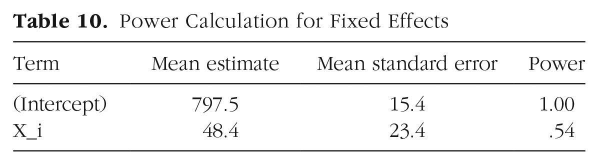
This will yield a logical vector of TRUE whenever the effect was significant and FALSE when it was nonsignificant. Because TRUE is represented internally as a 1 and FALSE as a 0, you can take the mean of this logical vector, and it will yield the proportion of runs with significant results.

The results of our power analysis appear in Table 10. The attained power of .54 in the second row is the estimated probability of finding a significant effect of category (as represented by X_i) given our starting parameters. In other words, it is the probability of rejecting the null hypothesis (H₀) for β₁, which is the coefficient associated with X_i in the model (H₀: β₁ = 0). If we wanted to see how power changes with different parameter settings, we would need to rerun the simulations with different values passed to single_run().

Table 10.

Power Calculation for Fixed Effects

Term	Mean estimate	Mean standard error	Power
(Intercept)	797.5	15.4	1.00
X_i	48.4	23.4	.54

Conclusion

Mixed-effects modeling is a powerful technique for analyzing data from complex designs. The technique is close to ideal for analyzing data with crossed random factors of subjects and stimuli: It gracefully and simultaneously accounts for subject and item variance within a single analysis and outperforms traditional techniques in terms of Type I error and power (Barr et al., 2013). However, this additional power comes at the price of technical complexity. Through this article, we have attempted to make mixed-effects models more approachable using data simulation.

We have considered only a simple, one-factor design. However, the general principles are the same for higher-order designs. For instance, consider a 2 × 2 design, with factors A and B both within subjects, but A within items and B between items. For such a design, you would have four instead of two by-subject random effects: the intercept, main effect of A, main effect of B, and AB interaction. You would also need to specify correlations between each pair of these effects. You would also have two by-item random effects: one for the intercept and one for A. Our materials at OSF include such an extension of the example in this article with category as a within-subjects and between-items factor and expression added as a within-subjects and within-items factor (see Appendix 2: Extended Examples, at https://osf.io/ut3rx/). For further guidance and discussion on how to specify the random-effects structure in complex designs, see Barr (2013).

Here we have considered only a design with a normally distributed response variable. However, generalized linear mixed-effect models allow for response variables with different distributions, such as binomial distributions. Our materials at OSF illustrate the differences in simulation required for the study design discussed in this article if a binomial accuracy score (correct/incorrect) is the response variable (see Appendix 3a: Binomial Example, at https://osf.io/vxnm8/, and Appendix 3b: Extended Binomial Example, at https://osf.io/mt5nw/).

We also have not said much in this Tutorial about estimation issues, such as what to do when the fitting procedure fails to converge. Further guidance on this point can be found in Barr et al. (2013), as well as in the help materials in the lme4 package (?lme4::convergence). We have also assumed that the random-effects specification for the lmer() function should be based on the study design. However, we note that other researchers have argued in favor of data-driven approaches for random-effects specification (Matuschek et al., 2017). In this Tutorial, we have introduced the main concepts needed to get started with mixed-effects models. Through data simulation of your own study designs, you can develop your understanding and perform power calculations to guide your sample-size plans.

Footnotes

Transparency

Action Editor: Mijke Rhemtulla

Editor: Daniel J. Simons

Author Contributions

D. J. Barr drafted the substantive explanation, and L. M. DeBruine drafted the tutorial example. Both authors revised the draft of the manuscript and approved the final submitted version. L. M. DeBruine created the app ().

ORCID iDs

Lisa DeBruine

Dale J. Barr

Notes

References

Aust

Barth

(2018). papaja: Create APA manuscripts with R Markdown (Version 0.1.0.9997) [Computer software]. GitHub. https://github.com/crsh/papaja

Baayen

R. H.

Davidson

D. J.

Bates

D. M.

(2008). Mixed-effects modeling with crossed random effects for subjects and items. Journal of Memory and Language, 59(4), 390–412.

Barr

(2019, April 2). Coding categorical predictor variables in factorial designs. talklab. https://talklab.psy.gla.ac.uk/tvw/catpred/

Barr

D. J.

(2013). Random effects structure for testing interactions in linear mixed-effects models. Frontiers in Psychology, 4, Article 328. https://doi.org/10.3389/fpsyg.2013.00328

Barr

D. J.

(2018). Generalizing over encounters: Statistical and theoretical considerations. In Rueschemeyer

S.-A.

Gaskell

M. G.

(Eds.), Oxford handbook of psycholinguistics (pp. 917–929). Oxford University Press.

Barr

D. J.

Levy

Scheepers

Tily

H. J.

(2012). Random effects in real datasets. talklab. https://talklab.psy.gla.ac.uk/simgen/realdata.html

Barr

D. J.

Levy

Scheepers

Tily

H. J.

(2013). Random effects structure for confirmatory hypothesis testing: Keep it maximal. Journal of Memory and Language, 68(3), 255–278.

Bates

Mächler

Bolker

Walker

(2015). Fitting linear mixed-effects models using lme4. Journal of Statistical Software, 67(1). https://doi.org/10.18637/jss.v067.i01

Bedny

Aguirre

G. K.

Thompson-Schill

S. L.

(2007). Item analysis in functional magnetic resonance imaging. NeuroImage, 35(3), 1093–1102.

10.

Bolker

Robinson

(2019). broom.mixed: Tidying methods for mixed models (Version 0.2.5) [Computer software]. Comprehensive R Archive Network. https://CRAN.R-project.org/package=broom.mixed

11.

Clark

H. H.

(1973). The language-as-fixed-effect fallacy: A critique of language statistics in psychological research. Journal of Verbal Learning and Verbal Behavior, 12(4), 335–359.

12.

Coleman

E. B.

(1964). Generalizing to a language population. Psychological Reports, 14(1), 219–226.

13.

DeBruine

(2020). faux: Simulation for factorial designs (Version 0.0.1.5) [Computer software]. Zenodo. https://doi.org/10.5281/zenodo.2669586

14.

Forster

Dickinson

(1976). More on the language-as-fixed-effect fallacy: Monte Carlo estimates of error rates for F₁,F₂,F′, and min F′. Journal of Verbal Learning and Verbal Behavior, 15(2), 135–142.

15.

Judd

C. M.

Westfall

Kenny

D. A.

(2012). Treating stimuli as a random factor in social psychology: A new and comprehensive solution to a pervasive but largely ignored problem. Journal of Personality and Social Psychology, 103(1), 54–69.

16.

Kuznetsova

Brockhoff

P. B.

Christensen

R. H. B.

(2017). lmerTest package: Tests in linear mixed effects models. Journal of Statistical Software, 82(13). https://doi.org/10.18637/jss.v082.i13

17.

Locker

Hoffman

Bovaird

J. A.

(2007). On the use of multilevel modeling as an alternative to items analysis in psycholinguistic research. Behavior Research Methods, 39(4), 723–730.

18.

Luke

S. G.

(2017). Evaluating significance in linear mixed-effects models in R. Behavior Research Methods, 49(4), 1494–1502.

19.

Matuschek

Kliegl

Vasishth

Baayen

Bates

(2017). Balancing Type I error and power in linear mixed models. Journal of Memory and Language, 94, 305–315.

20.

R Core Team. (2018). R: A language and environment for statistical computing (Version 4.0.1) [Computer software]. R Foundation for Statistical Computing. https://www.Rproject.org/

21.

Singmann

Bolker

Westfall

Aust

(2019). afex: Analysis of factorial experiments (Version 0.27.2) [Computer software]. Comprehensive R Archive Network. https://CRAN.R-project.org/package=afex

22.

Westfall

Kenny

D. A.

Judd

C. M.

(2014). Statistical power and optimal design in experiments in which samples of participants respond to samples of stimuli. Journal of Experimental Psychology: General, 143(5), 2020–2045.

23.

Westfall

Nichols

T. E.

Yarkoni

(2017). Fixing the stimulus-as-fixed-effect fallacy in task fMRI. Wellcome Open Research, 1, Article 23. https://doi.org/10.12688/wellcomeopenres.10298.2

24.

Wickham

(2017). tidyverse: Easily install and load the ‘tidyverse (Version 1.2.1) [Computer software]. Comprehensive R Archive Network. https://CRAN.R-project.org/package=tidyverse

25.

Wickham

(2019). Advanced R. CRC Press. http://adv-r.had.co.nz/

26.

Yarkoni

(2020). The generalizability crisis. Behavioral and Brain Sciences. Advance online publication. https://doi.org/10.1017/S0140525X20001685

Understanding Mixed-Effects Models Through Data Simulation

Abstract

Keywords

Generalizing to a Population of Encounters

Disclosures

Simulating Data With Crossed Random Factors

Required software

Establishing the data-generating parameters

Specify the data structure

Specify the fixed-effects parameters

Specify the random-effects parameters

Simulating the sampling process

Simulate the sampling of stimulus items

Simulate the sampling of subjects

Simulate trials (encounters)

Calculate the response values

Data-simulation function

Analyzing the Simulated Data

Setting up the formula

Interpreting the output from lmer()

Setting parameters

Calculate Power

Conclusion

Footnotes

Transparency

ORCID iDs

Notes

References