Tutorial: Power Analyses for Interaction Effects in Cross-Sectional Regressions

Abstract

Interaction analyses (also termed “moderation” analyses or “moderated multiple regression”) are a form of linear regression analysis designed to test whether the association between two variables changes when conditioned on a third variable. It can be challenging to perform a power analysis for interactions with existing software, particularly when variables are correlated and continuous. Moreover, although power is affected by main effects, their correlation, and variable reliability, it can be unclear how to incorporate these effects into a power analysis. The R package InteractionPoweR and associated Shiny apps allow researchers with minimal or no programming experience to perform analytic and simulation-based power analyses for interactions. At minimum, these analyses require the Pearson’s correlation between variables and sample size, and additional parameters, including reliability and the number of discrete levels that a variable takes (e.g., binary or Likert scale), can optionally be specified. In this tutorial, we demonstrate how to perform power analyses using our package and give examples of how power can be affected by main effects, correlations between main effects, reliability, and variable distributions. We also include a brief discussion of how researchers may select an appropriate interaction effect size when performing a power analysis.

Interaction analyses (also termed “moderation” analyses or “moderated multiple regression”) are a form of linear regression analysis designed to test whether the association between two variables changes when conditioned on a third variable, for example, whether the association between a trait and an outcome differs between groups. Interactions and equivalent tests, such as two-way analyses of variance, are widely tested across the psychological and social sciences, yet there is growing concern that they contribute to the low replicability of findings in these fields (Altmejd et al., 2019; Open Science Collaboration, 2015; Vize et al., 2022). In tandem, there is increasing evidence that the effect sizes of interactions in observational designs are quite small (Aguinis et al., 2005; Beck & Jackson, 2020; Sherman & Pashler, 2019; Sommet et al., 2022; Tosh et al., 2021; Vize et al., 2022). In the context of these concerns, power analyses can be a critically useful tool for ensuring the robustness and accuracy of conclusions resulting from tests of interactions.

A power analysis is a simulation or calculation of how likely it is that a statistical test will detect a significant result, assuming a true nonzero effect in the population. Power analyses at minimum require the user to specify an effect size, sample size, and alpha (i.e., the p-value threshold that determines whether a result is significant). If the power analysis is run as a simulation, it is simply the percentage of simulations in which a significant result is found. Power analyses have many uses, including (a) determining the needed sample size to test an effect, (b) determining whether an existing data set can detect an effect of interest, and (c) aiding in the interpretation of findings (i.e., a sensitivity analysis; Baranger et al., 2020). It can be quite challenging to correctly perform a power analysis for an interaction, particularly because many of the most widely used tools were designed with experimental manipulations in mind (i.e., factorial designs) and are difficult to apply when planning an observational study, especially with continuous data. For example, they may assume that variables are uncorrelated or require effect sizes (e.g., $f^2$ ) that are computed by first solving a system of simultaneous linear equations (see the Supplemental Material available online), which can be a significant barrier. Moreover, it is well known that variable reliability affects power, although it can frequently be unclear how to incorporate it into a power analysis.

In this article, we introduce the InteractionPoweR R package and accompanying Shiny apps, which contain functions for power analyses of interactions with cross-sectional data. This software is free to use, and the Shiny apps do not require any programming experience. Compared with G*Power and the Superpower and pwr2ppl R packages (Aberson, 2019; Faul et al., 2007; Lakens & Caldwell, 2021), InteractionPoweR requires only the standardized cross-sectional effect size (i.e., Pearson’s correlation coefficient), which makes it easy to obtain effect sizes from the published literature to inform a power analysis. InteractionPoweR is also unique in several important ways. First, it incorporates the correlation between the interacting variables, resulting in more accurate power estimates and frequently greater power than estimates that assume variable independence (Shieh, 2010). Second, it incorporates variable reliability, which can dramatically affect power (Brunner & Austin, 2009). Third, variables can be noncontinuous (i.e., binary or ordinal). In this tutorial, we demonstrate how to use InteractionPoweR to run a power analysis for interactions and highlight how power is dependent on main effects, variable correlations, reliability, and variable distributions.

A Brief Introduction to Interactions

Written symbolically, interaction analyses take the form

$$Y=B_0+B_1{X}_1+B_2{X}_2+B_3{X}_1{X}_2+\mathrm{\epsilon },$$

where Y is the dependent variable, $X_1$ and $X_2$ are the independent variables, $X_1{X}_2$ is the interaction term (i.e., $X_1\times X_2$ ), B refers to standardized effect sizes ( $B_0$ is the intercept), and $\epsilon$ is the error. Thus, the term of interest is $B_3$ , the effect size of the interaction. A significant interaction (e.g., p < .05) will indicate that the association between each of the independent variables and the dependent variable changes when conditioned on the other (i.e., the association between $X_1$ and $Y$ varies when conditioned on $X_2$ and vice versa), assuming the model is valid (e.g., no omitted variables); see the discussion in the next section about the importance of this assumption. In this tutorial, we refer to $X_2$ as the “moderator” and $X_1$ as the “variable of interest,” but it is important to note that these two are interchangeable (Finsaas & Goldstein, 2021), and the interaction analysis itself provides no evidence for causal effects (Rohrer & Arslan, 2021).

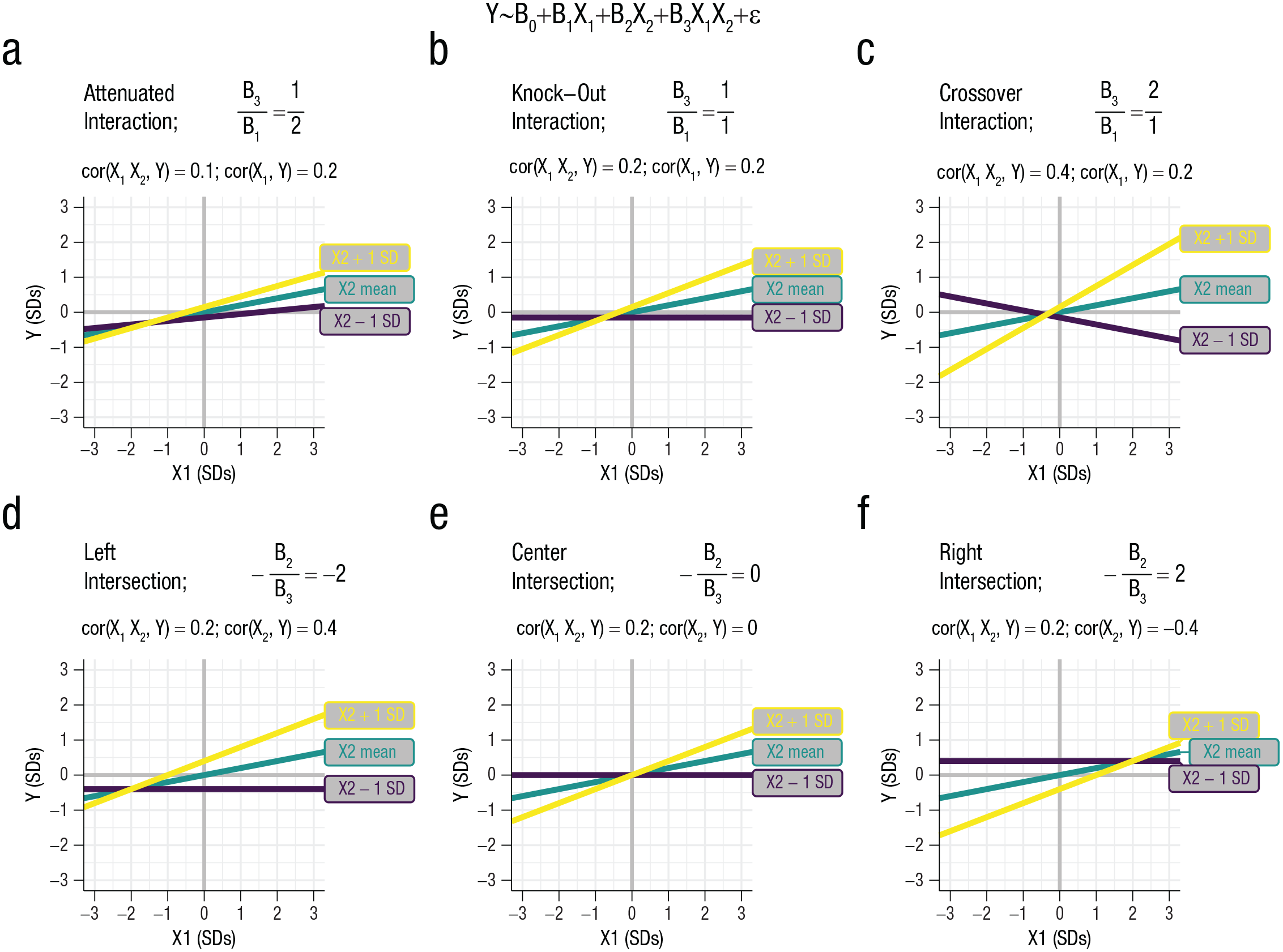
One challenging aspect of performing a power analysis for an interaction is selecting an appropriate value for the magnitude of the interaction effect—the correlation between $X_1{X}_2$ and Y. A common practice is to interpret interaction effects in light of the simple slopes (i.e., the association between $X_1$ and Y at different values of X₂; Aiken & West, 1991; see also Finsaas & Goldstein, 2021) and where the simple slopes intersect. Moreover, theories may hypothesize that the simple slopes will take a particular form or intersect at particular values of the main effect (e.g., the differential susceptibility and diathesis-stress hypotheses; Belsky & Pluess, 2009; Widaman et al., 2012). However, this focus on simple slopes can make it challenging to select an appropriate effect size for a power analysis because it can be unclear what a specific correlation means in terms of the simple slopes (e.g., is r = .1 a small or large effect?). A key insight is that the shape and intersection of the simple slopes is a result of the magnitude of the interaction effect ( $B_3$ ) relative to the magnitude of the main effects ( $B_1$ and $B_2$ ; note that, as above, $B_1$ is referred to here as the “main effect” and $B_2$ as the “moderator,” although they are interchangeable; Fig. 1). The shape of an interaction is governed by the ratio of the interaction effect ( $B_3$ ) to the main effect $B_1$ . If the ratio of these effects is less than 1, then the effect is an “attenuated” effect, in which both simple slopes are in the same direction (Fig. 1a). If these effects are the same size (a ratio of 1), then the interaction is a “knock-out” effect, in which one of the simple slopes is a flat line (a slope of 0; Fig. 1b). If the ratio is larger than 1, then the effect is a “crossover” effect, in which one simple slope is positive and the other is negative (Fig. 1c). Where the simple slopes intersect is governed by the ratio of the moderator effect $B_2$ to the interaction effect $B_3.$ If both effects are in the same direction (both positive or both negative), then the simple slopes will intersect at negative values of $X_1$ (Fig. 1d). If $B_2$ and $B_3$ are in opposing directions (one negative and one positive), then the simple slopes will intersect at positive values of $X_1$ (Fig. 1f). Note as well that if one begins with known main effects and a hypothesized interaction shape, the corresponding interaction effect size can be easily derived.

Fig. 1.

The shape of an interaction. Examples of interactions with different shapes are shown. Simple slopes are plotted at −1 SD, the mean, and +1 SD. All variables are continuous and normally distributed. (a–c) The interaction, the correlation between $X_1{X}_2$ and Y, is varied (rs = .1, .2, .4). The correlation between $X_1$ and Y is r = .2, the correlation between $X_2$ and Y is r = .15, the correlation between $X_1$ and $X_2$ is r = .0. (a) An attenuated effect (also termed “partially attenuated”); the interaction effect is smaller than the main effect, and all simple-slope effects are in the same direction. (b) A knock-out or “no-way” interaction (also termed “fully attenuated”); the interaction effect and main effect are the same size. One of the simple slopes is 0—there is no effect of $X_1$ at that level of $X_2$ . (c) A crossover or “butterfly” interaction. The interaction effect is larger than the main effect, and the simple slopes are in opposite directions. (d–f) The correlation between $X_2$ and Y is varied (rs = .4, 0, –.4). The correlation between $X_1$ and Y is r = .2, the correlation between $X_1{X}_2$ and Y is r = .2, and the correlation between $X_1$ and $X_2$ is r = .0. Depending on the ratio of the moderator and interaction effect, the simple slopes can intersect at (d) negative values of X₁, (e) zero, or (f) positive values of X₁. Note that these figures are illustrations of common interactions, but power to detect each interaction is not a function of any general pattern (e.g., crossover does not inherently require more power than knock-out).

Tools for interaction power analyses

InteractionPoweR includes two functions for computing power: power_interaction() and power_interaction_r2() (Table 1). The first function, power_interaction(), simulates multiple data sets with the correlations and sample size specified by the user and runs a regression in each data set. Power is computed as the percentage of simulated data sets in which the interaction is significant. The second function, power_interaction_r2(), determines power analytically by solving for Cohen’s $f^2$ and computing the noncentrality parameter (λ) of the F distribution, from which power is a direct result (Cohen, 1988; Maxwell, 2000). Further details on the methodology underlying these functions are given in the Supplemental Material. Both functions are also accessible via online web applications: https://mfinsaas.shinyapps.io/InteractionPoweR/ for power by simulation and https://david-baranger.shinyapps.io/InteractionPoweR_analytic/ for analytic power. Each approach has its own advantages. Analytic power is much faster to compute than simulation-based power. Simulation-based power, on the other hand, (a) allows for variables to be binary or ordinal and (b) permits users to look beyond simply computing power. For example, users can also examine the range of effect sizes, simple slopes, and interaction shapes observed in a sample that would be consistent with a given population effect size, which can be useful both in planning and interpreting analyses.

Table 1.

Methods for Interaction Power Analyses

Methods for interaction power analyses
R package: https://cran.r-project.org/package=InteractionPoweR
Additional documentation: https://dbaranger.github.io/InteractionPoweR/index.html
Primary power-analysis functions
	Data simulation	Analytic power
Function	power_interaction()	power_interaction_r2()
Web application	https://mfinsaas.shinyapps.io/InteractionPoweR/	https://david-baranger.shinyapps.io/InteractionPoweR_analytic/
Advantages	● Variables can be binary or ordinal ● Examine the distribution of effects in samples consistent with a population effect size	● Fast to compute
Additional functions in the R package
Function	Use
plot_power_curve()	Plots the power curve from a power analysis
power_estimate()	Uses polynomial regression to estimate where the power curve achieves the desired level of power
generate_interaction()	Simulates single data set with the specified interaction
plot_interaction()	Plots the interaction in a single simulated data set
test_interaction()	Runs a regression testing the interaction in a single simulated data set

Note: Functions and web applications for power analyses for interaction analyses provided in the InteractionPoweR package. Further detail on the use of these functions can be found in the package documentation.

We also note an important limitation of the power-analysis functions presented here, which is that they assume that the relatively simple interaction model presented above is a valid model of the data under investigation. Specifically, it is assumed that there are no omitted variables that correlate with or depend on $X_1$ , $X_2$ , and $X_1{X}_2$ . This includes confounding variables (Rohrer et al., 2022) and also extends to nonlinear relationships between $X_1$ and $X_2$ and Y (e.g., it is assumed that $X_1^2$ explains no additional variation in Y after accounting for $X_1$ ; Hainmueller et al., 2019). Another important assumption of these analyses is that the variables under investigation are normally distributed and symmetric in both lower and higher dimensions (e.g., skew = 0). Thus, after mean-centering and under these assumptions, the interaction term $X_1{X}_2$ is largely uncorrelated with $X_1$ and $X_2$ because these correlations are partially a function of the expected value of $X_1$ and $X_2$ , which is now 0 (Olvera Astivia & Kroc, 2019). The extent to which the user’s real-world data violate these assumptions will determine the accuracy and utility of the power analysis. There is no test for omitted variable bias, although methods have been proposed to evaluate its potential impact (Diegert et al., 2022; Wilms et al., 2021). Note as well that the list of potential omitted variables greatly expands if the interaction model includes covariates (Keller, 2014). Researchers can also examine the distribution and correlation of variables in their sample, and we also recommend including individual data points in visualizations of interactions, including both plotting simple slopes and plotting the interaction term against $X_1$ and $X_2$ (Olvera Astivia & Kroc, 2019) to determine whether assumptions are met. These limitations notwithstanding, we believe these functions will be useful tools for researchers even in the case when these assumptions do not all hold because they can be used to gain a deeper understanding of how to interpret interaction models and the relationship between power, effect sizes, and variable correlations in interaction models.

A simple example

Take an example of a hypothetical interaction. Say that you have a known interaction—that the strength of the association between neuroticism (your outcome) and depressive symptoms (the main effect) varies as a function of stressful life events (SLEs; the moderator; Bondy et al., 2021). You have a new sample and would like to know your power to detect this interaction. To do so, you need the correlation between neuroticism and depressive symptoms ( $X_1$ and Y ; r = .51), the correlation between SLEs and depressive symptoms ( $X_2$ and Y ; r = .22), the correlation between neuroticism and SLEs ( $X_1$ and $X_2$ ; r = .09), and your sample size (say, N = 940). Finally, you need a hypothesized interaction effect size—how much the association between neuroticism and depressive symptoms changes for every 1 SD change in SLEs—the correlation between the Neuroticism × SLEs interaction term and depressive symptoms. In the present example, this can be drawn from the prior literature (r = .09). See Figure 2a for a schematic of this interaction and Figure 2b for an example of a single data set drawn from these population-level parameters.

Fig. 2.

Example power analysis. (a) Depiction of the population-level effect. X₂ is the moderator. X₂ groups depict the simple slopes at mean ±1 SD. (b) Depiction of the same effect in a sample of 940 participants. Generated using the generate_interaction() function and plotted using the plot_interaction() function. (c) An analytic power analysis for the hypothesized effect at N = 940. The code for this analysis is InteractionPoweR::power_interaction_r2(N = 940,r.x1.y = 0.51,r.x2.y = 0.22,r.x1.x2 = 0.09,r.x1x2.y = 0.09,alpha = 0.05). There is 90% power (0.9). ¹ (d) Distribution of the “shape” parameter ( $B_3$ / $B_1$ ) from 10,000 simulations generated by the power_interaction() function. Color indicates the range of the 95% confidence interval. The x-axis is the log-transformed ratio of the interaction term (B₃) and main effect of X₁ (B₁).

The standardized effect sizes described in the equation above can be calculated from these correlations via path-tracing (see the Supplemental Material). Note that all variables are standardized in these calculations such that M = 0 and SD = 1. Because the variables are mean-centered, the intercept is 0, and the correlation between $X_1{X}_2$ and $X_1$ and the correlation between $X_1{X}_2$ and $X_2$ is r = 0 as long as the variables are normally distributed and symmetric in both lower and higher dimensions (Olvera Astivia & Kroc, 2019). Example code using the InteractionPoweR function for analytic power power_interaction_r2 and the result of this analysis is given in Figure 2c. You see that your analysis would have 90% power to detect your effect with an alpha of .05 (i.e., you would detect a significant effect 90% of the time). Figure 2d shows the distribution of the interaction’s shape ( $B_3$ / $B_1$ ) across 10,000 simulations (generated via the interaction_power() function; see code in the Supplemental Material). Although the hypothesized shape is approximately 1:5 (an attenuated effect—the interaction effect is one-fifth the size of the main effect), shapes ranging from 1:3 to 1:14 are likely to be observed in a new sample with 90% power (95% of simulated interactions fall within this range).

Planning a Study

Finding the necessary sample size

Power analyses are frequently used when planning a study. Taking the example in the prior section, say that you are planning your replication study but wish to account for possible effects of publication bias and measurement error (for an extended discussion of this complex issue, see Anderson & Kelley, 2022). In your case, you decide that the effect size reported in the original study may be inflated and decide to plan on powering your analysis to detect an interaction effect size that is half of what was reported in the original study—the correlation between $X_1{X}_2$ and Y of r = .045 instead of r = .09 (Fig. 3a). How many participants would you need in your study to have 90% power to detect that effect? As opposed to entering a single value for the sample size, you can enter a range of values, say from N = 500 to N = 6,000, and examine power at all of them (Fig. 3c). The function plot_power_curve() plots the power curve (Fig. 3b), visual inspection of which indicates that you would need approximately a sample size of 3,750 to detect your hypothesized interaction with 90% power.

Fig. 3.

Finding the necessary sample size. (a) Depiction of the population-level effect. X₂ is the moderator. X₂ groups depict the simple slopes at mean ±1 SD. (b) Power curve for the effect of interest, made using the plot_power_curve function. N = 3,750 achieves 90% power. (c) Code for the analytic power analysis used to generate Fig. 3b. Sample size (N) ranges from 500 to 6,000 in increments of 250. The code for this analysis is: InteractionPoweR::power_interaction_r2(N = seq(500,6000,250),r.x1.y = 0.51,r.x2.y = 0.22,r.x1.x2 = 0.09,r.x1x2.y = 0.045,alpha = 0.05). ²

Finding the minimum detectable effect size—also known as the sensitivity power

Note that any of the parameters can be varied in the simulation. For example, if you are planning an analysis in a data set that already exists or evaluating an analysis that has already been conducted, you can instead vary the correlation between $X_1{X}_2$ and Y, which allows you to determine the smallest detectable effect size. We remind the reader that one should not draw these effects directly from an analysis that has already been performed (Gelman & Carlin, 2014; Zhang et al., 2019) unless there is high confidence that the observed sample effect is a reasonably precise estimate of the population-level effect. Power is a function of population-level effects, whereas estimates from individual samples are likely to be biased, particularly because publication bias and selection on significant effects lead to overestimates of effect sizes (Kühberger et al., 2014). Thus, a sensitivity analysis using observed sample effects risks being circular because it confounds sample and population-level effects and will inevitably yield a high “power” estimate, merely reflecting that the observed sample-level effect used in the analysis was significant.

Returning to your original sample size of 940, say that you have evaluated the costs and benefits and decided that you need only 80% power, not 90% power. What is then the minimum detectable interaction effect size? You can test a range of values for the correlation between $X_1{X}_2$ and Y (Fig. 4a), say from r = .01 to r = .12 (Fig. 4a). Doing so, you see that the minimum detectable effect size is slightly greater than 0.075 (Fig. 4b). If you want to know where the power curve crosses the power = 0.8 line, you can use the power_estimate() function, which uses polynomial regression to find the values that will result in the desired level of power. In the present example, you see you have 80% power to detect effects as small as 0.078 (Fig. 4a). You can then determine whether your planned study or the study you are evaluating is powered to detect effects that are plausible and of interest. Note that comparing an observed effect size with the smallest detectable effect size is not a valid test of whether a study is underpowered because the observed effect in a sample can be smaller than the population effect.

Fig. 4.

Finding the minimum detectable effect size. (a) Code for analytic power, testing a range of interaction effect sizes (.01–.11). The power_estimate function is used to find where the power curve crosses the power = 0.8 line (80% power). The code for this analysis is InteractionPoweR::power_interaction_r2(N = 940,r.x1.y = 0.51,r.x2.y = 0.22, r.x1.x2 = 0.09,r.x1x2.y = seq(0.01,0.12,.005),alpha = 0.05). (b) A plot of the power curve, generated using the plot_power_curve() function. ³

Important Considerations

Main effects and their correlation

As with any design, power will depend on the sample size and size of the effect of interest. Beyond these considerations, interaction analyses will differ from other power analyses that readers may be familiar with (e.g., for a correlation) because power for interactions additionally depends on the strength of the main effect (the correlation between $X_1$ and Y ), the moderator’s effect (the correlation between $X_2$ and Y ), and the correlation between the main effect and moderator (between $X_1$ and $X_2$ ). Indeed, readers may have noted that in the first example, the sample size needed to detect the interaction effect of r = .09 with 90% power (N = 940) is smaller than the sample size needed if one were performing a power analysis simply for the correlation of r = .09 (N = 1,292; pwr::pwr.r.test(r = 0.09,power = .9,sig.level = 0.05)). This is because power in a regression is not a function of total variance explained but of residual variance explained (i.e., how much additional variance is explained after the main effects are taken into account; McClelland & Judd, 1993). Larger correlations between $X_1$ and Y and $X_2$ and Y thus explain more of the variance that is independent of the interaction term, your variable of interest, thereby increasing the proportion of the residual variance explained by $X_1{X}_2$ (assuming that $X_1{X}_2$ is largely independent of $X_1$ and $X_2$ , given that $X_1$ and $X_2$ are mean-centered and symmetric). An example of this is shown in Figure 5a, in which we set the interaction effect, the correlation between $X_1{X}_2$ and Y, to r = .1; set the correlation between $X_1$ and $X_2$ to r = 0, N = 500; and vary the correlations between $X_1$ and Y and between $X_2$ and Y.

Fig. 5.

Main effects and their correlation. Examples when the interaction effect (the correlation between $X_1{X}_2$ and Y) is r = .1 and sample size is 500. Power analyses were run with interaction_power_r2, and plots were made with plot_power_curve (see the Supplemental Material available online). (a) The main effects (the correlation between $X_1$ and Y and between $X_2$ and Y ) are varied, and the correlation between $X_1$ and $X_2$ is r = 0. Power increases as the correlation increases (the effect is symmetrical around 0 for both $X_1$ and $X_2$ ). (b) The correlation between $X_1$ and $X_2$ is additionally varied. Suppression and enhancement effects emerge, depending on the direction and magnitude of all three correlations.

The correlation between $X_1$ and $X_2$ will also affect power because the degree of independence between $X_1$ and $X_2$ will influence the total variance explained by them both. Note that a larger correlation between $X_1$ and $X_2$ can result in either increased or decreased power, depending on whether $X_2$ enhances or suppresses $X_1$ (i.e., whether the total variance explained by $X_1$ and $X_2$ is greater or less than the sum of their individual effects; Friedman & Wall, 2005; Shieh, 2010). Examples of the correlation between $X_1$ and $X_2$ resulting in either suppression (i.e., reducing power) or enhancement (i.e., increasing power) are shown in Figure 5b. For example, in Figure 5a, we show that an analysis with r.x1.y = .25, r.x2.y = .3, r.x1.x2 = 0, and r.x1x2.y = .1 will have 67.6% power when N = 500. Although $X_1$ and $X_2$ capture 15.25% of the total variance in Y when they are uncorrelated, this amount will change with their correlation. If their correlation (r.x1.x2) becomes .3, then the variance they explain goes down to 11.8%, and the analysis will instead have 65.8% power. If their correlation becomes –.3, then the variance they explain goes up to 21.7%, and the analysis will have 71% power.

Reliability

Reliability is an important consideration in most power analyses. Reliability reflects the proportion of a measurement’s variance that is not accounted for by measurement error. It is frequently operationalized as measurement consistency across time or instruments (e.g., the intraclass correlation coefficient or Cronbach’s alpha; Revelle & Condon, 2019). Assuming classical measurement error (i.e., observed scores are normally and independently distributed around given true scores), reliability constrains the maximal observable correlation between two variables (Spearman, 1904).

$$observedcor(X_1,X_2)=truecor(X_1,X_2)*\sqrt{reliability{X}_1*reliability{X}_2}.$$

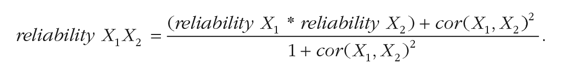
For example, if the true correlation between $X_1$ and $X_2$ is r = .20, $X_1$ has a reliability of 0.8, and $X_2$ has a reliability of 0.7, then the maximal observable correlation between $X_1$ and $X_2$ will be r = .15 ( $0.2\times \sqrt{0.7\times 0.8}$ ). In the case of an interaction, the reliability of the interaction term $X_1{X}_2$ is a function of the reliabilities of both $X_1$ and $X_2$ and the correlation between $X_1$ and $X_2$ (Busemeyer & Jones, 1983)

$$reliability{X}_1{X}_2=\frac{(reliability{X}_1*reliability{X}_2)+cor{(X_1,X_2)}^2}{1+cor{(X_1,X_2)}^2}.$$

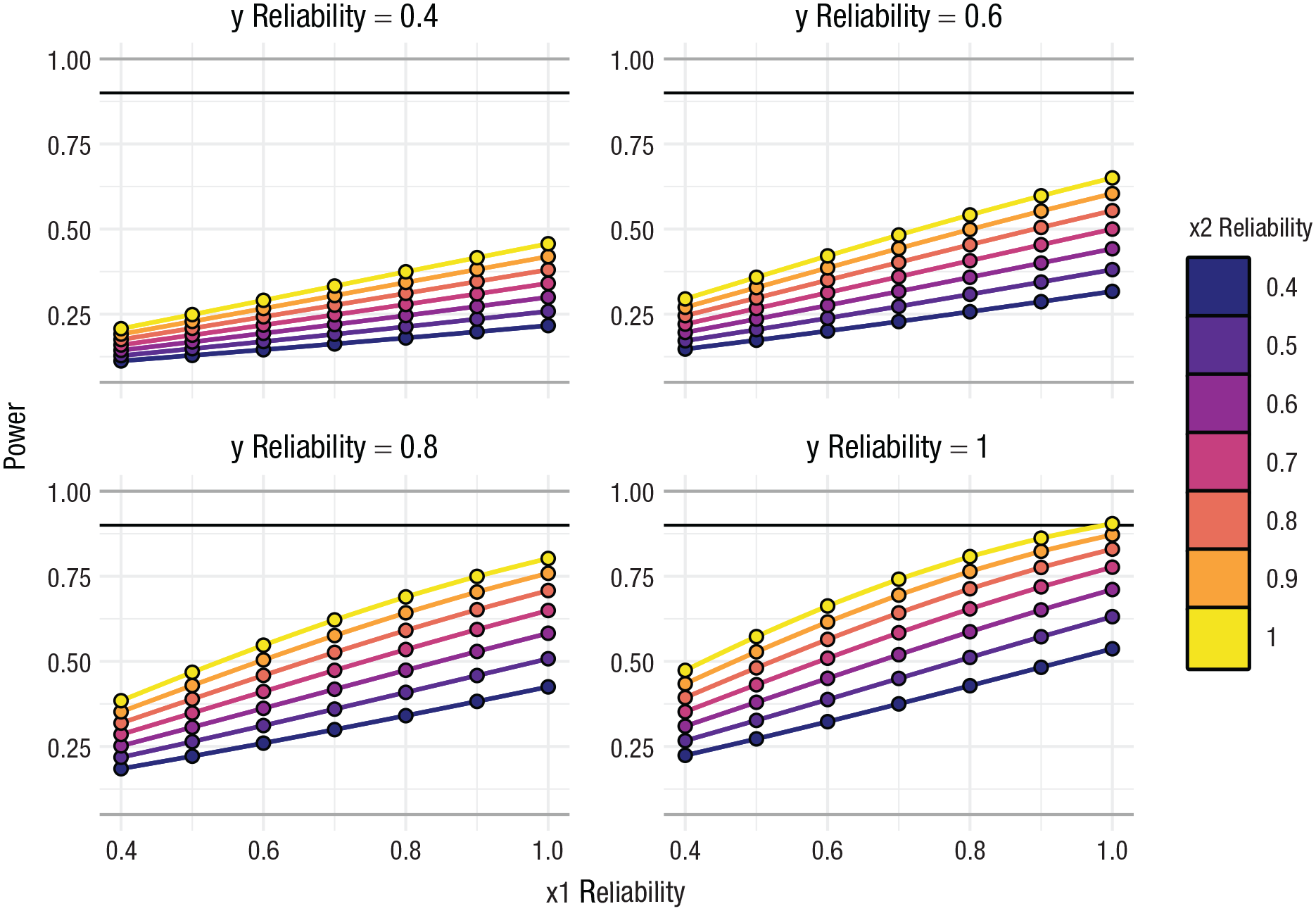
The lower bound of the reliability of $X_1{X}_2$ is simply the product of the reliabilities of $X_1$ and $X_2$ , although it will be greater than this (perhaps only marginally) if $X_1$ and $X_2$ are correlated. In the example above, the reliability of $X_1{X}_2$ would be .577 $\left(\frac{(0.7\times 0.8)+{0.2}^2}{1+{0.2}^2}\right)$ . Thus, the observable effect size for most interactions will be smaller (quite likely much smaller) than the true population effect size. We also note that reliability additionally affects power because it may attenuate other correlations in the analysis (between Y, $X_1,$ and $X_2$ ), thereby reducing the total variance explained by variables, which are independent of $X_1{X}_2$ (see “Main Effects and Their Correlation” above), further reducing the power of the analysis. Note that although the reliability of Y does not attenuate effect sizes, it does increase standard errors, thereby reducing power. Taking these effects together, you can see that any power analysis for interactions that does not account for reliability is liable to grossly overestimate power. Figure 6 shows an example of how the reliabilities of $X_1$ , $X_2,$ and Y compound to affect power.

Fig. 6.

Reliability. Example of the effect of reliability using the same effects as in Figure 1 (N = 940, the interaction effect is r = .09, the correlation between $X_1$ and Y is r = .51, the correlation between $X_2$ and Y is r = .22, and the correlation between $X_1$ and $X_2$ is r = .09). Reliability is controlled with the rel.x1, rel.x2, and rel.y flags and can also be adjusted in the online web apps. Although the analysis has 90% power when all variables have a reliability of 1.0, power decreases with less than perfect reliability. For example, with “good” reliability (all reliabilities are 0.8), the analysis has 60% power, and a sample size of 2,023 (more than double the size) would be required to achieve 90% power.

Binary and ordinal variables

It is frequently the case in the social and psychological sciences that not all variables are continuous. The power_interaction function allows users to specify that variables are binary (e.g., sex or group) or have multiple discrete levels (e.g., Likert scales). For example, Y can be a binary outcome, and analyses will be run as a logistic regression (Fig. 7a; note that the output of generate_interaction() is always z scored, but the test_interaction() and plot_interaction() functions detect that Y has two levels and convert it to a binary factor with levels 0 and 1 before analyses). Transforming a continuous variable to be discrete is well known to affect power in many cases because it attenuates correlations (Cohen, 1983). By setting the adjust.correlations flag to FALSE, users can evaluate the impact of a discrete transformation on power (Fig. 7b).

Fig. 7.

Binary and ordinal variables. (a) An example interaction when Y is a binary variable, run as a logistic regression. All other parameters are the same as in Figure 1a (the correlation between $X_1$ and Y is r = .51, the correlation between $X_2$ and Y is r = .22, the correlation between $X_1$ and $X_2$ is r = .09, and the interaction effect size is r = .09). (b) Y is continuous, and all parameters are the same as in Figure 7a. The sample size is 940. $X_1$ and $X_2$ are artificially discretized (thereby attenuating correlations) in the interaction_power_r2() function. The number of discrete values is set by the k.x1, k.x2, and k.y flags. If discretization is artificial (after the fact), set the adjust.correlations flag to FALSE (it is TRUE by default).

Selecting an Appropriate Effect Size

A power analysis cannot tell the user what interaction effect size is appropriate. However, prior work has found that interaction effects are commonly quite small. In a review of 261 articles in psychology journals that reported interaction effects, Aguinis et al. (2005) found a median effect of ${ƒ}^2$ = 0.002 (r ≈ .044). Recent work in personality science suggests that most replicable interaction effects are in fact smaller than this (Mdn r = .022; Vize et al., 2022). Likewise, recent work in human statistical genetics has found that although interactions are pervasive, they are largely orders of magnitude smaller than main effects (Zhu et al., 2022). These and related observations have led to prominent commentaries suggesting that researchers should plan on interaction effects that are at least a third of the size of main effects (i.e., an attenuated effect; Gelman, 2018) and theoretical work suggesting that most observable interactions are necessarily quite small (Tosh et al., 2021). Thus, if researchers are unsure what interaction effect to plan for or what shape to expect, we recommend planning for an attenuated interaction effect that is at least half the size of main effects.

We also remind the reader here that although there are many methods for determining the effects used in the power analysis, one should not draw these effects directly from an analysis that has already been performed (Gelman & Carlin, 2014; Zhang et al., 2019) unless one is planning a replication study. We recommend drawing effects from prior large studies and meta-analyses. In the absence of a published effect, we recommend conducting the power analysis at multiple reasonable values for the unknown parameter(s).

Conclusions

InteractionPoweR is a novel and useful addition to a researcher’s tool kit because it can easily compute power for statistical tests of interactions. It is currently the only package that allows users to set many of the parameters that affect power, including cross-sectional effect sizes, the correlation between variables, variable reliability, and variable distributions. Without considering all of these in tandem, one can arrive at an incorrect power estimate, possibly leading to either grossly underpowered or even overpowered (waste of resources) studies. Thus, the InteractionPoweR package can be a very helpful resource for researchers planning studies of interactions. Future work will seek to extend these power analyses to interaction models with covariates and mixed-effect models. Readers are recommended to see Table 2 for suggested further reading.

Table 2.

Selected References Recommended for Further Reading

Description	Citation
Power is strongly influenced by variance explained independent of the interaction term.	McClelland, G. H., & Judd, C. M. (1993). Statistical difficulties of detecting interactions and moderator effects. Psychological Bulletin, 114(2), 376–390. https://doi.org/10.1037/0033-2909.114.2.376
An interaction is not, in and of itself, evidence for a causal effect.	Rohrer, J. M., & Arslan, R. C. (2021). Precise answers to vague questions: Issues with interactions. Advances in Methods and Practices in Psychological Science, 4(2). https://doi.org/10.1177/25152459211007368
How to tell when interaction estimates will benefit from centering	Olvera Astivia, O. L., & Kroc, E. (2019). Centering in multiple regression does not always reduce multicollinearity: How to tell when your estimates will not benefit from centering. Educational and Psychological Measurement, 79(5), 813–826. https://doi.org/10.1177/0013164418817801
Issues surrounding omitted variable bias specific to interactions	Keller, M. C. (2014). Gene × environment interaction studies have not properly controlled for potential confounders: The problem and the (simple) solution. Biological Psychiatry, 75(1), 18–24. https://doi.org/10.1016/j.biopsych.2013.09.006
Estimated interaction effects are generally quite small.	Vize, C. E., Sharpe, B. M., Miller, J. D., Lynam, D. R., & Soto, C. J. (2022). Do the Big Five personality traits interact to predict life outcomes? Systematically testing the prevalence, nature, and effect size of trait-by-trait moderation. European Journal of Personality. Advance online publication. https://doi.org/10.1177/08902070221111857
Moving beyond simple slopes for the interpretation of interactions	Finsaas, M. C., & Goldstein, B. L. (2021). Do simple slopes follow-up tests lead us astray? Advancements in the visualization and reporting of interactions. Psychological Methods, 26(1), 38–60. https://doi.org/10.1037/met0000266
Study planning should consider more than just power.	Gelman, A., & Carlin, J. (2014). Beyond power calculations: Assessing Type S (Sign) and Type M (Magnitude) errors. Perspectives on Psychological Science, 9(6), 641–651. https://doi.org/10.1177/1745691614551642

Supplemental Material

sj-pdf-1-amp-10.1177_25152459231187531 – Supplemental material for Tutorial: Power Analyses for Interaction Effects in Cross-Sectional Regressions

Supplemental material, sj-pdf-1-amp-10.1177_25152459231187531 for Tutorial: Power Analyses for Interaction Effects in Cross-Sectional Regressions by David A. A. Baranger, Megan C. Finsaas, Brandon L. Goldstein, Colin E. Vize, Donald R. Lynam and Thomas M. Olino in Advances in Methods and Practices in Psychological Science

References

1.
AbersonC. L. (2019). Applied power analysis for the behavioral sciences (2nd ed.). Routledge, Taylor & Francis Group.
2.
AguinisH.BeatyJ. C.BoikR. J.PierceC. A. (2005). Effect size and power in assessing moderating effects of categorical variables using multiple regression: A 30-year review. Journal of Applied Psychology, 90(1), 94–107. https://doi.org/10.1037/0021-9010.90.1.94
3.
AikenL. S.WestS. G. (1991). Multiple regression: Testing and interpreting interactions. Sage.
4.
AltmejdA.DreberA.ForsellE.HuberJ.ImaiT.JohannessonM.KirchlerM.NaveG.CamererC. (2019). Predicting the replicability of social science lab experiments. PLOS ONE, 14(12), Article e0225826. https://doi.org/10.1371/journal.pone.0225826
5.
AndersonS. F.KelleyK. (2022). Sample size planning for replication studies: The devil is in the design. Psychological Methods. Advance online publication. https://doi.org/10.1037/met0000520
6.
BarangerD. A. A.FewL. R.SheinbeinD. H.AgrawalA.OltmannsT. F.KnodtA. R.BarchD. M.HaririA. R.BogdanR. (2020). Borderline personality traits are not correlated with brain structure in two large samples. Biological Psychiatry: Cognitive Neuroscience and Neuroimaging, 5(7), 669–677. https://doi.org/10.1016/j.bpsc.2020.02.006
7.
BeckE. D.JacksonJ. J. (2020). A mega-analysis of personality prediction: Robustness and boundary conditions. PsyArXiv. https://doi.org/10.31234/osf.io/7pg9b
BondyE.BarangerD. A. A.BalbonaJ.SputoK.PaulS. E.OltmannsT. F.BogdanR. (2021). Neuroticism and reward-related ventral striatum activity: Probing vulnerability to stress-related depression. Journal of Abnormal Psychology, 130(3), 223–235. https://doi.org/10.1037/abn0000618
10.
BrunnerJ.AustinP. C. (2009). Inflation of Type I error rate in multiple regression when independent variables are measured with error. Canadian Journal of Statistics, 37(1), 33–46. https://doi.org/10.1002/cjs.10004
11.
BusemeyerJ. R.JonesL. E. (1983). Analysis of multiplicative combination rules when the causal variables are measured with error. Psychological Bulletin, 93(3), 549–562. https://doi.org/10.1037/0033-2909.93.3.549
FaulF.ErdfelderE.LangA.-G.BuchnerA. (2007). G*Power 3: A flexible statistical power analysis program for the social, behavioral, and biomedical sciences. Behavior Research Methods, 39(2), 175–191. https://doi.org/10.3758/BF03193146
16.
FinsaasM. C.GoldsteinB. L. (2021). Do simple slopes follow-up tests lead us astray? Advancements in the visualization and reporting of interactions. Psychological Methods, 26(1), 38–60. https://doi.org/10.1037/met0000266
17.
FriedmanL.WallM. (2005). Graphical views of suppression and multicollinearity in multiple linear regression. The American Statistician, 59(2), 127–136.
GelmanA.CarlinJ. (2014). Beyond power calculations: Assessing Type S (Sign) and Type M (Magnitude) errors. Perspectives on Psychological Science, 9(6), 641–651. https://doi.org/10.1177/1745691614551642
20.
HainmuellerJ.MummoloJ.XuY. (2019). How much should we trust estimates from multiplicative interaction models? Simple tools to improve empirical practice. Political Analysis, 27(2), 163–192. https://doi.org/10.1017/pan.2018.46
21.
KellerM. C. (2014). Gene × environment interaction studies have not properly controlled for potential confounders: The problem and the (simple) solution. Biological Psychiatry, 75(1), 18–24. https://doi.org/10.1016/j.biopsych.2013.09.006
22.
KühbergerA.FritzA.ScherndlT. (2014). Publication bias in psychology: A diagnosis based on the correlation between effect size and sample size. PLOS ONE, 9(9), Article e105825. https://doi.org/10.1371/journal.pone.0105825
23.
LakensD.CaldwellA. R. (2021). Simulation-based power analysis for factorial analysis of variance designs. Advances in Methods and Practices in Psychological Science, 4(1). https://doi.org/10.1177/2515245920951503
McClellandG. H.JuddC. M. (1993). Statistical difficulties of detecting interactions and moderator effects. Psychological Bulletin, 114(2), 376–390. https://doi.org/10.1037/0033-2909.114.2.376
26.
Olvera AstiviaO. L.KrocE. (2019). Centering in multiple regression does not always reduce multicollinearity: How to tell when your estimates will not benefit from centering. Educational and Psychological Measurement, 79(5), 813–826. https://doi.org/10.1177/0013164418817801
27.
Open Science Collaboration. (2015). Estimating the reproducibility of psychological science. Science, 349(6251), Article aac4716. https://doi.org/10.1126/science.aac4716
28.
RevelleW.CondonD. M. (2019). Reliability from α to ω: A tutorial. Psychological Assessment, 31(12), 1395–1411. https://doi.org/10.1037/pas0000754
29.
RohrerJ. M.ArslanR. C. (2021). Precise answers to vague questions: Issues with interactions. Advances in Methods and Practices in Psychological Science, 4(2). https://doi.org/10.1177/25152459211007368
30.
RohrerJ. M.HünermundP.ArslanR. C.ElsonM. (2022). That’s a lot to process! Pitfalls of popular path models. Advances in Methods and Practices in Psychological Science, 5(2). https://doi.org/10.1177/25152459221095827
31.
ShermanR.PashlerH. (2019). Powerful moderator variables in behavioral science? Don’t bet on them (Version 3). PsyArXiv. https://doi.org/10.31234/osf.io/c65wm
32.
ShiehG. (2010). On the misconception of multicollinearity in detection of moderating effects: Multicollinearity is not always detrimental. Multivariate Behavioral Research, 45(3), 483–507. https://doi.org/10.1080/00273171.2010.483393
33.
SommetN.WeissmanD.CheutinN.ElliotA. J. (2022). How many participants do I need to test an interaction? Conducting an appropriate power analysis and achieving sufficient power to detect an interaction. OSF Preprints. https://doi.org/10.31219/osf.io/xhe3u
34.
SpearmanC. (1904). The proof and measurement of association between two things. The American Journal of Psychology, 15(1), 72–101. https://doi.org/10.2307/1412159
35.
ToshC.GreengardP.GoodrichB.GelmanA.VehtariA.HsuD. (2021). The piranha problem: Large effects swimming in a small pond. ArXiv. https://doi.org/10.48550/arXiv.2105.13445
36.
VizeC. E.SharpeB. M.MillerJ. D.LynamD. R.SotoC. J. (2022). Do the Big Five personality traits interact to predict life outcomes? Systematically testing the prevalence, nature, and effect size of trait-by-trait moderation. European Journal of Personality. Advance online publication. https://doi.org/10.1177/08902070221111857
WilmsR.MäthnerE.WinnenL.LanwehrR. (2021). Omitted variable bias: A threat to estimating causal relationships. Methods in Psychology, 5, Article 100075. https://doi.org/10.1016/j.metip.2021.100075
39.
ZhangY.HedoR.RiveraA.RullR.RichardsonS.TuX. M. (2019). Post hoc power analysis: Is it an informative and meaningful analysis?General Psychiatry, 32(4), Article e100069. https://doi.org/10.1136/gpsych-2019-100069
40.
ZhuC.MingM. J.ColeJ. M.KirkpatrickM.HarpakA. (2022). Amplification is the primary mode of gene-by-sex interaction in complex human traits. bioRxiv. https://doi.org/10.1101/2022.05.06.490973
Supplementary Material
Please find the following supplemental material available below.
For Open Access articles published under a Creative Commons License, all supplemental material carries the same license as the article it is associated with.
For non-Open Access articles published, all supplemental material carries a non-exclusive license, and permission requests for re-use of supplemental material or any part of supplemental material shall be sent directly to the copyright owner as specified in the copyright notice associated with the article.